A Cost Metric for Team Efficiency

We use a Riemannian metric as a cost metric when it comes to the optimal decisions that should be made in a multi-agent/Team scenario. The two parameters of interest to us are Team skill and Team interdependence, which are modeled as Wiener process drift and the inverse of Wiener process diffusion, respectively. The underlying mathematics is presented, along with some approximating rules of thumb. It is noteworthy that the mathematics points to, what seems at first, counter-intuitive paradigms for Team performance. However, in reality the mathematics shows a subtle interplay between the factors affecting Team performance.

1 Introduction

We are concerned here with how a multi-agent System (MAS) [2], or Team, reaches the successful conclusion of a task. In Team science, an important parameter for success is interdependence [1, 9, 10, 12]. The Team may be human, machine, or a hybrid. However, our mathematical assumptions implicitly assume that the Team is very machine-like in its behavior and discounts the vagaries of human psychology, e.g., [5]. We address this further at the conclusion of this article.

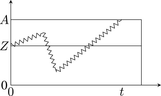
In [13] it was shown how to model Team behavior as (1-dimensional) Brownian motion [4] (starting at a point Z on the line). In particular, we proposed using Brownian motion $\mathcal{B}(t)$ with (high) drift μ, for (high) Team skill and (low) diffusion σ, for (high) interdependence, arbitrarily starting at a point Z, 0 ≤ Z ≤ A. We consider that the Team has succeeded if it reaches point A before 0, and the Team has failed if it reaches 0 before A.

The drift, as mentioned, models Team skill. By way of motivation (using humans), imagine we have a restaurant kitchen crew (building on the restaurant Team given in [11]). We would like all the Team members to have the most skill possible; this would go into the calculation of the drift μ. High skill mapping to high μ. We would also like the Team to work together, hence we desire a high interdependence. Interdependence is the inverse of the diffusion, thus a Team with high interdependence has low diffusion σ, and a Team with each Team member acting independently of the other has high diffusion σ. This leads to the question of which is better—high drift μ, or low diffusion σ? Again, let us go back to our kitchen crew example. If everyone in the kitchen is skilled, but working independently of the others, the result will be a disaster. The dessert will be served before the main course, wine will be served after dessert, etc. Thus, skill alone does not lead to optimal success. On the other hand, consider a kitchen crew with no skill, but working together hand in glove. The results here are also less than optimal—very bad food served in an efficient manner. What is needed is a combination of both factors for optimal Team success, and that is what our idealized mathematics show.

Definition 1. We say that a stochastic process ${\mathcal{W}}_t,t\ge 0$ is a Wiener process [8] if

• ${\mathcal{W}}_0=0$.

• With probability 1, the function $t{\to \mathcal{W}}_t$ is continuous in t.

• The stochastic process $\left\{{\mathcal{W}}_t\right\},t\ge 0$, has stationary, independent increments.

• The increment, ${\mathcal{W}}_{t+s}{-\mathcal{W}}_s$, has the distribution of the standard normal random variable, N (0, t) (this latter part of the definition tells us that ${\mathcal{W}}_t$ has the distribution of N (0, t)).

Definition 2. From [13, 15, 17, 18], we say that $\mathcal{B}(t)$ is Brownian motion with drift μ and diffusion σ, that starts at Z, 0 ≤ Z ≤ A, if

$\mathcal{B}\left(t\right)=\mu t+\sigma \mathcal{W}\left(t\right)+Z.(1)$

Let $P_Z(\partial \stackrel{̄}{}=0)$ be the probability that $\mathcal{B}(t)$ hits the bottom boundary first (Team failure), then $P_Z(\partial \stackrel{̄}{}=A)=1-P_Z(\partial \stackrel{̄}{}=0)$ is the probability that it hits the top boundary first (Team success). Figure 1 is an example of such a sample path. These probabilities are derived from stopping probabilities ([3]), and we use L’Hôpital’s rule for μ = 0.

$P_Z\left(\partial \stackrel{̄}{}=0\right)=\left\{\begin{array}{cc}\frac{e^{-\frac{2A\mu }{{\sigma }^2}}-e^{-\frac{2Z\mu }{{\sigma }^2}}}{e^{-\frac{2A\mu }{{\sigma }^2}}-1},\hfill & \text{if\hspace{0.17em}}\mu \ne 0\hfill \\ 1-\frac{Z}{A},\hfill & \mu =0\hfill \end{array}\right.(2)$

and

$P_Z\left(\partial \stackrel{̄}{}=A\right)=\left\{\begin{array}{cc}\frac{e^{-\frac{2Z\mu }{{\sigma }^2}}-1}{e^{-\frac{2A\mu }{{\sigma }^2}}-1},\hfill & \text{if\hspace{0.17em}}\mu \ne 0\hfill \\ \frac{Z}{A},\hfill & \mu =0.\hfill \end{array}\right.(3)$

FIGURE 1

FIGURE 1. Brownian motion, $\mathcal{B}(t)$, starting at Z and with absorbing boundaries at A (top) and 0 (bottom).

For now, we will concentrate on Equation 3. Keep in mind that as σ → 0, then $P_Z(\partial \stackrel{̄}{}=A)\to 1$, if μ > 0, and that $P_Z(\partial \stackrel{̄}{}=A)\to 0$, if μ < 0 (of course, if Z > A, this would not hold).

For Z = 0, we have that $P_Z(\partial \stackrel{̄}{}=A)=0$ since 0 is an absorbing boundary—that is, if we start at 0 we are done. Also, for Z = A, we have that $P_Z(\partial \stackrel{̄}{}=A)=1$, which also makes sense—if we start at A, we never leave A.

Now say that we need to make an assessment—is it better to modify the drift μ or modify the diffusion σ to increase $P_Z(\partial \stackrel{̄}{}=A)$? Also, what is the cost of this modification, and how do we measure the cost?

2 First Steps

We start by defining our manifold B and its Riemannian structure.¹

2.1 Our Manifold B

We would like to know the costs of changing $P_Z(\partial \stackrel{̄}{}=A)$ as we vary μ and σ. We consider $\mathcal{B}(t)$ in terms of its two parameters, μ and σ.

With this in mind, we define a 2-dimensional Riemannian manifold B, homeomorphic to $\mathbb{R}\times {\mathbb{R}}^{+}$, and with a global μ, σ chart. We give B the Riemannian metric

${ds}^2=d\mu \otimes d\mu +\frac{1}{{\sigma }^2}d\sigma \otimes d\sigma .(4)$

This metric captures the fact that for σ fixed, the difference in μ is simply the standard L₁ distance between them, and that it is independent of the diffusion value. However, the diffusion is also independent of the drift value, but as we attempt to make the diffusion (standard deviation) smaller, it costs more and more, until we approach ∞ at the Dirac distribution.

Note 1—We have chosen to give an infinitesimal distance between points (μ, σ) and (μ + dμ, σ + dσ) and then extend it to a global distance. The Riemannian metric ds² captures the fact that changes in μ are Euclidean straight-line distance, whereas changes in σ are based on the inverse of the variance. This concept aligns with how normal distributions differ. We further note that this result is also similar to the Fisher information of the normal distribution (a normalized Poincaré upper-half-plane). What is important about our Riemannian metric is that only the dσ² is modified from the standard Euclidean metric. Again, this emphasizes the fact that changing the mean of the normal distribution is strictly Euclidean, whereas if we attempt to lower the variance, it requires much more “power,” and in the limit approaches infinite power. This approach agrees with our thinking that total interdependence (exactly the opposite of independent behavior) has a diffusion of 0, where as totally uncorrelated behavior has infinite diffusion [13, 6.4.2].—

Thus, B has the first fundamental form

$\left[g_{ij}\right]=\left(\begin{array}{cc}\hfill E\hfill & \hfill F\hfill \\ \hfill F\hfill & \hfill G\hfill \end{array}\right)=\left(\begin{array}{cc}\hfill 1\hfill & \hfill 0\hfill \\ \hfill 0\hfill & \hfill \frac{1}{{\sigma }^2}\hfill \end{array}\right),\text{\hspace{0.17em}where\hspace{0.17em}}i,j\text{are\hspace{0.17em}indexed\hspace{0.17em}independently\hspace{0.17em}over\hspace{0.17em}}\mu ,v.(5)$

Assume we are at p ∈ B, where p = (p_μ, p_σ), and with tangent vectors $\widehat{U}=u_1\widehat{\frac{\partial }{\partial \mu }}+u_2\widehat{\frac{\partial }{\partial \sigma }}$, $\widehat{W}=w_1\widehat{\frac{\partial }{\partial \mu }}+w_2\widehat{\frac{\partial }{\partial \sigma }}$ at p, where $\widehat{\frac{\partial }{\partial \mu }},\widehat{\frac{\partial }{\partial \sigma }}$ are the canonical basis for the tangent space at p.

The inner product between them is

$⟨\widehat{U},\widehat{W}⟩≔u_1{w}_1+\frac{1}{{\left(p_{\sigma }\right)}^2}{u}_2{w}_2.$

The norm of a vector $\widehat{W}$ is

$\Vert \widehat{W}\Vert ≔\sqrt{⟨\widehat{W},\widehat{W}⟩}.$

Say c(t) is a smooth curve in B, c: (a, b) → B, then there is the velocity vector field (on the curve) denoted as $\dot{c}(t)$. This velocity vector field assigns to each point c(t′) on the curve c(t) the velocity vector (which is also a tangent vector of M) of the curve at c(t′) expressed as $\dot{c}(t^{\prime })$ (keep in mind that this is multi-dimensional).

That is, c(t) = (c_μ(t), c_σ(t)), and $\dot{c}(t)={\dot{c}}_{\mu }(t)\widehat{\frac{\partial }{\partial \mu }}+{\dot{c}}_{\sigma }(t)\widehat{\frac{\partial }{\partial \sigma }}$ (where the raised dot symbol is the usual differentiation with respect to t, and $\widehat{\frac{\partial }{\partial \mu }},\widehat{\frac{\partial }{\partial \sigma }}$ are understood to be the canonical tangent space basis vectors at the point c(t) ∈ M). To simplify notation, we can express this as $\dot{c}(t)=⟨{\dot{c}}_{\mu }(t),{\dot{c}}_{\sigma }(t)⟩$.

We define the length of c(t), denoted as L(c), as

$L\left(c\right)≔{\int }_a^b\Vert \dot{c}\left(\tau \right)\Vert d\tau ={\int }_a^b\sqrt{{\left[{\dot{c}}_{\mu }\left(\tau \right)\right]}^2+\frac{{\left[{\dot{c}}_{\sigma }\left(\tau \right)\right]}^2}{{\left[c_{\sigma }\left(\tau \right)\right]}^2}}d\tau .(6)$

Given two points, p, q ∈ B, and c(t), any smooth curve between them (this can be relaxed to include piece-wise smooth, but not of class C^∞), we define the distance between them as

$d\left(p,q\right)≔\inf L\left(c\right).(7)$

2.2 Team Geometry

Our metric is modeled on the hyperbolic metric in the Poincaré half-plane model. An important difference is that E does not depend on the σ value. The change in drift is independent of the diffusion value which we feel is the correct way to model Team action. Furthermore, the μ distance is linear with respect to μ. This choice assumes that only the change of Team skill matters, not the values it ranges between. However, the change in diffusion, which is independent of drift, does depend on the different diffusion (interdependence values) that the Team is choosing between. This approach makes sense in terms of a normal distribution. Going from a normal distribution N (μ, 10) to N (μ, 9) requires much less change in the distribution itself than going from N (μ, 1) to N (μ, 0.9), and again going from N (μ, 0.5) to N (μ, 0.45).

We see in Figure 2 that as σ → 0⁺, the difference in the normal plots is more severe. This behavior is in contrast to changing μ, which has the effect of shifting the graph to the left or right, but not changing its shape. We use a Riemannian manifold because it gives us the means to modify the metric for other models of Team behavior. This approach is accomplished by adjusting the g_ij in Equation 5.

FIGURE 2

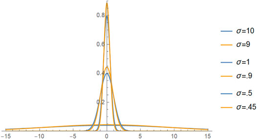
FIGURE 2. N (0, σ²) for three groups. g The bottom pair is σ = 10, 9; the middle pair is σ = 1, 0.9; and the top two, which are the most different are σ = 0.5, 0.45.

2.3 Curvature and Geodesics

We start by considering the Gaussian (sectional) curvature K of B as a function of the first fundamental form.

First, using Equation 5, we consider the easily obtainable matrices (the sub-index indicates the partial differentiation with respect to that index) for B.

$\left(\begin{array}{cc}\hfill E_{\mu }\hfill & \hfill F_{\mu }\hfill \\ \hfill F_{\mu }\hfill & \hfill G_{\mu }\hfill \end{array}\right)=\left(\begin{array}{cc}\hfill 0\hfill & \hfill 0\hfill \\ \hfill 0\hfill & \hfill 0\hfill \end{array}\right)\text{\hspace{0.17em}and\hspace{0.17em}}\left(\begin{array}{cc}\hfill E_{\sigma }\hfill & \hfill F_{\sigma }\hfill \\ \hfill F_{\sigma }\hfill & \hfill G_{\sigma }\hfill \end{array}\right)=\left(\begin{array}{cc}\hfill 0\hfill & \hfill 0\hfill \\ \hfill 0\hfill & \hfill \frac{-2}{{\sigma }^3}\hfill \end{array}\right).(8)$

From [14, Eq. (9.22), Eq. (9.33)] we use the Brioschi formula for a Riemannian 2-manifold in general with generic parameters μ, v, which, for arbitrary E and G, and when F = 0 [14, Eq. 9.25], becomes

$\begin{array}{ccc}\hfill K& =\hfill & \frac{-1}{\sqrt{EG}}\left\{\frac{\partial }{\partial \mu }\left(\frac{1}{\sqrt{E}}\frac{\partial \sqrt{G}}{\partial \mu }\right)+\frac{\partial }{\partial \sigma }\left(\frac{1}{\sqrt{G}}\frac{\partial \sqrt{E}}{\partial \mu }\right)\right\}\hfill \end{array}(9)$

$\begin{array}{ccc}\hfill & =\hfill & \frac{-1}{2\sqrt{EG}}\left\{\frac{\partial }{\partial \mu }\left(\frac{G_{\mu }}{\sqrt{EG}}\right)+\frac{\partial }{\partial \sigma }\left(\frac{E_{\sigma }}{\sqrt{EG}}\right)\right\}.\hfill \end{array}(10)$

For B, G_μ = 0 and E_σ = 0, we find that K = 0.

Now we move on to the geodesics of B. First we have to find the Christoffel (tensor) symbols (symmetric in the lower indicies). We define these on a local patch of a Riemannian 2-manifold, M, in general with generic parameters μ, σ.

$\begin{array}{ccc}\hfill {\mathrm{\Gamma }}_{\mu \mu }^{\mu }& =\hfill & \frac{G{E}_u+F{E}_{\sigma }-2F{F}_u}{2\left(EG-F^2\right)}\hfill \end{array}(11)$

$\begin{array}{ccc}\hfill {\mathrm{\Gamma }}_{\mu \sigma }^{\mu }& =\hfill & \frac{G{E}_{\sigma }-F{G}_u}{2\left(EG-F^2\right)}\hfill \end{array}(12)$

$\begin{array}{ccc}\hfill {\mathrm{\Gamma }}_{\sigma \sigma }^{\mu }& =\hfill & \frac{-F{G}_{\sigma }-G{G}_u+2G{F}_{\sigma }}{2\left(EG-F^2\right)}\hfill \end{array}(13)$

$\begin{array}{ccc}\hfill {\mathrm{\Gamma }}_{\mu \mu }^{\sigma }& =\hfill & \frac{-F{E}_u-E{E}_{\sigma }+2E{F}_u}{2\left(EG-F^2\right)}\hfill \end{array}(14)$

$\begin{array}{ccc}\hfill {\mathrm{\Gamma }}_{\mu \sigma }^{\sigma }& =\hfill & \frac{E{G}_u-F{E}_{\sigma }}{2\left(EG-F^2\right)}\hfill \end{array}(15)$

$\begin{array}{ccc}\hfill {\mathrm{\Gamma }}_{\sigma \sigma }^{\sigma }& =\hfill & \frac{E{G}_{\sigma }+F{G}_u-2F{F}_{\sigma }}{2\left(EG-F^2\right)}.\hfill \end{array}(16)$

Thus, for our manifold B, we have that all of the Christoffel symbols are 0, except for ${\mathrm{\Gamma }}_{\sigma \sigma }^{\sigma }=\frac{-1}{\sigma }.$

Definition 3. For t ∈ (0, 1), a smooth curve c(t) = (c₁(t), c₂(t)), $\dot{c}(t)=({\dot{c}}_1(t),{\dot{c}}_2(t))$ in a Riemannian manifold with ∇ being the Levi-Civita connection [20] is a geodesic if

${\nabla }_{\dot{c}\left(t\right)}\dot{c}\left(t\right)=0.(17)$

In general, one does not need to restrict t to the unit interval, but we have done this as a convenience. In general, geodesics are unique up to an affine parametrization; without loss of generality, we have fixed this by setting the t interval to [0, 1]. Note that by the existence and uniqueness theorem for ordinary differential equations (ODEs), we can find a unique geodesic if we also include the vector values at c (0) and c′(0). (It turns out for B that this follows directly.)

We do not want to get into too many of the details of the ∇ operator above. It is covariant differentiation, which is the directional derivative of the vector field $\dot{c}(t)$ in the direction $\dot{c}(t)$ with adjustments for curvature K. Details can be readily found in the literature (e.g. [14]). Since the one local coordinate system (patch) we have given for B suffices, the geodesic equation reduces to

$\begin{array}{ccc}\hfill {\ddot{c}}_{\mu }\left(t\right)+\sum _{i,j\in \left\{\mu ,\sigma \right\}}{\mathrm{\Gamma }}_{ij}^{\mu }{\dot{c}}_i\left(t\right){\dot{c}}_j\left(t\right)=0,\text{\hspace{0.17em}and}& \hfill & \hfill \end{array}(18)$

$\begin{array}{ccc}\hfill {\ddot{c}}_{\sigma }\left(t\right)+\sum _{i,j\in \left\{\mu ,\sigma \right\}}{\mathrm{\Gamma }}_{ij}^{\sigma }{\dot{c}}_i\left(t\right){\dot{c}}_j\left(t\right)=0,& \hfill & \hfill \end{array}(19)$

which, using the above values of the Christoffel symbols, simplifies to

$\begin{array}{ccc}\hfill {\ddot{c}}_{\mu }\left(t\right)=0,\text{\hspace{0.17em}and}& \hfill & \hfill \end{array}(20)$

$\begin{array}{ccc}\hfill {\ddot{c}}_{\sigma }\left(t\right)-\frac{{\left({\dot{c}}_{\sigma }\right)}^2}{c_{\sigma }\left(t\right)}=0.& \hfill & \hfill \end{array}(21)$

Trivially, we find that

$c_{\mu }\left(t\right)=at+b.$

To obtain c_σ(t), we need to solve a non-linear second order ODE, so we simplify notation and use the auxiliary variable $w={\dot{c}}_{\sigma }$, which gives ${\ddot{c}}_{\sigma }=\frac{dw}{d{c}_{\sigma }}{\dot{c}}_2=\frac{dw}{d{c}_{\sigma }}w$. Now we perform the usual trickery, but check our answer at the end.

$\begin{array}{ccc}\hfill {\ddot{c}}_{\sigma }& =\hfill & \frac{{\left({\dot{c}}_{\sigma }\right)}^2}{c_{\sigma }}\hfill \\ \hfill \frac{dw}{d{c}_{\sigma }}w& =\hfill & \frac{w^2}{c_{\sigma }}\hfill \\ \hfill \frac{dw}{w}& =\hfill & \frac{d{c}_{\sigma }}{c_{\sigma }}\hfill \\ \hfill w& =\hfill & \beta c_{\sigma }\hfill \\ \hfill {\dot{c}}_{\sigma }& =\hfill & \beta c_{\sigma }\hfill \\ \hfill c_{\sigma }\left(t\right)& =\hfill & \alpha e^{\beta t}.\hfill \end{array}$

which when we check does solve Eq. 21 for c_σ(t) in its most general form. Thus,

$c\left(t\right)=\left(at+b,\alpha e^{\beta t}\right).(22)$

Theorem 1. The constants a, b, α, β uniquely fix the geodesic.

Proof. Say there are two geodesics $c,\bar{c}:[\mathrm{0,1}]\to \mathbf{B}$ such that

$c\left(t\right)=\left(at+b,\alpha e^{\beta t}\right),\text{and}$

$\bar{c}\left(t\right)=\left(\bar{a}t+\bar{b},\bar{\alpha }{e}^{\bar{\beta }t}\right).$

Assume they are the same geodesic; then by evaluating the geodesic at t = 0, we have that

$b=\bar{b},\alpha =\bar{\alpha }.$

Now using the above and evaluating the geodesics at t = 1, we have that

$a=\bar{a},\beta =\bar{\beta }.$

□

So all we have to do now is to determine the four constants in the geodesic curve to uniquely specify it. As noted above, if we specify c(0) = (μ₀, σ₀) and $\dot{c}(0)=(\aleph ,\beth )$, then simple calculations show that we uniquely fix the geodesic as

$c\left(t\right)=\left(\aleph t+{\mu }_0,v_0{e}^{\frac{\beth }{{\sigma }_0}t}\right).(23)$

However, we are interested in the boundary value problem to see if knowing c(0), c′(0) also gives us a unique solution. In general, for geodesics on an arbitrary Riemannian manifold, this result need not be true. By way of example, consider the geodesics (where the locus is a great circle) on S². Given c(0), c(1), there are infinitely many geodesics that satisfy the conditions (they just keep wrapping around). What is different in our situation, however, is that the geodesics never go back on themselves (this is seen by looking at the form of c(t)). If we have that c(0) = (μ₀, σ₀) and c(1) = (μ₁, σ₁), then simple calculations show that these boundary conditions uniquely fix the geodesic as

$c\left(t\right)=\left({\mu }_0+\left({\mu }_1-{\mu }_0\right)t,{\sigma }_0{e}^{t\ln \left(\frac{{\sigma }_1}{{\sigma }_0}\right)}\right)=\left({\mu }_0+\left({\mu }_1-{\mu }_0\right)t,{\sigma }_0{\left(\frac{{\sigma }_1}{{\sigma }_0}\right)}^t\right).(24)$

Thus, for the geodesics c: [0, 1] → B, we find that a solution exists and, given c(0) and c(1), that the geodesic is uniquely expressed as in Equation 24.

Equations 6 and 7 tell us how to obtain a topology based on the metric distance. This topology makes B homeomorphic to the upper half-plane with its standard topology. (Note though that B is not isometric to the upper half-plane with the standard Euclidean metric.) Since the latter space is complete, so is B. By the Hopf-Rinow theorem [20], given an initial point p = (x₀, y₀), and a final point q = (x₁, y₁), there exists a geodesic c(t) between them such that c (0) = p, c (1) = q and L(c) = d (p, q). Given Equation 24, we have shown how to uniquely construct such a geodesic; therefore, the geodesic from Equation 24 has the property that its length is the distance between the points.

The message from this result is that, given two points p, q on B, if we find the geodesic between them (remember we only use as a domain [0, 1]), then the length of that geodesic is the distance between them. This result is similar to what occurs in the Poincaré upper half-plane. We also note that this result would not work on S² because the boundary values do not uniquely determine the geodesic—as discussed above, the geodesics on S² can wrap around themselves, which does not happen on B or the Poincaré upper half-plane. Therefore, this leaves us with the following corollary to the above theorem.

Corollary 1.1. Given two points in p = (μ₀, v₀) ∈ B, and q = (μ₁, σ₁) ∈ B, there is a unique geodesic c: [0, 1] → B between them such that c(0) = p, c(1) = q. Furthermore, c(t) is length minimizing, that is, L(c) = d (p, q). The geodesic is as given in Equation 24.

Now let us examine the length of our geodesic c(t) between p = (μ₀, σ₀) and q = (μ₁, σ₁). By Equation 6, we have that. $L(c)={\int }_0^1\sqrt{{({\mu }_1-{\mu }_0)}^2+{\left[\ln \left(\frac{{\sigma }_1}{{\sigma }_0}\right)\right]}^2}d\tau \text{,\hspace{0.17em}thus,\hspace{0.17em}}$

Corollary 1.2. Given two points in p = (μ₀, σ₀) ∈ B, q = (μ₁, σ₁) ∈ B, the length of the unique geodesic c(t) between them is

$\sqrt{{\left({\mu }_1-{\mu }_0\right)}^2+{\left[\ln \left(\frac{{\sigma }_1}{{\sigma }_0}\right)\right]}^2}.(25)$

Let us see what some of these geodesics look like (their traces).

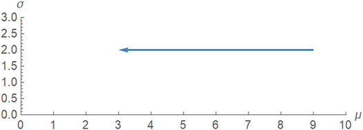
Example 1: Let us examine the case where σ is held constant between two points. Let p = (μ₁, σ), q = (μ₂, σ). The geodesic between them is

$c\left(t\right)=\left({\mu }_0+\left({\mu }_1-{\mu }_0\right)t,\sigma \right).$

We illustrate this result with p = (9, 2), q = (3, 2) in Figure 3. When v is fixed, we are in a standard Euclidean metric, the length of the geodesic is its distance, and it follows from Eqs 6, 7 that d (p, q) = |μ₁ − μ₀|,

FIGURE 3

FIGURE 3. Geodesic starting at p = (9, 2) and ending at q = (3, 2).

The result is a horizontal straight line of length six. When v is fixed, our geometry is standard Euclidean geometry. Example 2: Let us now look at the opposite situation, when we hold μ fixed and vary σ.

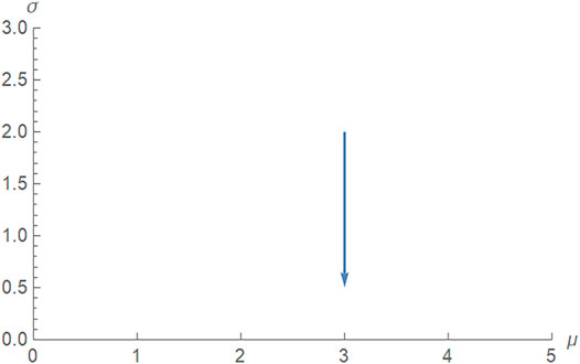
The trace of this geodesic, shown in Figure 4, is simply a vertical line, however, its length is not its Euclidean length of 2—0.5 = 1.5, rather its length is $\left|\ln (.5/2)\right|=1.39$. The geometry here is far from Euclidean. But now let us consider the geodesic starting at p = (3, 0.2) and ending at q = (3, 0.05). Again, its length is not the Euclidean length of 0.15; rather, its length is $\left|\ln (.05/.2)\right|=1.39$, the same as the first part of this example. Let us summarize these two examples. For B, the length of a geodesic connecting two points with fixed σ is simply their Euclidean distance. However, the length of a geodesic in B connecting two points with the same μ only depends on their ratio, the distance being the absolute value of the natural log of the ratio.

FIGURE 4

FIGURE 4. Geodesic starting at p = (3, 2) and ending at q = (3, 0.5).

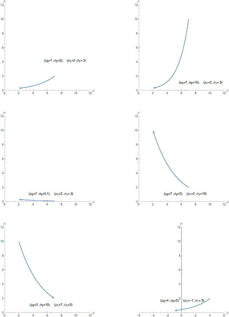
Let us look at the general geodesics a bit more. In Figure 5, we see paths of the geodesics that start at (μ₀, σ₀) and end at (μ₁, σ₁). These representative samples, along with Figures 3, 4, show the general shape of the geodesics.

FIGURE 5

FIGURE 5. Various geodesics.

An interesting question becomes: Given a point (μ₀, σ₀), what is the locus of points (μ, σ) distance D from this point? From Equation 25, we easily have that

$\sigma ={\sigma }_0{e}^{\pm \sqrt{D^2-{\left(\mu -{\mu }_0\right)}^2}}.(26)$

From this result, we see that μ ∈ [μ₀ − D, μ₀ + D] and σ ∈ [σ₀e^−D, σ₀e^D].

We plot in Figure 6 the locus of points for σ as a 2-valued “function” of μ, with distance 2 from the point (1.5, 3) and when Z=.6 (recall that we have normalized A to 1).

FIGURE 6

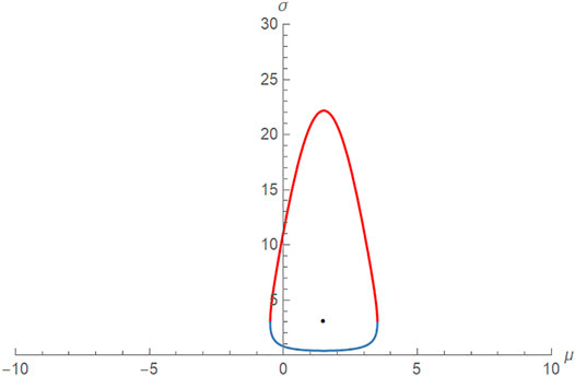
FIGURE 6. Geodesic locus: Points at a distance 2 from (1.5, 3) with A = 1, Z =0.6. This is our metric “circle.”

Let us go back to Eq. 3 and see how $P_{.6}(\partial \stackrel{̄}{}=1)$ varies as we look at all of the points at a set distance from (μ₀, σ₁).

We start by summarizing some of the results from [16, Sec 6.2.2] that discuss how $P_Z(\partial \stackrel{̄}{}=A)$ behaves.

• $P_Z(\partial \stackrel{̄}{}=A)$ is an increasing function of μ.

• For μ > 0, $P_Z(\partial \stackrel{̄}{}=A)$ is a decreasing function of σ.

• For μ < 0, $P_Z(\partial \stackrel{̄}{}=A)$ is an increasing function of σ.

Since the center of our 2-ball is (1.5, 3), let us examine the two points with extreme μ values of -0.5 and 3.5. We find that

$P_{.6}\left(\partial \stackrel{̄}{}=1\right){|}_{\left(-.\mathrm{5,3}\right)}=.587<P_{.6}\left(\partial \stackrel{̄}{}=1\right){|}_{\left(1.5,3\right)}=.639<P_{.6}\left(\partial \stackrel{̄}{}=1\right){|}_{\left(3.5,3\right)}=.690,$

and

$P_{.6}\left(\partial \stackrel{̄}{}=1\right){|}_{\left(3.5,.406\right)}=.999>P_{.6}\left(\partial \stackrel{̄}{}=1\right){|}_{\left(1.5,3\right)}=.639>P_{.6}\left(\partial \stackrel{̄}{}=1\right){|}_{\left(3.5,22.17\right)}=.601.$

Keep in mind that for μ fixed at 3.5, as σ grows, the boundary probability approaches 0.6 = Z/A = 0.6/1. This results in the values at the four “corners” of the metric-circle. One might think that the south pole is the highest probability. Let us plot $P_Z(\partial \stackrel{̄}{}=A)=1$ as a 2-valued function of μ. That is, we plot $P_Z(\partial \stackrel{̄}{}=A)=1$ as a function of μ with $\sigma ={\sigma }_0{e}^{\sqrt{D^2-{(\mu -{\mu }_0)}^2}}$ (which corresponds to the top red semi-circle) and $\sigma ={\sigma }_0{e}^{-\sqrt{D^2-{(\mu -{\mu }_0)}^2}}$ (which corresponds to the bottom blue semi-circle). The range of μ is μ ∈ [μ₀ − D, μ₀ + D]. The point $(\mu ,e^{\sqrt{D^2-{(\mu -{\mu }_0)}^2}})$ has a lesser probability than $(\mu ,e^{-\sqrt{D^2-{(\mu -{\mu }_0)}^2}})$, since for μ fixed, the smaller σ becomes, the greater the probability when μ is positive.

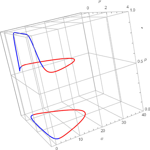
Please note when comparing Figures 6, 7 that the blue and red regions have shifted.

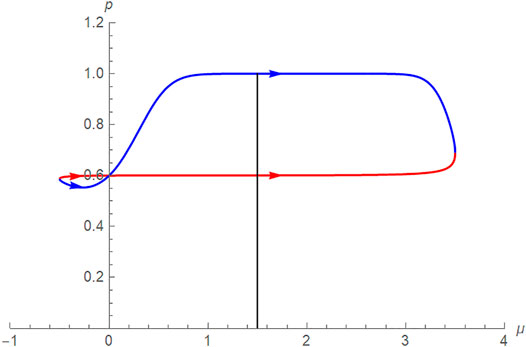
FIGURE 7

FIGURE 7. $P_{.6}(\partial \stackrel{̄}{}=1)$ of point distance 2 from (μ, σ) = (1.5, 3) as μ increases (indicated by arrow direction) from −0.5 to 3.5. We see that for negative drift, the probabilities have an inverse behavior.

From Figure 7, one might infer that the maximum probability occurs at the bottom corner (μ, σ) = (1.5, 0.406). Further numerical analysis shows that this is not true; the actual maximum occurs closer to when μ = 2 (with the corresponding σ > 0.406). Let us use a different example to show this result better, as in Figure 8. Here, it is much more obvious that the maximum probability does not occur at the south pole of the metric circle.

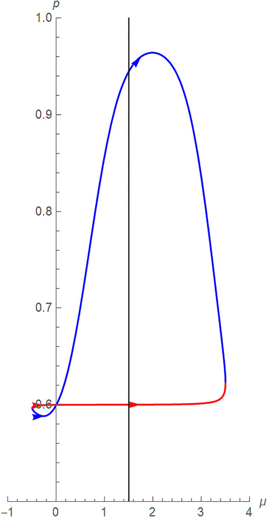
FIGURE 8

FIGURE 8. $P_{.6}(\partial \stackrel{̄}{}=1)$ of points distance 2 from (μ, σ) = (1.5, 6) as μ increases (indicated by the arrow’s direction) from −0.5 to 3.5.

We also see that the minimum probability does not occur for the smallest μ; rather, it too is a combination of a small μ, but with a larger σ.

In Figure 9, we have combined the plots from Figures 6, 7. That is, Figure 6, which is a plot of a 2-valued function of σ against μ, is sketched in (μ, σ, 0) space. In Figure 7, since σ is now a 2-valued function of μ, we see that the probability $P_{.6}(\partial \stackrel{̄}{}=1)$ (of points distance 2 from the center (1.5, 3)) is a 2-valued function of μ and lives naturally in (μ, σ, p) space. In other words, the points on the top of a point of distance 2 is on the top plot. The red curves correspond to $\sigma =3e^{\sqrt{2^2-{(\mu -1.5)}^2}}$, and the blue curves correspond to $\sigma =3e^{-\sqrt{2^2-{(\mu -1.5)}^2}}$. We see that the red probability hovers around 0.6, whereas the blue approaches, very closely in fact, to a probability of 1.

FIGURE 9

FIGURE 9. Combo.

3 Surface Geometry

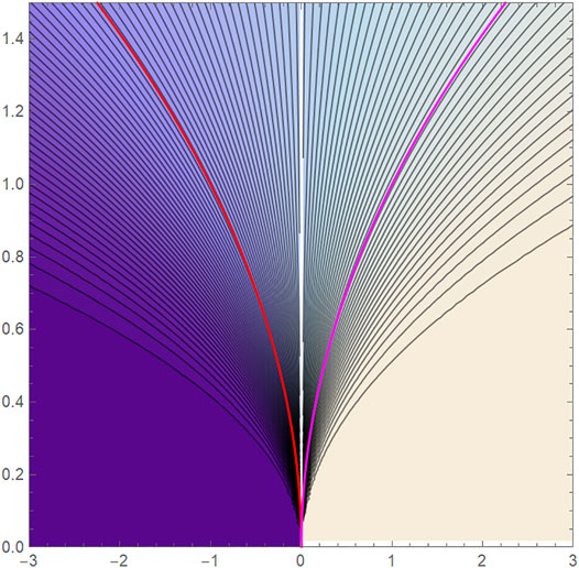
Let us move away from points a certain Riemannian distance from a point and consider the surface and the level sets of $P_Z(\partial \stackrel{̄}{}=A)$. As before, we will normalize A to be 1, and let Z = 0.6. The behavior of $P_Z(\partial \stackrel{̄}{}=A)$ as functions of μ and σ has been analyzed in [13], so we will not repeat the results from there. The plot of $P_{.6}(\partial \stackrel{̄}{}=1)$ is given in Figure 10.

FIGURE 10

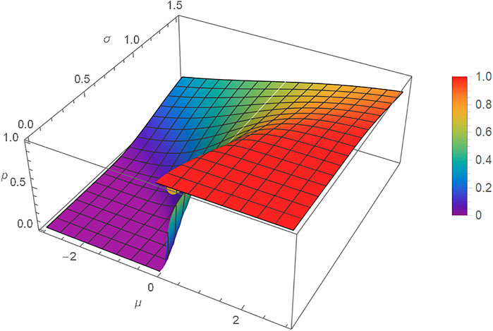
FIGURE 10. Plot of $P_{.6}(\partial \stackrel{̄}{}=1)$ for μ ∈ (−3, 3), σ ∈ (0, 1.5). The limited range is due to the fact that the plot is extremely close to 1 for large μ and small σ. The function is continuous and is equal to 0.6 when μ = 0.

Let us consider the level sets of $P_{.6}(\partial \stackrel{̄}{}=1)$; in fact, this holds for the level sets of $P_Z(\partial \stackrel{̄}{}=A)$ for Z ∈ (0, 1).

Theorem 2. The level sets of $P_Z(\partial \stackrel{̄}{}=1),0<Z<1$ correspond to constant values of μ/σ².

Proof. (⇐) If μ/σ² = μ′/σ′² = k, then it is obvious that $P_Z(\partial \stackrel{̄}{}=1)=\frac{e^{-\frac{2Z\mu }{{\sigma }^2}}-1}{e^{-\frac{2\mu }{{\sigma }^2}}-1}=\frac{e^{-2Zk}-1}{e^{-2k}-1}=\frac{e^{-\frac{2Z{\mu }^{\prime }}{{{\sigma }^{\prime }}^2}}-1}{e^{-\frac{2{\mu }^{\prime }}{{{\sigma }^{\prime }}^2}}-1}$. (⇒) By (16, Cor 3.1), we have that for C > D > 0, that $\frac{e^{-Dk}-1}{e^{-Ck}-1}$ is an increasing function of x. Let C = 2, D = 2Z, we have that $f(k)=\frac{e^{-2Zk}-1}{e^{-2k}-1}$ is an increasing function of k and the result follows. □

Let us look at the level sets of this surface in Figure 11. We see 100 level sets going from left to right in ascending order from 0.01 to 0.99 in approximate steps of 0.01. The middle level set is white and that corresponds to $P_{.6}(\partial \stackrel{̄}{}=1)=.6$ which occurs when μ = 0.

FIGURE 11

FIGURE 11. Level sets of $P_{.6}(\partial \stackrel{̄}{}=1)$, horizontal axis is μ, vertical axis is σ.

Keep in mind that every level set of $P_{.6}(\partial \stackrel{̄}{}=1)$ corresponds to the curve given by μ/σ² = k. For k < 0, we have the level set on the left hand side (LHS) of Figure 11. For k = 0, we have the vertical white line at μ = 0, and for k > 0 we have the level sets on the right hand side (RHS) of Figure 11. Note that we specifically illustrated the level set corresponding to μ/σ² = −1 which is equivalent to $\sigma =-\sqrt{\mu }$ and corresponds to the red level set on the LHS of the figure; and corresponds to $P_{.6}(\partial \stackrel{̄}{}=1)=.363$. We also illustrated the level set corresponding to k = 1, which is the purple curve on the RHS of the figure and corresponds to $P_{.6}(\partial \stackrel{̄}{}=1)=.808$. Of course, now we see why the maximum values that we discussed above are not at μ corresponding to the center of the metric circle, but to the right. This result occurs because the level curve that is tangent to the plot is where the maximum is found. This result can be analyzed with Lagrange multiplier theory, a direction we will pursue in future work. It suffices for this article to show that the trade-off between μ and σ is non-trivial.

4 Impact on Teams and Multi-Agent Systems

We have learned from the mathematics that the decision to attempt to increase skill or to increase interdependence is not trivial. The best answer is a complicated mathematical expression. We also could have looked at the time to obtain the correct answer, but this is even more complicated and will also be addressed in future work.

Presently, our problem boils down to the probability of reaching the correct answer by using the Riemannian distance described in this article—which gets a Team to the highest new probability of success by staying within the distance constraints on skill and interdependence.

Of course, general rules of thumb can be derived by studying the geometry of the question in hand, and near-optimal solutions may be good enough to satisfy a user.

Recall from [16], for μ > 0 (the situations we have been looking into), the lower the diffusion, the greater the interdependence. We note that our mathematics shows that to optimize Team performance, it takes a combination of increasing the drift/skill μ > 0 and lowering the diffusion σ (increasing interdependence) to optimize the probability of the Team of multi-agents of reaching the correct conclusion to a problem that it confronts.

5 Concluding Remarks

Presently, to avoid complicated Riemannian geometric discussions, it is best to use rules of thumb that can be derived from the various plots of the Teams in question. This present work continues the theme emphasized by Lawless [9, 10] of the importance of interdependence, but also has thrown the skill issue into the mathematical mix. This point is not to say that others have ignored skill, rather that their focus was in the interesting and not completely understood topic of interdependence. It was our desire in this article to present a framework incorporating more of the mathematics for decision making.

Future work needs to be done on this topic. We have presented an idealized mathematical model. If the Teams are not simply multi-agents systems, but rather human, or human-machine hybrid teams, our model must be tempered by human factors. Humans do not act as automatons. These ideas are discussed in detail in the beautiful books by Kahneman [6, 7], and also [21]. A good overview of Kahneman’s Nobel prize work in behavioral economics can be found in [5]. In fact, from [7] we can take the concept of noise and view that in terms of diffusion. As we rely more and more on hybrid teams, we must factor in a behavioral economics type approach to Team decision making. How this relates to the mathematics holds promise as a new research area. Furthermore, Teams are often subject to the wisdom of crowds [21], or the stupidity of crowds [19] (this work involves ants, which might be better representative agents than humans when attempting to model a machine), and the mathematical model we have presented does not incorporate such human factors. Of course, future work could include looking at and measuring these factors for an actual Team/MAS.

Data Availability Statement

The original contributions presented in the study are included in the article, further inquiries can be directed to the corresponding author.

Author Contributions

The author confirms being the sole contributor of this work and has approved it for publication.

Conflict of Interest

The author declares that the research was conducted in the absence of any commercial or financial relationships that could be construed as a potential conflict of interest.

Publisher’s Note

All claims expressed in this article are solely those of the authors and do not necessarily represent those of their affiliated organizations, or those of the publisher, the editors and the reviewers. Any product that may be evaluated in this article, or claim that may be made by its manufacturer, is not guaranteed or endorsed by the publisher.

Acknowledgments

We thank Bill Lawless, Ruth Heilizer and the reviewers for their efforts. We are grateful to a reviewer and Ciara Sibley for pointing out, and discussing, the relevant research of Daniel Kahneman.

Footnotes

¹In this article, we had to make a choice between readability for the non-expert in differential geometry and exact precision with respect to Riemannian geometry. We hope that we have achieved a happy middle ground, and we assure the interested reader that any of the missing fine points can be found in the literature (e.g. [20]).

References

1.National Research Council. Enhancing the Effectiveness of Team Science. In: Cooke NJ, and Hilton ML, editors. Committee on the Science of Team Science; Board on Behavioral, Cognitive, and Sensory Sciences; Division of Behavioral and Social Sciences and Education; National Research Council. Washington, DC: The National Academies Press (2015).

Google Scholar

2.Springer. Autonomous Agents and Multi-Agent Systems. Berlin, Germany: Springer Journal (1998-2021).

Google Scholar

3. Feller W. An Introduction to Probability Theory and its Applications, Vols.1&2. Hoboken, NJ, USA: Wiley (1950/1968).

Google Scholar

4. Einstein A. Über die von der molekularkinetischen Theorie der Wärme geforderte Bewegung von in ruhenden Flüssigkeiten suspendierten Teilchen. Ann Phys (1905) 322:549–60. doi:10.1002/andp.19053220806

CrossRef Full Text | Google Scholar

5. Kahneman D. Maps of Bounded Rationality: Psychology for Behavioral Economics. Am Econ Rev (2003) 3(5):14491475. doi:10.1257/000282803322655392

CrossRef Full Text | Google Scholar

6. Kahneman D. Thinking, Fast and Slow. New York, NY, USA: Farrar, Straus and Giroux (2013).

Google Scholar

7. Kahneman D, Olivier S, Cass S. Noise: A Flaw in Human Judgment. New York City: Little, Brown Spark (2021).

Google Scholar

8. Lalley S, Mykland P. Lecture Note Statistics 313: Stochastic Processes II. New York City: Spring (2013). Available from: https://galton.uchicago.edu/lalley/Courses/313/. (Accessed October 13, 2021).

Google Scholar

9. Lawless WF. The Entangled Nature of Interdependence. Bistability, Irreproducibility and Uncertainty. J Math Psychol (2017) 78:51–64. doi:10.1016/j.jmp.2016.11.001

CrossRef Full Text | Google Scholar

10. Lawless WF. The Physics of Teams: Interdependence, Measurable Entropy and Computational Emotion. Front Phys (2017) 2017. doi:10.3389/fphy.2017.00030

CrossRef Full Text | Google Scholar

11. Lawless WF. Quantum-Like Interdependence Theory Advances Autonomous Human-Machine Teams (A-HMTs). Entropy (2020) 22(11):1227. doi:10.3390/e22111227

PubMed Abstract | CrossRef Full Text | Google Scholar

12. Moskowitz IS, Lawless W, Hyden P, Mittu R, Russell S. A Network Science Approach to Entropy and Training. Palo Alto, California, U.S.: AAAI Spring Symposia Series, AAAI Press, 2015.

Google Scholar

13. Moskowitz IS. Agent Team Action, Brownian Motion and Gambler’s Ruin. Eng Artificially Intell Syst (2021) 2021. doi:10.1007/978-3-030-89385-9_6

CrossRef Full Text | Google Scholar

14. Moskowitz IS, Russell S, Lawless W. An Information Geometric Look at the Valuing of Information. In Chapter 9. Human-Machine Shared Contexts. Editors Lawless W. Amsterdam, Netherlands: Elsevier (2020). doi:10.1016/b978-0-12-820543-3.00009-2

CrossRef Full Text | Google Scholar

15. Moskowitz IS, Brown NL, Goldstein Z. A Fractional Brownian Motion Approach to Psychological and Team Diffusion Problems. In: Lawless Wet al. editors. Ch. 11, Systems Engineering and Artificial Intelligence. Berlin, Germany: Springer (2021). doi:10.1007/978-3-030-77283-3_11

CrossRef Full Text | Google Scholar

16. Moskowitz IS. Agent Team Action, Brownian Motion and Gambler’s Ruin. Chaper 11. In: Lawless Wet al. editors. Lecture Notes in Computer Science (LNCS). Berlin, Germany: Springer (2021).

Google Scholar

17. Ratcliff R. A Theory of Memory Retrieval. Psychol Rev (1978) 85(2):59–108.

CrossRef Full Text | Google Scholar

18. Ratcliff R, Smith PL, Brown SD, McKoon G. Diffusion Decision Model: Current Issues and History. Trends Cogn Sci (2016) 20(4):260–81. doi:10.1016/j.tics.2016.01.007

PubMed Abstract | CrossRef Full Text | Google Scholar

19. Sasaki T, Granovskiy B, Mann RP, Sumpter DJ, Pratt SC, Pratta SC. Ant Colonies Outperform Individuals when a Sensory Discrimination Task Is Difficult but Not when it Is Easy. Proc Natl Acad Sci U S A (2013) 110:13769–73. doi:10.1073/pnas.1304917110

PubMed Abstract | CrossRef Full Text | Google Scholar

20. Spivak M. A Comprehensive Introduction to Differential Geometry. Volumes 1-5. 3rd ed. Los Angeles: Publish or Perish (1999).

Google Scholar

21. Surowiecki J. The Wisdom of Crowds. New York City: Anchor (2005).

Google Scholar