- 1Key Laboratory of Ministry of Education for Geomechanics and Embankment Engineering, Hohai University, Nanjing, China
- 2College of Civil Engineering, Nanjing Forestry University, Nanjing, China
- 3School of Computer Science, Nanjing University of Posts and Telecommunications, Nanjing, China
Coral mud is widely distributed in the South China Sea. Studying deformation laws of coral mud is important to the infrastructure development in the South China Sea. In this article, a one-dimensional oedometer test of coral mud under near-natural conditions is performed. The exponential fitting model, Burgers model and ODGM model are used to analyse the time-strain relationship of coral mud under different vertical pressures. The self-fitting accuracy and prediction accuracy of the three models under different vertical pressures are compared. Then, the number of data points used in the model was reduced, and the associated change in accuracy and model stability of the three models were analysed. The study found that the ODGM model has high self-fitting, high prediction accuracy, and a high model stability when the number of data points is reduced, which describe the long-term nonlinear deformation of coral mud more accurately.
1 Introduction
With the continuous exploration and development of the ocean and the construction of related projects such as ports and airports, land resources are becoming increasingly scarce. More available land resources can be obtained by hydraulic fill, which can help alleviate the shortage of coastal land. The settlement and consolidation characteristics of clay have thus become important objects of research. Some researchers [1, 2] suggested that natural settlement can be divided into dispersed free settling, flocculation free settling, zone settling and consolidation settling according to the difference in initial water content, and believes that while the upper soil particles settle, the bottom is also consolidating [3]. designed test equipment that can measure sedimentation, demonstrating more effective research methods. To study the behaviour of clay under constant vertical stress, a one-dimensional oedometer test is typically used to study this time-strain relationship.
Regardless of the field test or laboratory test, the relationship between the deformation of clay under constant vertical stress and time appears to be nonlinear. This deformation, which continues to develop with time, is called creep [4, 5]. Two different hypotheses (A and B) have been used as a basis of discussion to determine whether creep exists in the primary consolidation stage. Hypothesis A purports that creep occurs only after the completion of the primary consolidation settlement stage, such as [6, 7]. Hypothesis B purports that creep exists throughout the consolidation settlement process, as described by [8, 9]. Based on Hypothesis B, various creep constitutive models have been proposed by researchers worldwide [10]. proposed a logarithmic relationship between the vertical stress and the strain under different load durations the one-dimensional oedometer test of normally consolidated soil. Also [11], replaced these e-lgp curves under different load durations with a set of parallel lines called instantaneous compression lines and assumed that these parallel lines of the same distance are 10 times forward. The isotache concept describes the characteristics of long-duration creep behaviour well, but simply treating the e-lgp relationship as a straight line cannot describe the true curves of long-term creep under constant vertical stress [9]. proposed a nonlinear creep equation that considers the limit state and unloading expansion through a multi-staged loading oedometer test that consists of loading and unloading stages. Some researchers proposed a series of fractional order models to analyze the creep of coral sand [12–14]. In addition, many studies have attempted to describe creep behaviour through component models [15], such as the Maxwell model [16] and the Merchant model [17].
Whether using the empirical, component, semiempirical or semitheoretical model, most researchers use the fitting method to analyse the strain-time curve. An accepted data analysis method, the fitting method is simple and convenient but causes experimental data to move closer to a certain artificially prescribed curve shape. The fitting method also yields large differences in accuracy and parameters for different types of soils under different conditions. In addition, the results of laboratory samples are often markedly different than experimental results (e.g. [18], and the fitting parameters obtained through laboratory tests often cannot be directly applied to practical applications. The amount of data from conventional geotechnical tests is not sufficient to support the big data analysis methods that have emerged in recent decades. The small data analysis methods for “less data and poor information” represented by the grey systems theory [19] can be applied to the analysis of these geotechnical test data. Currently, in the geotechnical field, current grey system theory is often used in risk analysis, soil quality assessment [20] and subgrade settlement prediction [21].
In this study, a set of laboratory one-dimensional oedometer tests is used to analyse the time-strain relationship under constant vertical stress using the exponential fitting model, Burgers model and grey model separately. By comparing the advantages and disadvantages of the three models with regard to self-fitting, prediction, and model stability when the number of data is reduced, the possibility of using the grey system to predict long-term nonlinear deformation is analysed. Results show that the grey model method has a significantly better degree of fitting, accuracy and stability when analysing the time-strain curve under different vertical stresses.
2 Material and Test Details
2.1 Material
Corals only grow in warm waters at shallow depths in the tropical ocean between the Tropic of Cancer in the Pacific Ocean, the Indian Ocean, and the Red Sea. Coral mud is an inanimate marine soil mass that is formed by the accumulation of bones and shells of coral populations after a long period of geological action. Due to hydraulic separation, coral mud will appear under the seabed as layers.
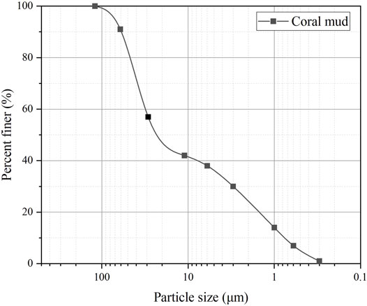
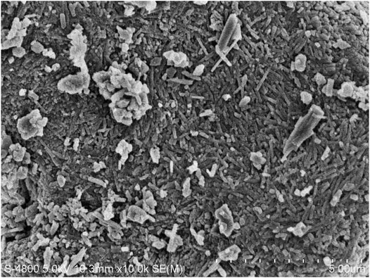
The coral mud investigated in this study is sampled from the South China Sea and has a calcium carbonate content of more than 97%. The properties of the soil are shown in Table 1; Figure 1. The colour of coral mud is white to light yellow; the particles has marked edges and corners; and the particle size distribution is uneven. Scanning electron microscopy (SEM) images of the coral mud are shown in Figure 2 and show that the particles are primarily striped and needle-shaped.
2.2 One-Dimensional Oedometer Test
In this study, a multi-stage loading (MSL) oedometer is employed to investigate the soil behaviour in one-dimensional (1D) conditions. The sample is 20 mm high and 61.8 mm in diameter. Filter paper is attached to the top and bottom of the sample, and drainage stones are placed. A dial gauge with an accuracy of 0.01mm was used to measure the vertical strain. During experiments, the water level in the tank is kept higher than that in the sample to ensure that the sample in the ring cutter is always saturated. The specimens are placed into the steel ring, and the internal surface of the ring is applied with silicone grease to minimize possible friction.
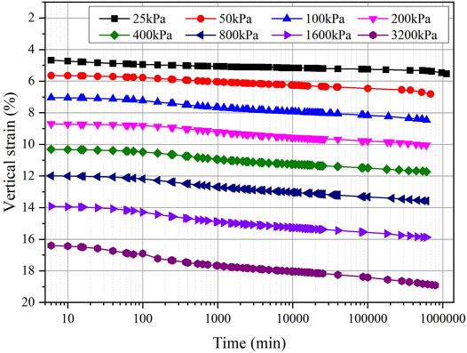
Before the test, the coral mud is dried, ground and sieved to form a soil sample with an initial water content of 45.5%, and the loading ratio of the test is 1. Vertical stresses of 25, 50, 100, 200, 400, 800, 1,600, and 3,200 kPa are applied to the specimen in sequence. The loading time for each level lasted for 8 days, and the loading time for the first and last levels is 14 days to ensure that the specimen had gone through a sufficiently long test. Under different constant vertical stresses, the variations in vertical strain with time are shown in Figure 3.
Figure 3 shows that when the loading ratio is 1, the time-strain relationship curve of each level is similar to the vertical.
3 Creep Model
In this study, the exponential fitting model, Burgers model and grey model were used to analyse the time-strain data of specimens under different vertical stresses.
3.1 Grey Systems Theory
In 1982 [22], first proposed the concept of grey systems theory, which manages uncertain systems with partially known information by generating, mining and extracting useful information from available information. An entire array of new hybrid branches of study, such as grey hydrology, grey geology, grey theory, grey methods of breeding, grey medicine, grey systems analysis of regional economics, etc., have been developed along with the opportunity presented by grey systems theory. In the 1990s, grey systems theory was first applied to the field of soil deformation prediction and was then widely used to predict settlement.
After nearly 40 years of development, the grey model has now developed into a variety of forms to manage different data types. These grey models can be used as independent modules that can be easily used.
3.1.1 GM (1,1) Model
GM(1,1) stands for the first-order grey model in one variable and is the most classic form of the model. Let X(0) = (x(0)(1), x(0)(2), , x(0)(n)) be a sequence of raw data. We denote its accumulation generated sequence by X(1) = (x(1)(1), x(1)(2), , x(1)(n)). Then:
is referred to as the original form of the GM(1,1) model. The original form of the GM(1,1) model is essentially a difference equation, and the parameter vector
Based on the original form of the GM(1,1) model and the model parameters estimated by Eq. 2, the model obtained using the solution of the original difference Eq. 1 as the time response is called the original difference form of the GM(1,1) model, which is called the original differential GM (1,1) model (ODGM).
3.1.2 Application of the Isotache Concept in Grey Model
In the one-dimensional oedometer test, the strain of the soil increases rapidly within a short period of time at the initial stage of load application; with increasing time, the rate of strain increase tends to be slow.
Grey systems theory requires that a grey model be developed based on the original data at equal intervals. When data are obtained from unequal intervals, it is necessary to pre-process the original data through methods such as linear interpolation or an improved grey model. However, these data processing methods will cause errors of varying degrees, thus requiring us to design a better data reading program to avoid unequal reading time intervals as much as possible.
Although the reading programs of commonly used one-dimensional oedometer tests are different, most follow the law that the reading interval gradually increases as the time of vertical load acting on the specimen increases.
Combining the related assumptions of the isotache concept [23], this paper redesigned the reading program. The new reading method is to read according to equal logarithmic time interval (i.e., to read when lg t = 0.8, 1, 1.2, …). The new reading program can ensure that the reading data can be used in the model directly, which avoids errors during pre-processing.
3.2 Empirical Model
An empirical model is simple and easy to use but only sums up equations from data and lacks theoretical guidance. The physical meaning of an empirical models parameters may also not be clear. In addition, the parameters of different specimens vary markedly under different conditions, and model generality is poor.
In this article, the simplest and most commonly used exponential fitting is used for comparative analysis, and the fitting equation is:
where A1, t1 and y1 are the fitting parameters of the exponential fitting model.
3.3 Component Model
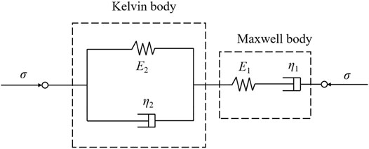
When selecting a component model to describe the long-term nonlinear relationship of the soil, the number of parameters should be minimized to improve accuracy. This paper uses the Burgers model as a comparison model that consists of a Kelvin body and a Maxwell body connected in series (Figure 4), which can describe the three stages of instant deformation, decay deformation and steady deformation during deformation [24].
The constitutive equation of Burgers model is:
where E1 is the elastic modulus of the Maxwell body and E2 is the elastic modulus of the Kelvin body. When the vertical stress σ is constant, Eq. 5 can be written as:
where
When t → ∞,
In the Burgers model, the instant deformation after loading is only related to E1, while the decay deformation and steady deformation are related to E2, η1 and η2.
For any t ≥ 0, ɛ′′(t) < 0. This means that the delay deformation rate will continue to decrease with increasing time and continue to tend to
4 Test Results and Discussion
A total of 20 reading points in 6 s–11 h 5 min under 8 different vertical stresses were used to establish exponential fitting, Burger model and ODGM model, respectively, and the strain within 27 h 47 min-175 h 15 min was predicted. Thus, for a specimen under a constant vertical pressure, the strain of approximately 175 h is predicted through the data of the first 11 h, and the predicted data obtained through the models are compared with the real data of the test.
The vertical strain of the test data and the three models with time is shown in Figure 5.
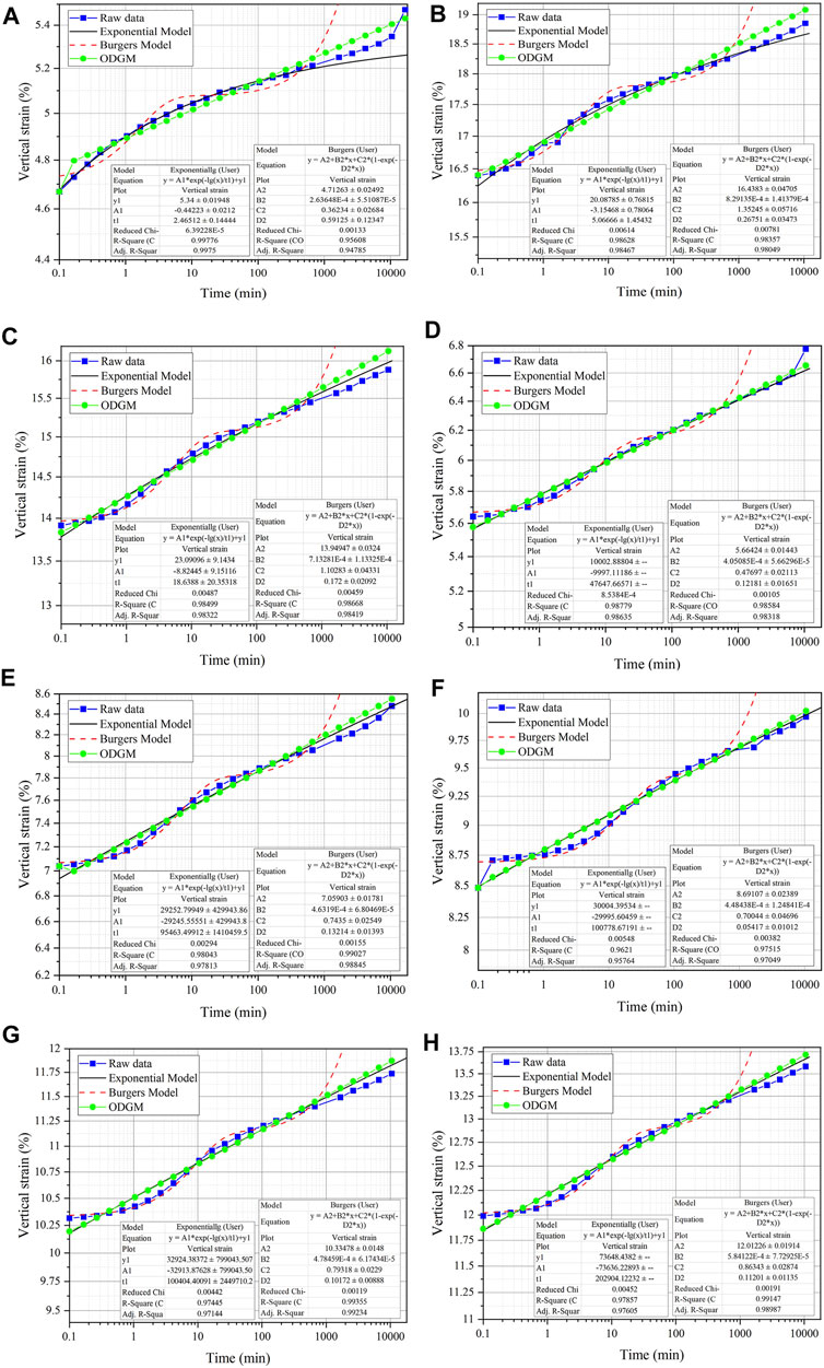
FIGURE 5. Relationship of vertical strain and time (log-scale) and prediction results of three models under different vertical stresses.(textbf(A) σ =25 kPa, textbf(B) σ =50 kPa, textbf(C) σ =100 kPa, textbf(D) σ =200 kPa, textbf(E) σ =400 kPa, textbf(F) σ =800 kPa, textbf(G) σ =1600 kPa, textbf(H) σ =3200 kPa)
4.1 Model Self-Fitting
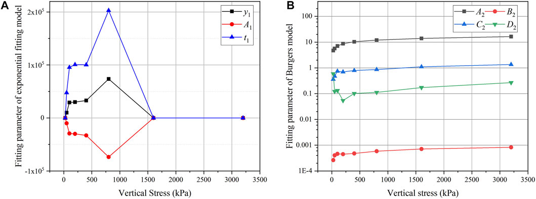
The self-fitting parts of the exponential fitting model, Burgers model and ODGM model are analysed, and the fitting parameters of the exponential fitting model under different constant vertical stresses are shown in Figure 6A.
Figure 6A shows that the parameters of exponential fitting under different vertical stresses exhibit no strong trends, and there are large differences between the parameters. These results show that under different vertical pressures, the shape of the curve obtained by exponential fitting is not always similar. Some fitting parameters of the exponential fitting model are large both in magnitude and in confidence interval, which makes the model have a higher risk of instability.
The fitting parameters of the Burgers model are shown in Figure 6B.
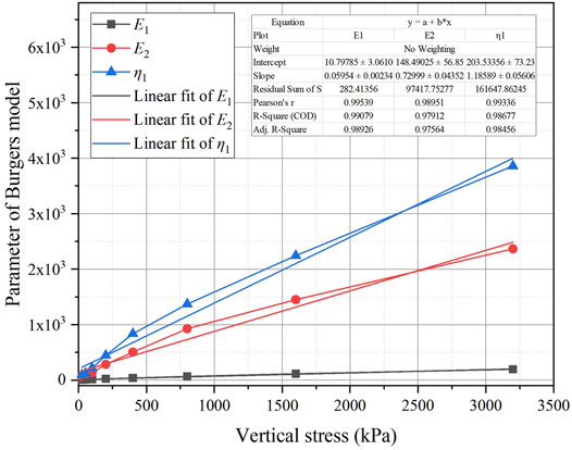
The parameters of the Burgers model are generally regular. As the vertical pressure increases, E1, E2, and η1 also increase and show a higher linear correlation, as shown in Figure 7.
The ODGM model does not set parameters; thus, there is no need to discuss changes in model parameters. For each model, we define the average absolute error Δ, then:
where x(i) is the calculated value of the model and xa(i) is the real reading value. The average absolute error between the calculated value and the real value of the model within 6 s–11 h 5 min is shown in Figure 8.
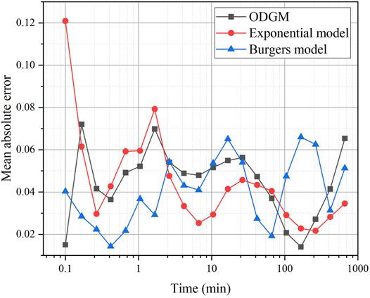
FIGURE 8. Relationship of mean absolute error and time (log-scale) of three models in the process of self-fitting.
Figure 8 shows that all three models have good self-fitting accuracy. After approximately 1 h of loading, the relative error of the three models fluctuates similarly, and the self-fitting error is larger at the point of maximum curvature of the original data curve in this time period.
Compared with the two other models, the Burgers model can describe the deformation at the initial stage after loading accurately.
As the loading time increases, the exponential fitting model can express the subsequent deformation better, and its fitting curve tends to be straight. However, the fitting curve that approximates a straight line cannot describe the change in the initial stage of loading. In addition, the parameter values and confidence intervals obtained by the fitting are too large, which makes the model at risk of instability.
The ODGM has the advantages of both: errors are relatively smoothly distributed in a small range throughout the stage, and possible defects of the fitting method are avoided.
4.2 Model Prediction
Using the exponential fitting model and Burgers model parameters obtained via self-fitting in Section 4.1 and continuing to calculate the ODGM sequence obtained in 4.1, the predicted values of the three models at the subsequent prediction points 27 h 47 min-277 h 47 min are obtained. The average absolute error Δ between the predicted values of the three models and the real readings is shown in Figure 9.
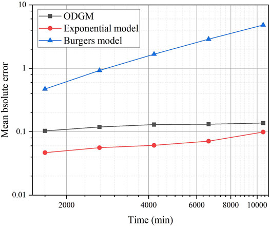
FIGURE 9. Relationship of mean absolute error and time (log-scale) of three models in the process of prediction.
Figure 9 shows that when predicting the long-term deformation, the average absolute error between the exponential fitting model and the ODGM model is generally within 0.15, and the average absolute error of the Burgers model is relatively large, which means that the model fails rapidly.
The Burgers model has a high degree of fit in the early self-fitting stage and can better describe the characteristics of the double S-shaped curve of the time-strain relationship, but the error between the predicted value and real value increases rapidly when the self-fitting curve is extended. Therefore, the model is not suitable for model prediction but is more suitable for analysis of the entire process of vertical strain-time.
Although the exponential fitting model achieves a high prediction accuracy, its predicted value may be larger or smaller than the real data under different vertical stresses. It is impossible to determine whether the prediction result is safe or biased. In practical engineering applications, this prediction result is unfavourable. In the fitting process of strain-time relations under different vertical stresses in this paper, the fitting curves with higher prediction accuracy are shown in Figures 5B–F, and the fitting parameter values are all large. This results indicates that the fitting curve of the exponential fitting model tends to be straight and cannot describe the double S-shaped curve characteristics of the time-strain relationship.
In general, the ODGM yields higher accuracy and more stable changes in error during self-fitting and prediction, and can also ensure that the prediction results are in the area with larger real values, ensuring the safety of the prediction results in practical applications.
4.3 Model Prediction With Reduced Data Points
To further compare the stability and prediction accuracy of the three models, based on Section 4.2, the data used by the model were reduced, and the number of data involved in the model fitting were reduced from 6 s to 11 h 5 min (20 data points in total) to 6 s- 2 h 46 min (17 data points in total) and 6 s- 41 min (14 data points in total). ODGM model calculation, Burgers and exponential fitting model fitting were performed, and predictions were made. The fitting and prediction results are shown in Figure 10.
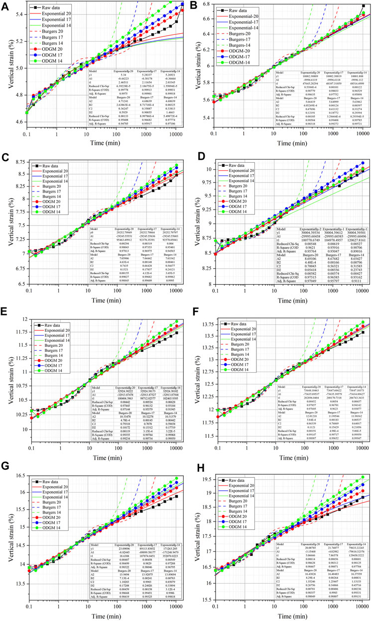
FIGURE 10. Relationship of vertical strain and time (log-scale) and prediction results of three models under different vertical stresses (20 data points/17 data points/14 data points). (textbf(A) σ =25 kPa, textbf(B) σ =50 kPa, textbf(C) σ =100 kPa, textbf(D) σ =200 kPa, textbf(E) σ =400 kPa, textbf(F) σ =800 kPa, textbf(G) σ =1600 kPa, textbf(H) σ =3,200 kPa).
4.3.1 Model Self-Fitting With Reduced Data Points
As the number of data points used for self-fitting decreased, the average absolute error Δ under different vertical stresses is shown in Figure 11.
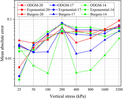
FIGURE 11. Relationship of mean absolute error and vertical press (log-scale) of three models (20 data points/17 data points/14 data points)
As the number of data points involved in the model was reduced, the self-fitting accuracy of the three models remained good. The average absolute error of the Burgers model and the exponential fitting model fluctuated sharply, while the ODGM fluctuated relatively smoothly.
The self-fitting accuracy of the exponential fitting model was marginally reduced, and the self-fitting accuracy of the Burgers model was markedly improved by reducing the number of data points. This result again demonstrates that the Burgers model can more accurately describe deformation at the initial stage of loading, while the exponential fitting model is better at describing the long-term deformation after loading. The variation in the mean absolute error of the ODGM is small throughout the stage, indicating that the model is stable.
The parameter changes of the exponential fitting model with reduced data points are shown in Figure 12A.
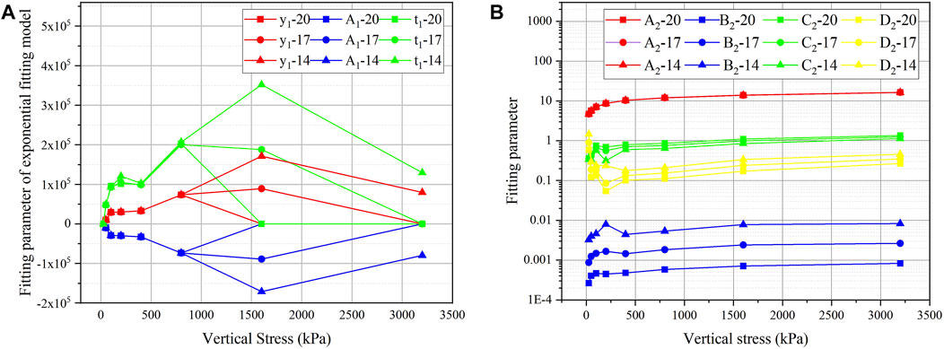
FIGURE 12. Exponential fitting parameters under different vertical stresses (20 data points/17 data points/14 data points)). (A) is exponential, (B) is Burgers.
The changes in the parameters of the exponential fitting model are more chaotic. Compared with Figure 6A, the parameters vary markedly with the change in vertical pressure, but the parameters of the data under the same vertical stress will also change markedly with the reduction in the number of data points involved, as shown in Figures 10G,H. This result shows that the exponential fitting model has poor stability.
As shown in Figure 12B, the parameter changes of the Burgers model exhibit strong trends. As the number of data points decreased, A and C decreased, while B and D increased. The changes in these parameters are maintained within a small range.
4.3.2 Model Prediction With Reduced Data Points
The cumulative absolute error between the predicted value and the real value of the strain obtained under different vertical pressures in different prediction methods is shown in Figure 13.
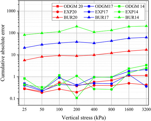
FIGURE 13. Relationship of mean absolute error and vertical stress (log-scale) of three models in the process of prediction (20 data points/17 data points/14 data points).
Figure 13 shows that as the forecast data decreased, with the reduction in data points, the cumulative absolute error of prediction between the exponential fitting model and ODGM model remained in a relatively low range, while the cumulative absolute error of the Burgers model increased rapidly.
Observing the cumulative error of the exponential model fitting and the ODGM model, the cumulative absolute error was found to fluctuate more severely, which indicates that the instability of the prediction gradually increases.
The average absolute error of each model at the prediction point under different vertical stresses is shown in Figure 14.
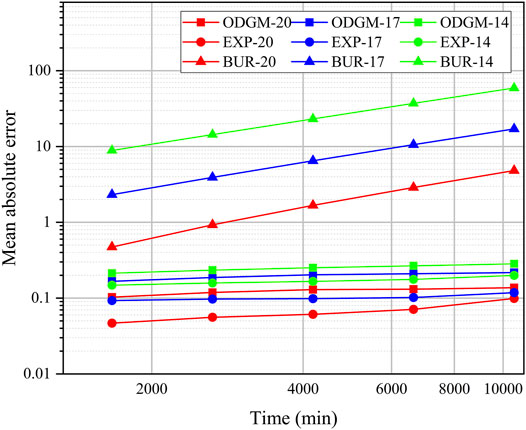
FIGURE 14. Relationship of mean absolute error and time (log-scale) of three models in the process of prediction (20 data points/17 data points/14 data points).
When the number of data points involved in the model decrease, the error of the Burgers model increased markedly and quickly failed. These results further demonstrate that although the model yields a high self-fitting accuracy, it is not suitable for prediction.
Compared with Section 4.2, the shortcomings of the instability of the exponential fitting model are stronger. Although this model yields marginally higher accuracies, its parameters have a wide range of change, and the parameters may also change drastically when the number of data points are reduced, as shown in Figures 10G,H. For the same data, when the model is fitted with fewer data points, its predicted trend may swing up and down the measured value, as shown in Figures 10D,H.
The error of the ODGM method is small, and the error increase is still small as the number of data points decreases. The predicted values are always marginally higher than the real values; thus, the predicted values of the model will be in a safe range in real engineering applications.
5 Conclusion
In this study, an exponential fitting model, Burgers model and ODGM model are developed for the one-dimensional oedometer test of coral mud in the South China Sea. The strain-time model under different vertical pressures is established, and the influence of a reduced number of data points involved in the model is considered. The accuracy, parameter changes and model stability of the three models are analysed. The conclusions of this study are as follows:
1. During the self-fitting process, all three models yield high accuracies. The parameters of the Burgers model exhibit certain trends, but the parameters of the exponential fitting model exhibit none. The grey systems theory model represented by ODGM avoids the appearance of parameters and avoids errors caused by artificial linearity during the fitting process, which is a more modern and scientific model.
2. During prediction, the Burgers model quickly fails, and the prediction accuracies of the exponential fitting model and the ODGM model are high. The predicted value of the exponential model fluctuates around the real value, while the predicted value of the ODGM model is stable in a safe range.
3.The ODGM model produces a high self-fitting and prediction accuracies but can also predict soil deformation when the reading time is tens of times the reading time within a few hours and can ensure sufficient model accuracy.
In future research, the grey model should be introduced to better describe the long-term nonlinear time-strain relationship of the soil under a certain vertical pressure. By introducing the grey model into the three-dimensional constitutive model, the long-term nonlinear deformation characteristics related to time can be described more accurately and conveniently.
Data Availability Statement
The raw data supporting the conclusions of this article will be made available by the authors, without undue reservation.
Author Contributions
HW and YS conceived the research. JD conducted part of tests. J-HX collected the data. KM programmed the model and did the calculations. HW and KM wrote the article with input from all authors.
Funding
This work is supported by the National Natural Science Foundation of China under Grant 51979087.
Conflict of Interest
The authors declare that the research was conducted in the absence of any commercial or financial relationships that could be construed as a potential conflict of interest.
Publisher’s Note
All claims expressed in this article are solely those of the authors and do not necessarily represent those of their affiliated organizations, or those of the publisher, the editors, and the reviewers. Any product that may be evaluated in this article, or claim that may be made by its manufacturer, is not guaranteed or endorsed by the publisher.
References
1. Imai G. Settling Behavior of clay Suspension. Soils and Foundations (1980) 20:61–7710. doi:10.3208/sandf1972.20.2_61
2. Imai G. Experimental Studies on Sedimentation Mechanism and Sediment Formation of clay Materials. Soils and Foundations (1981) 21:7–20. doi:10.3208/sandf1972.21.7
3. Alexis A, Bras GL, Thomas P. Experimental Bench for Study of Settling-Consolidation Soil Formation. Geotechnical Test J (2004) 27:557–67. doi:10.1520/GTJ11582
4. Graham J, Crooks JHA, Bell AL. Time Effects on the Stress-Strain Behaviour of Natural Soft Clays. Géotechnique (1983) 33:327–40. doi:10.1680/geot.1983.33.3.327
5. Zhu QY, Yin ZY, Hicher PY, Shen SL. Nonlinearity of One-Dimensional Creep Characteristics of Soft Clays. Acta Geotechnica (2016) 11:1–14. doi:10.1007/s11440-015-0411-y
6. Ladd C, Foott R, Ishihara K, Schlosser F, Poulos H. Stress-deformation and Strength Characteristics: State of the Art Report. Int J Rock Mech Mining Sci Geomechanics Abstr (1977) 15:26.
7. Mesri G, Godlewski PM. Time- and Stress-Compressibility Interrelationship. J Geotech Engrg Div (1977) 103:417–30. doi:10.1061/ajgeb6.0000421
8. Yin J-H. Non-linear Creep of Soils in Oedometer Tests. Géotechnique (1999) 49:699–707. doi:10.1680/geot.1999.49.5.699
9. Feng W-Q, Lalit B, Yin Z-Y, Yin J-H. Long-term Non-linear Creep and Swelling Behavior of hong kong marine Deposits in Oedometer Condition. Comput Geotechnics (2017) 84:1–15. doi:10.1016/j.compgeo.2016.11.009
10. Crawford CB. Interpretation of the Consolidation Test. J Soil Mech Found Div (1964) 90:87–102. doi:10.1061/jsfeaq.0000664
11. Bjerrum L. Engineering Geology of Norwegian Normally-Consolidated marine Clays as Related to Settlements of Buildings. Géotechnique (1967) 17:83–118. doi:10.1680/geot.1967.17.2.83
12. Sun Y, Chen C. Fractional Order Creep Model for Coral Sand. Mech Time-depend Mater (2019) 23:465–76. doi:10.1007/s11043-018-9400-5
13. Sun Y, Sumelka W. Fractional Viscoplastic Model for Soils under Compression. Acta Mech (2019) 230:3365–77. doi:10.1007/s00707-019-02466-z
14. Sun Y, Sumelka W. Multiaxial Stress-Fractional Plasticity Model for Anisotropically Overconsolidated clay. Int J Mech Sci (2021) 205. doi:10.1016/j.ijmecsci.2021.106598
16. Zhang YP, Gao F. Analytical Solution of 1-d Viscoelastic Consolidation of Soft Soils with Fractional maxwell Model. Amm (2012) 157-158:419–23. doi:10.4028/www.scientific.net/amm.157-158.419
17. Ye S, Xue Y, Wu J, Li Q. Modeling Visco-Elastic-Plastic Deformation of Soil with Modified Merchant Model. Environ Earth Sci (2012) 66:1497–504. doi:10.1007/s12665-011-1389-x
18. Larsson R, Mattsson H. Settlements and Shear Strength Increase below Embankments. In: Tech. Rep. Linköping: Swedish Geotechnical Institute (2003).
19. Liu SF, Lin Y. Grey Systems (Understanding Complex Systems). Berlin, Germany: Springer Berlin Heidelberg (2010).
20. Zhang L, Ren L, Tong J, Shi Y. Study of Soil-Solid Adhesion by Grey System Theory*. Prog Nat Sci (2004) 14:119–24. doi:10.1080/10020070412331343241
21. Liu HB, Xiang YM, Nguyen HH. A Multivariable Grey Model Based on Background Value Optimization and its Application to Subgrade Settlement Prediction. Appl Mech Mater (2013) 256-259:1721–5. doi:10.4028/www.scientific.net/AMM.256-259.1721
23. Bjerrum L. Embankments on Soft Ground. In: Performance of Earth and Earth-Supported Structures (1972).
24. Liu QB, Wang S, Xia DS, Xiang W, Su AJ, Wang JE, et al. Experimental Study of Residual-State Creep Behavior of Intact Sliding-Zone Soil. Rock Soil Mech (2017) 38:1305–13.
Keywords: creep, grey model, deformation prediction, oedometer test, coral mud
Citation: Weng H, Shen Y, Deng J, Xu J-h and Ma K (2022) Application of the Grey Model in One-Dimensional Long-Term Creep Analysis of Coral Mud From the South China Sea. Front. Phys. 10:835933. doi: 10.3389/fphy.2022.835933
Received: 15 December 2021; Accepted: 01 March 2022;
Published: 22 March 2022.
Edited by:
Wanqing Shen, Université de Lille, FranceCopyright © 2022 Weng, Shen, Deng, Xu and Ma. This is an open-access article distributed under the terms of the Creative Commons Attribution License (CC BY). The use, distribution or reproduction in other forums is permitted, provided the original author(s) and the copyright owner(s) are credited and that the original publication in this journal is cited, in accordance with accepted academic practice. No use, distribution or reproduction is permitted which does not comply with these terms.
*Correspondence: Yang Shen, c2hlbnlhbmcxOTk4QDE2My5jb20=
 He Weng1
 Yang Shen
 Jun-hong Xu
