Dehazing Based on Long-Range Dependence of Foggy Images

Deep neural networks (DNNs) with long-range dependence (LRD) have attracted more and more attention recently. However, LRD of DNNs is proposed from the view on gradient disappearance in training, which lacks theory analysis. In order to prove LRD of foggy images, the Hurst parameters of over 1,000 foggy images in SOTS are computed and discussed. Then, the Residual Dense Block Group (RDBG), which has additional long skips among two Residual Dense Blocks to fit LRD of foggy images, is proposed. The Residual Dense Block Group can significantly improve the details of dehazing image in dense fog and reduce the artifacts of dehazing image.

Introduction

The single image dehazing based on deep neural networks (DNNs) refers to restoring an image from a foggy image using DNNs. Although some efforts on dehazing have been proposed recently [1–6], foggy image modeling is still an unsolved problem.

The early image model is Gaussian or Mixture Gaussian [7], but it cannot properly fit with foggy images. In fact, the foggy images seem to show long-range dependence. That is, the gray levels seemed to influence pixels in nearby regions. In our framework, each foggy image with m rows and n columns in SOTS is reshaped as is an m×n column vector by arranging the elements of the image column by column. Thus, we can fit the images by fractional Gaussian noise (fGn) [8–12] and discuss dependence of an image by its Hurst parameter. The main conclusion of the Hurst parameter of a fGn is as follows.

The auto-correlation function (ACF) of fGn is as follows:

$C_{fGn}\left(\tau \right)=\frac{V_H}{2}\left[{\left(\left|\tau \right|+1\right)}^{2H}+{\left(\left|\tau \right|-1\right)}^{2H}-2{\left|\tau \right|}^{2H}\right](1)$

where

$V_H=\Gamma \left(1-2H\right)\frac{\mathit{cos}\mathbf{\pi }\mathbf{H}}{\mathit{\pi }\mathit{H}}(2)$

is the strength of fGn and 0 < H < 1 is the Hurst parameters [8–10].

If 0.5 < H < 1, one has the following:

$\underset{0}{\overset{\infty }{{\displaystyle \int }}}{C}_{fGn}\left(\tau \right)d\tau =\infty (3)$

Thus, the fGn is of long-range dependency (LRD) when 0.5 <H < 1.

When 0 <H < 0.5, one has the following:

$\underset{0}{\overset{\infty }{{\displaystyle \int }}}{C}_{fGn}\left(\tau \right)d\tau <\infty (4)$

The above fGn is of short-range dependence (SRD) [8–12].

Recently, some deep neural networks (DNN) with LRD are proposed [4–6, 13], whose motivation is mainly from avoiding gradient disappearance in training. However, the LRD of these DNNs has never been discussed and proven in theory. In this study, the Hurst parameters of test images in SOTS datasets [14] are computed and LRD of foggy images is proven. Motivated by LRD of foggy images, we proposed a new network module, the Residual Dense Block Group (RDBG) composed of two bundled Residual Dense Block Groups (DRBs) proposed in reference [13]. The RDBG has additional long skips between two DRBs to fit LRD of foggy images and can be used to form a new dehazing network. This structure can significantly improve the quality of dehazing images in heavy fog.

The remainder of this article is as follows: the second section introduces the preliminaries of fGn; the third section gives the case study; then a framework based on LRD of foggy images is presented; finally, there are the conclusions and acknowledgments.

Preliminaries

Fractional Brownian Motion

The fBm of Weyl type is defined by [8].

$B_H\left(t\right)-B_H\left(0\right)=\frac{1}{\Gamma \left(H+0.5\right)}\left\{\underset{-\infty }{\overset{0}{{\displaystyle \int }}}\left[{\left(t-u\right)}^{H-0.5}-{\left(-u\right)}^{H-0.5}\right]dB\left(u\right)+\underset{0}{\overset{t}{{\displaystyle \int }}}{\left(t-u\right)}^{H-0.5}dB\left(u\right)\right\}(5)$

where 0 <H < 1, and B(t) is Gaussian.

$\mathrm{fBm}\mathrm{has}\mathrm{stationary}\mathrm{increment}:B_H\left(t+\tau \right)-B_H\left(t\right)=B_H\left(\tau \right)-B_H\left(0\right)(6)$

$\mathrm{a}\mathrm{n}\mathrm{d}\mathrm{s}\mathrm{e}\mathrm{l}\mathrm{f}\text{-}\mathrm{a}\mathrm{f}\mathrm{f}\mathrm{i}\mathrm{n}\mathrm{i}\mathrm{t}\mathrm{y}\mathrm{p}\mathrm{r}\mathrm{o}\mathrm{p}\mathrm{e}\mathrm{r}\mathrm{t}\mathrm{y}:B_H\left(at\right)=a^H{B}_H\left(t\right),a>0(7)$

Fractional Gaussian Noise

Let x(t) be the gray level of the tth pixel of an image and be a fGn [8–12].

$x\left(t\right)=B_H\left(t\right)-B_H\left(0\right)(8)$

Its ACF follows Eqs 1, 2.

An approximation of C_fGn $\left(\mathrm{\tau }\right)$ is as follows:

${\mathrm{C}}_{\mathrm{f}\mathrm{G}\mathrm{n}}\left(\mathrm{\tau }\right)\propto {\left|\mathrm{\tau }\right|}^{\mathrm{2}\mathrm{H}-2}(9)$

Case Study

Data Set

Synthetic data set RESIDE: Li et al. [16] created a large-scale benchmark data set RESIDE composed of composite foggy images and real foggy images.

Synthetic data set: the SOTS test data set is used as the test set. The SOTS test set includes 500 indoor foggy images and 500 outdoor foggy images.

Real data set: it includes 100 real foggy images in the SOTS data set in the RESIDE and the real foggy data collected on the Internet.

Calculate Hurst Parameter

Rescaled range analysis (RRA) [15] for foggy images is closely associated with the Hurst exponent, H, also known as the “index of dependence” or the “index of long-range dependence.” The steps to obtain the Hurst parameter are as follows:

1. Preprocessing: An image with m row and n column is concatenated column by column to form an m×n column vector. For better understanding, a simple example is presented: the size of the foggy image in Figure 4A is 348×248, and then it is concatenated column by column to form an 86,304-column vector.

2. Rescale vector: The original vector can be divided equally into several ranges for further RRA, as follows. The first range at the first layer is defined as RS₁₁, representing the original m×n vector, and then it can be divided into two parts, RS₂₁ and RS₂₂, at the second layer, whose dimension equals to (m×n/2) where (.) represents the floor integer. Repeat the above process until the vector dimensions at a specific layer are less than (m×n/$2^6$).

Layer 1. RS₁₁: original m×n vector.

Layer 2. RS₂₁: (m×n/2), RS₂₂: (m×n/2).

Layer 3. RS₃₁: (m×n/4), RS₃₂: (m×n/4), RS₃₃: (m×n/4), RS₃₄: (m×n/4).

Thus, the dimensions of ranges of the foggy image are as follows:

Layer 1. RS₁₁: 86,304.

Layer 2. RS₂₁: 43,152, RS₂₂: 43,152.

Layer 3. RS₃₁: 21,576, RS₃₂: 21,576, RS₃₃: 21,576, RS₃₄: 21,576.

3. Calculate the mean for each range.

$m_{ij}=\frac{1}{n_{ij}}{\displaystyle \sum _{k_{ij}=1}^{n_{ij}}{X}_{k_{ij}}}(10)$

where $n_{ij}$ represents the number of the elements in the jth range of the ith layer; $X_{k_{ij}}$ represents the value of the $k_{ij}$ ^th element in the jth range of the ith layer; $m_{ij}$ represents the mean value of the elements in the jth range of the ith layer.

4. Calculate the deviations of each element in every range. The deviation can be calculated as follows:

$Y_{k_{ij}}=X_{k_{ij}}-m_{ij}(11)$

where $Y_{k_{ij}}$ represents the deviation of the $k_{ij}$ ^th element in the jth range of the ith layer.

5. Obtain the accumulated deviations for each element in the corresponding range.

$y_{ij,N}={\displaystyle \sum _{k_{ij}=1}^N{Y}_{k_{ij}}}, N=1,\dots n_{ij}(12)$

where $y_{ij,N}$ represents the accumulated deviation for N elements in the jth range of the ith layer.

6. Calculate the widest difference of the deviations in each range.

$R_{ij}=\mathit{max}\left(y_{ij,1},y_{ij,2}\dots y_{ij,N}\right)-\mathit{min}\left(y_{ij,1},y_{ij,2}\dots y_{ij,N}\right), N=1,\dots ,n_{ij}(13)$

where $R_{ij}$ represents the widest difference for the jth range of the ith layer.

7. Calculate the rescaled range for each range.

$\text{Rescaled range}={\left(\frac{R}{S}\right)}_{ij}=\frac{R_{ij}}{{\sigma }_{ij}}(14)$

where R/S represents the rescaled range for the jth range of the ith layer, while σ_ij represents the standard deviation of the accumulated deviations for the jth range of the ith layer.

8. Obtain the averaged rescaled range values for each layer.

${\left(\frac{R}{S}\right)}_i=\frac{1}{2^{l-1}}{\displaystyle \sum _{j=1}^{\left[m\times n/2^{l-1}\right]}{\left(\frac{R}{S}\right)}_{ij}}(15)$

where l is the layer of the ranges with the identity size. The R/S is calculated using Eq. 15 and the R/S of the example image is shown in Table 1.

9. Obtain the Hurst exponent. Plot the logarithm of the size (x axis) of each range in the ith layer versus the logarithm of the average rescaled range of the corresponding layer using Eq. 15 (y axis) (Figure 1), and the slope of the fitted line is regarded as the value of the Hurst exponent, that is, the Hurst parameter.

TABLE 1

TABLE 1. Some intermediate results of calculating the Hurst parameter of the foggy image in Figure 5A.

FIGURE 1

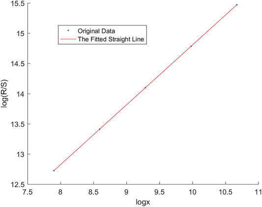
FIGURE 1. Data in the third column (x axis) and the fifth column (y axis) in Table 1 and their fitting straight line whose slope is 0.990.

Hurst Parameters H of Foggy Images

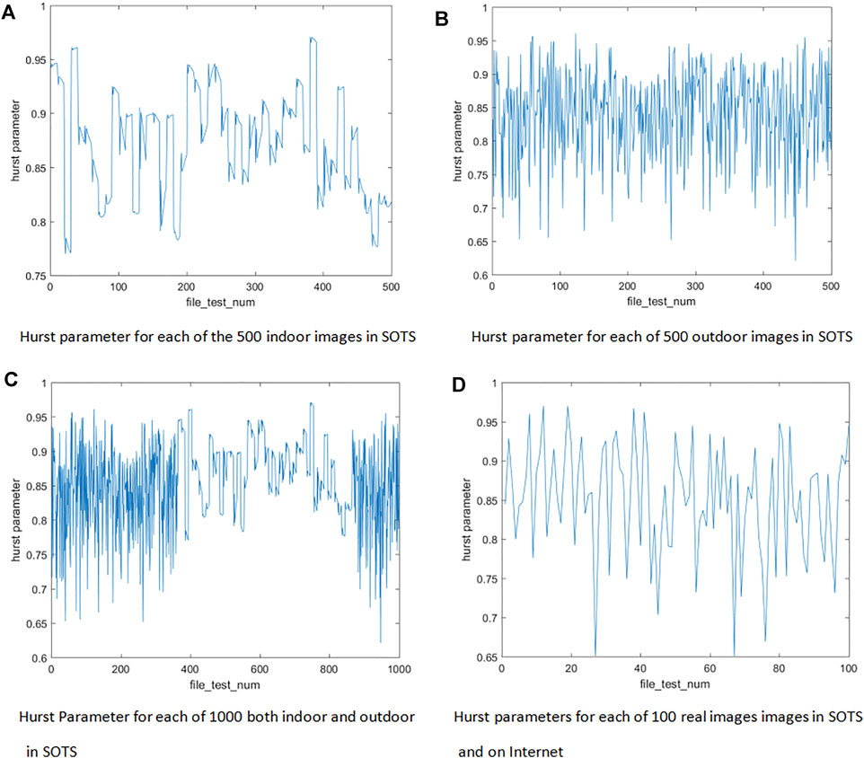
The plots of four image sets in SOTS, 500 indoor images, 500 outdoor, 1,000 outdoor and indoor images, and 100 real foggy images, are shown in Figure 2. The x axis represents the serial numbers of the test images while the y axis is the Hurst parameters of the images. That is, the ith point in Figure 2 represents the Hurst parameter of the ith image. Thus, we can know the Hurst parameters of over 1,000 foggy images by observing y values of the points in Figure 2.

FIGURE 2

FIGURE 2. Plots of H of four foggy image datasets.

From Figure 2, we can observe that the least y values of subfigures in Figure 2 are 0.6 or 0.65, which means that the Hurst parameters of four image data sets are all above 0.6. Thus the foggy images are of LRD, which can help us design some novel dehazing methods.

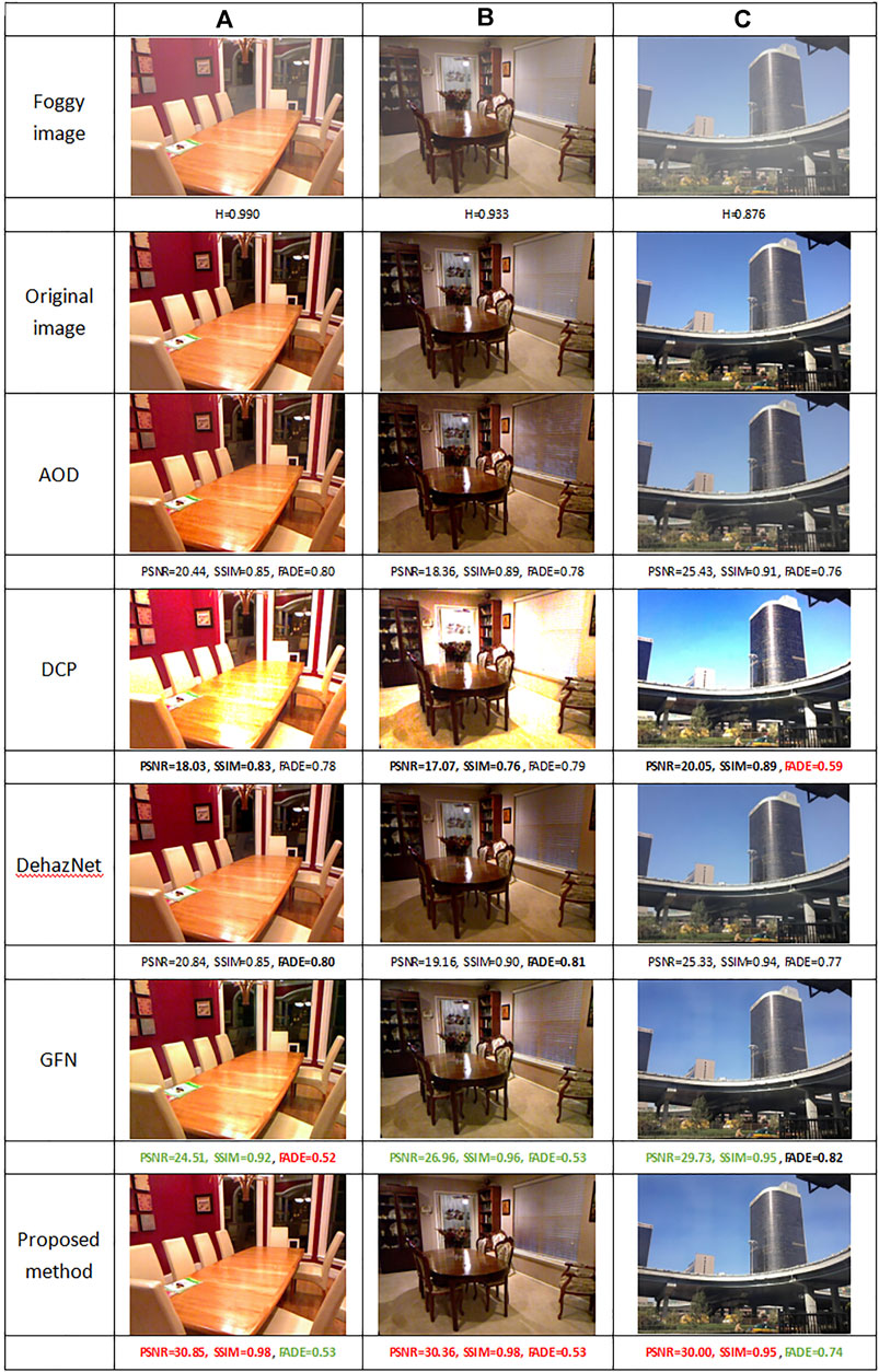
Moreover, although the Hurst parameter for each image is a constant, the different images have different Hurst parameters because of their different contents. For example, the Hurst parameter of a complex image with more colors and objects (Figures 5A,B) is bigger than a simple image (Figure 5C).

Based on the LRD of the foggy images, the Residual Dense Block Group (RDBG) based on RDB is proposed. The RDBG, which has additional long skips between two RDBs to fit LRD of foggy images, can significantly improve the details of dehazing image in dense fog and reduce the artifacts of dehazing image.

Dehazing Based on Residual Dense Block Group

Dependence in Neural Network

The neural network can be considered as a hierarchical graph model whose nodes are connected by weighted edges. The weights of edges are trained according to some predefined cost functions. Generally, the value of the ith node in the kth layer is decided by the nodes in the (k-1)th layer connected to the ith node [18–24]. That is,

$x^{\left(k\right)}\left(i\right)=f\left(W^{\left(k-1,k\right)}\left(i\right)x^{\left(k-1\right)}\left(i\right)\right)(16)$

where $x^{\left(k\right)}\left(i\right)$ is the value of the ith node in the kth layer, f is an activation function, $W^{\left(k-1,k\right)}$ is a vector of weights of edges to connect nodes in the (k-1)th layers and the ith node, and $x^{\left(k-1\right)}\left(i\right)$ are values of nodes in the (k-1)th layers connected to the ith node.

Thus, the value of the ith node is only influenced by its directly connected nodes. This assumption may be correct in some cases, but it is not true in images since we have proved the LRD of foggy images. Thus, we should design a new module of the neural network to fit the LRD of the foggy images.

Residual Dense Block Group

Just as discussed in the above subsection, the most straight method to design a structure fitting LRD of images is to connect a node to nodes with longer distance to it directly. Thus, the information of faraway nodes is introduced to help us to recover the real gray level from foggy observations.

Following this intuitive explanation, the length of a skip (connection edge between two nodes) which is defined as the number of crossing nodes can be used to measure the dependence of a time series approximately.

In this context, motivated by the LRD of foggy images, a new residual module RDBG is proposed by two bundled resident dense blocks (RDBs). As shown in Figure 3A, the RDB is a module with dense connections only in the block. In Figure 3, the features which are values of nodes in different layers of the RDB form a time series. Thus, an RDB only with dense connections in blocks cannot fit the LRD well, especially in dense fog, while the proposed RDBG which adds an additional long skip from the beginning of the first block to the end of the second block can fit the LRD better than the RDB. In heavy fog, since the RBDG fits LRD of images to utilize more information of images, it can obtain a better dehazing image.

FIGURE 3

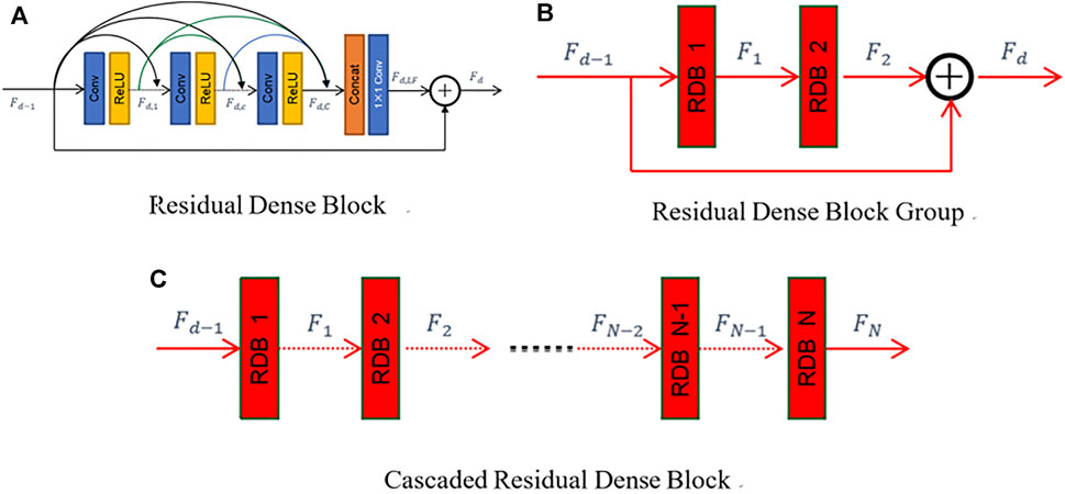
FIGURE 3. Comparison of RDB, CRDB, and RDBG. (A) RDB: it is a module with dense connections in the block. (B) RDBG (proposed method): it is composed of two RDBs. RDBG forms the LRD between blocks. (C) CRDB: the RDB is cascaded to form a network.

As shown in Figure 3C, Yang Aiping [16] et al. and X Liu [17] et al. used consecutive RDBs in a cascade manner. Since connections are also in blocks, in essence, it cannot fit LRD of images well.

Experimental Results and Discussions

The method proposed in this article will be compared with four state-of-the-art dehazing methods: DehazeNet, AOD-Net, DCP, and GFN.

Three metrics: PSNR, SSIM, and reference-less FADE are used to evaluate the quality of dehazing images. Our proposed method gets the best PSNR and SSIM among all methods (Table 2), which means that our method has the largest similarities between the original images and the dehazing images in both image gray levels and image structures. It also has satisfied results in FADE (Table 2; Figure 4), which means that our method is robust and stable in dehazing.

TABLE 2

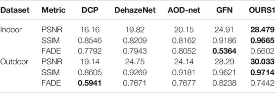
TABLE 2. PSNR, SSIM, and FADE between the dehazing results and original images of synthetic image in SOATS. The best results are marked by bold.

FIGURE 4

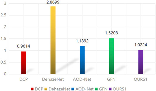
FIGURE 4. Average FADE of test results of different algorithms in real fog images collected in SOAT and the Internet.

The dehazing examples are given in Figures 5, 6, and their Hurst parameters are given under the foggy images.

FIGURE 5

FIGURE 5. Some dehazing images and their image quality metrics of synthetic foggy data in SOATS.

FIGURE 6

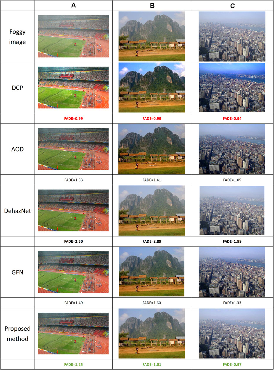
FIGURE 6. Some dehazing images and their image quality metrics of real foggy data in SOATS and on the Internet.

Conclusion

Assuming the foggy images are of fGn and calculating their Hurst parameters, the LRD of over 1,000 foggy images are proven by the fact that their Hurst parameters are all more than 0.6. Motivated by the LRD of foggy images, the Residual Dense Block Group (RDBG) with additional long skips between two RDBs is proposed. The RDBG utilizes information of LRD foggy images well and can obtain satisfied dehazing images.

Data Availability Statement

The original contributions presented in the study are included in the article/Supplementary Material; further inquiries can be directed to the corresponding authors.

Author Contributions

All authors listed have made a substantial, direct, and intellectual contribution to the work and approved it for publication.

Funding

The Chengdu Research Base of Giant Panda Breeding, Grant/Award Number: 2020CPB-C09, CPB2018-01, 2021CPB-B06, and 2021CPB-C01.

Conflict of Interest

The authors declare that the research was conducted in the absence of any commercial or financial relationships that could be construed as a potential conflict of interest.

Publisher’s Note

All claims expressed in this article are solely those of the authors and do not necessarily represent those of their affiliated organizations, or those of the publisher, the editors, and the reviewers. Any product that may be evaluated in this article, or claim that may be made by its manufacturer, is not guaranteed or endorsed by the publisher.

References

1. Cai B, Xu X, Jia K, Qing C, Tao D DehazeNet: An End-To-End System for Single Image Haze Removal. IEEE Trans Image Process (2016) 25(11):5187–98. doi:10.1109/tip.2016.2598681

PubMed Abstract | CrossRef Full Text | Google Scholar

2. Li B, Peng X, Wang Z, Xu J, Feng D. AOD-net: All-In-One Dehazing Network[C]. In: Proceeding of the 2017 IEEE International Conference on Computer Vision (ICCV); 22-29 Oct. 2017; Venice, Italy. IEEE (2017). p. 4780–8. doi:10.1109/iccv.2017.511

CrossRef Full Text | Google Scholar

3. Zhang H, Patel VM. Densely Connected Pyramid Dehazing Network[C]. In: Proceeding of the 2018 IEEE/CVF Conference on Computer Vision and Pattern Recognition (CVPR); 18-23 June 2018; Salt Lake City, UT, USA. IEEE (2018). p. 3194–203. doi:10.1109/CVPR.2018.00337

CrossRef Full Text | Google Scholar

4. Hochreiter S, Schmidhuber J Long Short-Term Memory. Neural Comput (1997) 9:1735–80. doi:10.1162/neco.1997.9.8.1735

PubMed Abstract | CrossRef Full Text | Google Scholar

5. Zaremba W, Sutskever I, Vinyals O. RECURRENT NEURAL NETWORK REGULARIZATION. In: International Conference on Learning Representations (ICLR) 2015; 2015 May 7–9; San Diego, CA (2014).

Google Scholar

6. Ren W, Ma L, Zhang J, Pan J, Cao X, Liu W, et al. Gated Fusion Network for Single Image Dehazing [J]. Proc IEEE Conf Computer Vis Pattern Recognition(CVPR) (2018), p. 3253–3261. doi:10.1109/CVPR.2018.00343

CrossRef Full Text | Google Scholar

7. Liao Z, Tang YY. Signal Denoising Using Wavelet and Block Hidden Markov Model. Int J Pattern Recognition Artif Intelligence (2005) 19(No. 5):681–700. doi:10.1142/s0218001405004265

CrossRef Full Text | Google Scholar

8. Li M Modified Multifractional Gaussian Noise and its Application. Physica Scripta (2021) 96(12):125002. doi:10.1088/1402-4896/ac1cf6

CrossRef Full Text | Google Scholar

9. Li M Generalized Fractional Gaussian Noise and its Application to Traffic Modeling. Physica A (2021) 579:1236137. doi:10.1016/j.physa.2021.126138

CrossRef Full Text | Google Scholar

10. Li M Multi-fractional Generalized Cauchy Process and its Application to Teletraffic. Physica A: Stat Mech its Appl (2020) 550:123982. doi:10.1016/j.physa.2019.123982

CrossRef Full Text | Google Scholar

11. He J, George C, Wu J, Li M, Leng J. Spatiotemporal BME Characterization and Mapping of Sea Surface Chlorophyll in Chesapeake Bay (USA) Using Auxiliary Sea Surface Temperature Data. Sci Total Environ (2021) 794:148670. doi:10.1016/j.scitotenv.2021

PubMed Abstract | CrossRef Full Text | Google Scholar

12. He J Application of Generalized Cauchy Process on Modeling the Long-Range Dependence and Self-Similarity of Sea Surface Chlorophyll Using 23 Years of Remote Sensing Data. Front Phys (2021) 9:750347. doi:10.3389/fphy.2021.750347

CrossRef Full Text | Google Scholar

13. Zhang Y, Tian Y, Kong Y, Zhong B, Fu Y. Residual Dense Network for Image Super-Resolution[J]. IEEE (2018).

Google Scholar

14. Li B, Ren W, Fu D, Tao D, Feng D, Zeng W, et al. Benchmarking Single Image Dehazing and Beyond[J]. IEEE Trans Image Process (2017) 28(1):492–505. doi:10.1109/TIP.2018.2867951

CrossRef Full Text | Google Scholar

15. Hurst HE Long-term Storage Capacity of Reservoirs. T Am Soc Civ Eng (1951) 116:770–99. doi:10.1061/taceat.0006518

CrossRef Full Text | Google Scholar

16. Yang A-P, Jin L, Jin-Jia X, Xiao-Xiao L, He Y-Q. Content Feature and Style Feature Fusion Network for Single Image Dehazing. ACTA Automatica Sinica (2021) 1–11. [2021-03-25]. doi:10.16383/j.aas.c200217

CrossRef Full Text | Google Scholar

17. Liu X, Ma Y, Shi Z, Chen J. GridDehazeNet: Attention-Based Multi-Scale Network for Image Dehazing [C]. In: Proceeding of the 2019 IEEE/CVF International Conference on Computer Vision (ICCV); Seoul, Korea; 2019 Oct 27–Nov 2. IEEE (2019), p. 7313–7322. doi:10.1109/ICCV.2019.00741

CrossRef Full Text | Google Scholar

18. Girshick R Fast R-CNN. In: IEEE International Conference on Computer Vision (ICCV); 2015 Dec 7–13; Santiago, Chile (2015). p. 1440–1448. doi:10.1109/ICCV.2015.169

CrossRef Full Text | Google Scholar

19. Johnson J, Alahi A, Fei-Fei L. Perceptual Losses for Real-Time Style Transfer and Super-Resolution[J]. Computer Sci (2016).

Google Scholar

20. Russakovsky O, Deng J, Su H, Krause J, Satheesh S, Ma S, et al. ImageNet Large Scale Visual Recognition Challenge. Int J Comput Vis (2015) 115(3):211–52. doi:10.1007/s11263-015-0816-y

CrossRef Full Text | Google Scholar

21. Simonyan K, Zisserman A. Very Deep Convolutional Networks for Large-Scale Image Recognition[J]. In International Conference on Learning Representations (ICLR); 2015 May 7–9; San Diego, CA (2014).

Google Scholar

22. Hu J, Shen L, Albanie S, Sun G, Wu E Squeeze-and-Excitation Networks[J]. IEEE Trans Pattern Anal Machine Intelligence (2017).

Google Scholar

23. Wang Z, Bovik AC, Sheikh HR, Simoncelli EP. Image Quality Assessment: from Error Visibility to Structural Similarity. IEEE Trans Image Process (2004) 13(4):600–12. doi:10.1109/tip.2003.819861

PubMed Abstract | CrossRef Full Text | Google Scholar

24. Choi LK, Jaehee You J, Bovik AC Referenceless Prediction of Perceptual Fog Density and Perceptual Image Defogging. IEEE Trans Image Process (2015) 24(11):3888–901. doi:10.1109/tip.2015.2456502

PubMed Abstract | CrossRef Full Text | Google Scholar

2020CPB-C09 CPB2018-02 CPB2018-01