
95% of researchers rate our articles as excellent or good
Learn more about the work of our research integrity team to safeguard the quality of each article we publish.
Find out more
ORIGINAL RESEARCH article
Front. Phys. , 18 November 2022
Sec. Cosmology
Volume 10 - 2022 | https://doi.org/10.3389/fphy.2022.823592
This article is part of the Research Topic Interaction Between Macroscopic Quantum Systems and Gravity View all 6 articles
 Nader A. Inan1,2,3*
There is much discrepancy in the literature concerning the possibility of a superconductor expelling gravito-electromagnetic fields just as it expels electromagnetic fields in the Meissner effect. Contradicting results are found in at least 18 papers written collectively by more than 20 authors and published over the course of more than 55 years (from 1966 to the present year of 2022). The primary purpose of this paper is to carefully explain the reason for the discrepancies, and provide a single conclusive treatment which may bring coherence to the subject. The analysis begins with a covariant Lagrangian for spinless charged particles (Cooper pairs) in the presence of electromagnetic fields in curved space-time. It is known that such a Lagrangian can lead to a vanishing Hamiltonian. Alternatively, it is shown that using a “space + time” Lagrangian leads to an associated Hamiltonian with a canonical momentum and minimal coupling rule. Discrepancies between Hamiltonians obtained by various authors are resolved. The canonical momentum leads to a modified form of the London equations and London gauge that includes the effects of gravity. A key result is that the gravito-magnetic field is expelled from a superconductor with a penetration depth on the order of the London penetration depth only when an appropriate magnetic field is also present. The gravitational flux quantum (fluxoid) in the body of a superconductor, and the quantized supercurrent in a superconducting ring, are also derived. Lastly, the case of a superconducting ring in the presence of a charged rotating mass cylinder is used as an example of applying the formalism developed.
Over the course of many decades, researchers have investigated a wide variety of new theoretical gravitational effects and the possibility of experiments that can detect these effects. Many of these include the use of superconductors [1–3], [11–27], [30–35], [38–47], [49, 50, 58, 59, 62], [63–66], [71–78], [80], [83–91], [100, 101, 104, 105], [109–111]. Some of the earliest interest in this topic is exhibited by the founding of the Gravity Research Foundation (GRF) in 1949 by Roger Babson. “His views were reflected by the wording in the announcement of the first essay competition that said the awards were to be given for suggestions for anti-gravity devices, for partial insulators, reflectors, or absorbers of gravity, or for some substance that can be rearranged by gravity to throw off heat - although not specifically mentioned in the announcement, he was thinking of absorbing or reflecting gravity waves.” [1]
Yet by 1953, the winning GRF essay by Bryce DeWitt dispensed with such endeavors as unrealizable. DeWitt expressed doubt that a material which absorbs or reflects gravity exists [2]. He states, “... first fix our sights on those grossly practical things, such as ‘gravity reflectors’ or ‘insulators,’ or magic ‘alloys’ which can change ‘gravity’ into heat, which one might hope to find as the usual by-products of new discoveries in the theory of gravitation... Of primary importance is the extreme weakness of gravitation coupling between material bodies ... The weakness of this coupling has the consequence that schemes for achieving gravitational insulation, via methods involving fanciful devices such as oscillation or conduction, would require masses of planetary magnitude.”
However, in 1966 DeWitt’s viewpoint apparently changed when he published a highly influential paper predicting the gravito-magnetic field (also known as frame-dragging or Lense-Thirring field) is expelled from superconductors in a Meissner effect [3]. It is evident DeWitt considered quantum mechanical systems (such as superconductors) may possess properties that were not previously considered when the statement was made barring the possibility of gravitational reflectors or insulators.
In [3], DeWitt begins with the Lagrangian for a relativistic spinless charged particle in an electromagnetic field in curved space-time and develops the associated Hamiltonian. He identifies a minimal coupling rule involving a gravitational vector potential and concludes this result implies the associated gravitational field must be expelled from a superconductor, just as the magnetic field is expelled from a superconductor in the Meissner effect.
DeWitt’s novelty and intuition is highly commendable, and his paper in [3] has been extremely influential in the field of gravity and superconductors. However, it will be shown that there may be some technical shortcomings in his treatment. Also, his interpretation of the flux quantization condition, and his order of magnitude calculation for an induced electric current, are questioned. In particular, the following items will be demonstrated.
• In [3], the Hamiltonian for a relativistic spinless charged particle in curved space-time is given by DeWitt as
where gμν is stated as the inverse metric, and
• In [3], the weak field, low velocity limit of the Hamiltonian is written as
where
Here e and m are the charge and mass of an electron, respectively. The appearance of
• The Hamiltonian in Eq. 2 implies a minimal coupling rule given by
• It is also stated in [3] that the flux of
• The gravito-magnetic field used in [3] is coordinate-dependent. With an appropriate coordinate transformation, the field can be made to vanish. Therefore, the corresponding gravitational Meissner-like effect is also coordinate-dependent and can be made to vanish as well. By contrast, a coordinate invariant formulation can be used which does not vanish by a coordinate transformation (to linear order in the perturbation).
• Lastly, it is claimed in [3] that a magnetic flux must arise in a superconducting ring that is concentric with a massive cylinder that begins rotating since it will produce a gravito-magnetic flux in the ring. It is predicted that the ring will remain in the n = 0 state, and an electric current will therefore be induced with an order-of-magnitude given by
where V is the rim speed, M is the mass, and d is the diameter of the rotating cylinder. However, it will be shown that the electric current predicted by Eq. 4 is actually limited to
Section 2 begins with a covariant Lagrangian for a relativistic spinless charged particle in an electromagnetic field in curved space-time. The Euler-Lagrange equation of motion leads to the geodesic equation of motion modified by the Lorentz four-force in curved space-time. Although the equation of motion correctly describes the dynamics of the particle, the associated Hamiltonian is identically zero and therefore cannot be used to describe a quantum mechanical system such as a superconductor.
Alternatively, a “space + time” Lagrangian is used to obtain a canonical three-momentum and Hamiltonian valid to all orders in the metric. The result is compared to DeWitt’s in Eq. 1. Some relevant metric relationships will be used to match the Hamiltonian with that of other authors for confirmation of its validity. The Hamiltonian is then expanded to first order in the metric to show the lowest order coupling of the momentum, electromagnetic fields, and gravity. Again, the result is compared to DeWitt’s result in Eq. 2. The Hamiltonian is further simplified by introducing the trace-reversed metric perturbation and assuming non-relativistic gravitational sources. Alternative Hamiltonians are also discussed as well as the conditions necessary for a Hamiltonian to be quantized.
In Section 3, gravito-electric and gravito-magnetic fields are defined in terms of the metric perturbation. Using the stress tensor of a non-relativistic ideal fluid, and the linearized Einstein field equation in harmonic coordinates, leads to gravito-electromagnetic field equations. In addition, the canonical momentum is used to develop constitutive equations for the supercurrent. These lead to a modified set of London equations describing the interaction of electromagnetic and gravito-electromagnetic fields with a superconductor. A modification to the London gauge condition is also identified.
In Section 4, the constitutive equations are used in the field equations to identify a penetration depth associated with the magnetic field and the gravito-magnetic field. It is found that the usual London penetration depth for the magnetic field is modified by the presence of a gravito-magnetic field, however, the modification is miniscule. It is also found that in the absence of a magnetic field, the superconductor demonstrates a paramagnetic effect rather than a diamagnetic (Meissner) effect for the gravito-magnetic field. In other words, the gravito-magnetic field is not expelled. However, when the magnetic field and the gravito-magnetic field are both present, it is possible for the gravito-magnetic field to be expelled with a penetration depth on the same order as the London penetration depth. However, it is demonstrated that the gravito-magnetic field is a coordinate-dependent quantity and therefore effects associated with it can be made to vanish with an appropriate coordinate transformation.
In Section 5, it is found that the usual London penetration depth for the electric field is modified by the presence of a gravito-magnetic field, however, again the modification is miniscule. In the process of developing these results, a penetration depth is also found for a field defined as the linear combination of the magnetic and gravito-magnetic vector potentials. However, since the gravito-magnetic vector potential is time-independent in this approximation, then it is shown not to have an associated penetration depth. This is expected since it is known that the Newtonian gravitational field generally cannot be shielded.
In Section 6, the new minimal coupling rule obtained in Section 2 will be used to write the Ginzburg-Landau supercurrent with coupling to electromagnetism and gravity. The complex order parameter must be single-valued around a closed path according to the Byers-Yang theorem. Then using the fact that all the fields vanish within the body of the superconductor leads a quantization condition for the flux of the magnetic and gravitational fields.
Lastly, in Section 7, the canonical momentum is used to develop an expression for the Ginzburg-Landau phase around a superconducting ring. Once again, using the fact that the wave function is single-valued around a closed path leads to a quantization condition involving the flux of the magnetic and gravitational fields, as well as the supercurrent around a superconducting ring. A charged, rotating mass cylinder is introduced as a source for electromagnetic and gravitational fields. The effect of placing the rotating cylinder coaxial with the superconducting ring is carefully analyzed. It is argued that the electric current predicted by DeWitt in Eq. 4 is not induced. Rather, the supercurrent in the ring is quantized along with the flux of electromagnetic and gravitational fields through the ring.
Using an action of the form
where uμ = dxμ/dτ is the four-velocity,
leads to the geodesic equation of motion modified by the Lorentz four-force in curved space-time
where
However, it is known that using Eq. 5 in a covariant Legendre transformation,
For the purposes of this paper, we will take an approach similar to [3, 11] by reparametrizing the action for the Lagrangian in Eq. 5 in terms of coordinate time rather than proper time.3 Note that the four-velocity can be written as uμ = γvμ, where the Lorentz factor is γ = dt/dτ, the coordinate velocity is
Therefore the action can be written as
This is the Lagrangian used by DeWitt [3] except he uses the notation
Then the canonical three-momentum, Pi = ∂L/∂vi, can be found from Eq. 11 to be
Note that pμ = gμνpν and
Therefore Eq. 13 can be written as simply pi = Pi − eAi which is consistent with the covariant canonical momentum relationship, pμ = Pμ − eAμ. Similarly, in [10] a covariant canonical momentum of the form Pμ = mgμνvν + qAμ appears. In [13], a canonical momentum is shown as Pi = mgijuj − eAi, where uj = γvj. This form is missing the term involving γmcg0i in Eq. 13 which may be because the canonical momentum in [13] is not formally derived from a Lagrangian but obtained by replacing the canonical momentum in flat space-time with a form proposed for curved space-time. Also [14, 15], have a result similar to Eq. 13 but without the terms involving A0 and Ai. This is due to starting from a Lagrangian similar to Eq. 11 but without the electromagnetic field.
Using gμν = ημν + hμν, where ημν is the Minkowski metric of flat space-time, and hμν is a perturbation, makes Eq. 13 become
In [16], a result similar to Eq. 15 is obtained but with h0i = 0 and γ = 1 due to using transverse-traceless coordinates
Note that in the absence of electromagnetism and gravity, the canonical momentum reduces to Pi = γmvi. Therefore, Eq. 15 implies that the presence of electromagnetism and gravity leads to a minimal coupling rule given by
For an electron
Using a Legendre transformation, H = Pkvk − L, requires solving Eq. 17 for vi which requires constructing the inverse of gik. This is shown in
which satisfies
Expressions equivalent to Eq. 19 can also be found in [11, 14, 15]. Inserting Eq. 19 into Eq. 17, and making use of Eq. 13 with q = −e, makes the Hamiltonian become
This can be considered a “space + time” Hamiltonian for a relativistic spinless charged particle in an electromagnetic field in curved space-time5. The result is exact in the metric perturbation and particle velocity. To compare with DeWitt’s result in Eq. 1, we can use Eq. 14 to write the Hamiltonian as
This matches DeWitt’s result in Eq. 1 except that DeWitt uses gjk instead of
In the literature, the “space + time” Hamiltonian appears in several other forms. To compare with Eq. 20, the following metric relationships developed in Supplementary Appendix SA can be used:
Using Eq. 22 in Eq. 20 leads to a form that matches Cognola, Vanzo, and Zerbini [11].
It is stated in [11] that Eq. 23 and DeWitt’s result in Eq. 1 are not equivalent when there is a nonvanishing g0i. However, it is demonstrated here that Eq. 20, which is the corrected form of DeWitt’s approach, is indeed equivalent to Eq. 23 via the use of Eq. 22. Also, substituting Eq. 18 into Eq. 23 leads to a result that matches Bertschinger [9], except [9] does not include electromagnetic fields.
With some algebraic manipulation, this Hamiltonian also matches the result derived by Piyakis, Papini, and Rystephanick [32].
Therefore, the discrepancies between all of the authors stated above are resolved.
The lowest order expansion of Eq. 20 is now considered. As discussed below Eq. 7, the canonical four-momentum is found to be Pμ = pμ + eAμ. Using the metric perturbation leads to
This shows that to lowest order,
Following the procedure of Supplementary Appendix SB, but remaining to first order in the perturbation and second order in momentum, leads to
To compare with DeWitt’s result in Eq. 2, the indices of the electromagnetic potentials can be lowered using Eq. 14. Remaining to first order in the perturbation leads to
Although Eq. 28 has the benefit of being more compact than Eq. 27, it can be misleading due to the fact that Ai and A0 contain metric perturbation terms as demonstrated by Eq. 14. In fact, terms that are second order in
The following are comparisons between DeWitt’s result in Eq. 2 and the result obtained in Eq. 28.
• The Hamiltonian in Eq. 28 contains the scalar, vector, and tensor parts of the metric perturbation which are, respectively, h00, h0i, and hij. The tensor part of the perturbation is still first order in the perturbation6 but is missing in Eq. 2. In fact, all the terms after ecA0 in Eq. 28 are missing from Eq. 2. It is shown in Supplementary Appendix SB that the terms involving
• The expression appearing as
• The expression appearing as
• The Hamiltonian in Eq. 2 implies a minimal coupling rule given by
The Hamiltonian in Eq. 31 can also be written using the trace-reversed metric perturbation,
A gravito-scalar potential and gravito-vector potential can also be defined as, respectively,
For brevity, a minimally coupled canonical momentum can be defined as
Terms are listed from largest to smallest magnitude based on the order-of-magnitude analysis found in Supplementary Appendix SB. Terms within an order of magnitude are grouped in parentheses. It is shown that using the maximum momentum permitted for Cooper pairs (which requires keeping the kinetic energy below the BCS energy gap), and estimating the largest value for hi that can be reasonably produced in a lab, then hiPi ∼ 10–47 J while
where A2 = AiAi. Note that the terms involving
Again, terms are listed from largest to smallest magnitude. Notice the term involving
The following is a discussion of the various covariant Hamiltonians that describe the same particle dynamics, and the differing ways that a “space + time” Hamiltonian has been derived by various authors. It is emphasized that all of these approaches found throughout the literature are shown here to be equivalent. The issue of a vanishing covariant Hamiltonian, and the issue of singular Lagrangians is also discussed.
It was stated after Eq. 7 that using a Lagrangian,
However, it is demonstrated in [51] that even L1 is singular due to the constraint uμuμ = −c2. It is also shown in this paper that the Hamiltonians in Eq. 20 and Eq. 23 are equivalent. Therefore, contrary to the statement in [11], it is demonstrated here that both Eq. 20 and Eq. 23 are valid expressions of the “space + time” Hamiltonian despite the fact that they are both derived from a singular Lagrangian, L1.
Furthermore [9], shows that a covariant Lagrangian of the form
As an extension to this approach, it was shown in [12] that electromagnetic fields can also be included by writing
This topic is also discussed in [8] where two covariant Hamiltonians are shown. One of them is
Lastly, note that the method used in this paper to obtain the “space + time” Hamiltonian in Eq. 20 is different from the method used by [12] to obtain the “space + time” Hamiltonian in Eq. 23. In this paper,
Concerning the quantization of a classical Hamiltonian, it is common to simply promote canonical quantities to quantum operators. Then xi and Pj are replaced with
In [8], it is shown that the general theory of canonical transformations and Poisson brackets in Hamilton-Jacobi theory can be put in covariant form for a single particle. However, it is noted that a relativistic theory of multiple interacting particles introduces the complication that we cannot assume a common proper time for all particles.
In the case of Eq. 32, the issue of proper time is avoided by using a “space + time” approach, as well as the Lorentz factor obtained in Eq. 19. The Lorentz factor essentially removes proper time in favor of coordinate time and the metric. Therefore, Eq. 32 can be generalized to a collection of particles which are assumed to be embedded in the same space-time metric, with velocities measured by an observer in terms of a single coordinate time. This is particularly relevant to the fact that DeWitt states in [3], “For the Hamiltonian of the ensemble of free electrons inside a superconductor, Eq. 2 is replaced by
where
In [8], it is also pointed out that using
Lastly, a modified Schrödinger equation can be obtained from Eq. 33. Dropping the rest mass energy and acting the Hamiltonian on a wave function,
In the absence of gravity, this reduces to the usual Schrödinger equation in the presence of an electromagnetic field. In that case, the solution could be written as
similar to what is shown in [14, 15, 30, 35, 40, 42, 44, 47]. However, this is not how the presence of gravity appears in Eq. 35. Rather, gravity enters as a multiplicative factor to a first derivative term, hi∂i, not an additive factor inside the second derivative term. In fact, attempting to use ψ = eiϕψ0, with a phase given by Eq. 36, leads to
This topic can be understood in the context of a covariant Ginzburg-Landau model [50, 57–63]. The transformations of a complex scalar field and the four-potential can be written, respectively, as
In curved space-time, the gauge covariant derivative becomes
In fact, since the gauge covariant derivative transforms as
A possible cause for confusion is the fact that quantizing the canonical momentum Eq. 16 leads to
This seems to imply that
In fact, since Eq. 35 involves a second order spatial derivative, then this issue can be further understood by starting from a second order covariant derivative acting on a scalar wave function in the absence of electromagnetic fields: gμν∇μ∇νψ. Since ψ is a scalar, then the first covariant derivative of ψ is just a partial derivative: ∇νψ = ∂νψ. However, since ∂νψ is a vector, then acting the second covariant derivative brings in the Christoffel symbol:
Similar to Eq. 35, it is found that h0i multiplies a first derivative term, rather than appearing as an additive factor inside the second derivative term. Furthermore, Eq. 38 can be used to write the Klein-Gordon equation in curved space-time as
Again, notice that h0i is multiplying
In summary, the distinction between the way gravity and electromagnetism couple to a quantum field is fundamentally the reason for the difference in the way they appear in the modified Schrödinger equation Eq. 35, and the reason why it is not the case that ψ = eiϕψ0, where ψ0 is the solution to the field-free Schrödinger equation if the phase is assumed to be Eq. 36. However, it will be shown in Sections 6, 7 that the canonical momentum Eq. 13 can be used to obtain a quantum phase with terms that include those appearing in Eq. 36.
On a more fundamental level,
However, the relative motion between a particle and an observer is uniquely described by the geodesic deviation equation. Therefore, it is argued in [77, 78] that a Hamiltonian based on the geodesic deviation equation is preferred (which involves the Riemann curvature tensor) versus a Hamiltonian based on the geodesic equation (which involves the Christoffel symbols). A similar approach was used by Weber15 in the context of gravitational wave detection [79].
In fact, it is shown in [78] that for the case of gravitational waves (in the weak field, low velocity limit), the Lagrangian leading to the geodesic deviation equation is
Another approach is the use of Fermi normal coordinates17 which also expresses the Hamiltonian in terms of the Riemann curvature tensor (which is coordinate invariant) rather than Christoffel symbols (which are coordinate dependent) [16, 34], [83–86]. There are also other approaches that depart entirely from the use of a Lagrangian associated with either the geodesic equation of motion or the geodesic deviation equation. For example [87], uses a Ginzburg-Landau free energy density that includes a coupling to gravity via a term involving the Ricci scalar.
On the other hand [88], uses a Hamiltonian derived from an effective field theory describing a system of quantum oscillators coupled to a stochastic gravitational radiation background, where the coupling to gravity occurs via a parameter associated with an Ohmic bath spectral density. Although [88] does not consider a superconductor, it is possible that a similar treatment could be used to describe the coupling of the stochastic gravitational wave background to a superconductor. Fundamentally, the coupling of the quantum system to gravity is obtained via the action for a scalar field stress tensor coupled to the curved space-time background [89].
On a related note, it should be emphasized that the action in Eq. 8 only describes the particle dynamics but treats electromagnetism and gravity as fixed background fields with no dynamics. This means that any fields produced by the motion of test particles (which are Cooper pairs leading to a supercurrent) are neglected. However, in Section 4 it is evident that the supercurrent does indeed produce fields which can lead to a Meissner effect. Therefore, a complete action should also include the dynamics of the fields by including terms for electromagnetism and gravity which are, respectively,
It is also shown in [10] that a Ginzburg-Landau Lagrangian density in curved space-time can be used to obtain a quantum current density and quantum stress tensor. The action has the form
In this section, gravito-electromagnetic field equations are introduced, and constitutive equations are developed from the canonical momentum and combined with the field equations to obtain a modified form of the London equations [94–96]. Using harmonic coordinates,
where ρM is mass density, and Vi is the velocity, of the gravitational sources. Note that in the presence of electromagnetic fields, the full stress tensor should also include
where the components of the electromagnetic strength tensor are
To lowest order, using E = cB, the components of Eq. 41 are
Comparing Eq. 43 to Eq. 40, it is evident that the contribution of electromagnetic fields to the total stress tensor can be neglected provided B2/μ0 ≪ ρMcV. For a superconductor such as niobium, we can use ρM ∼ 104 kg/m3. It is also shown in Supplementary Appendix SB that a maximum of v ∼ 104 m/s will preserve the superconducting state18. This leads to B ≪ 105 T which is certainly satisfied in a laboratory setting.
Since Tij ≈ 0, then
Defining the mass current density as
where
To develop constitutive equations for a superconductor, we begin by promoting the canonical momentum in Eq. 13 to a quantum mechanical operator,
This can be considered a semiclassical approach where the gravitational field, hμν, is still a classical field while
Applying Ehrenfest’s theorem allows this equation to return to a classical equation of motion once again. To first order in the metric perturbation, and first order in test mass velocity, Eq. 12 becomes γ ≈ 1 + h00/2 + h0jvj/c. Then using Eq. 29 and Eq. 30 in Eq. 47, remaining to first order in the metric perturbation, and using q = −e and m = me for electrons, leads to
A similar expression appears in [19] but the scalar potentials, φ and φG, are absent. The charge and mass supercurrent densities are, respectively20
where ns is the number density of Cooper pairs. Inserting Eq. 48 into Eq. 49
and
where ΛL ≡ nse2/me can be defined as the London constant, and
The expressions in Eq. 50 and Eq. 51 are the London constitutive equations for a non-relativistic supercurrent in the presence of electromagnetism and gravity (from non-relativistic gravitational sources in harmonic coordinates). Similar expressions can be found in [22–24], [26], however, with α = 1 and β = me/e which is a special case where φG = 0 and φ = 0. Notice that if
and
Equations similar to Eq. 53 and Eq. 54 are also obtained in [17, 21, 22, 24, 71, 72], but with the absence of the gravitational and electric scalar potentials which means α = 1,
Taking the curl of Eq. 50 and Eq. 51, and using Eq. 44, leads to, respectively,
and
Similar expressions can be found in [17, 20, 71, 72], however, with α = 1 and β = me/e. Notice that Eq. 55 is the usual magnetic London equation,
The same result is obtained in [26, 27, 62, 73, 100]. A result similar to Eq. 57 is also obtained in [74, 75], however, it will be shown later that there is a critical sign difference which impacts whether a gravito-magnetic Meissner effect is predicted to occur in the absence of a magnetic field.
Concerning the gauge condition, note that the usual London gauge,
This is the modified gauge condition associated with the London equations developed above. It is similar to the gauge condition shown in [74, 75] as
Lastly, taking the curl of Eq. 55, using
It will be shown in the following section that αμ0ΛL ≫ βμGnse and α ≈ 1. Also, using
where the London penetration depth is
Notice that Eq. 59 contains a quantity which can be defined as
As explained in the following section, this quantity can be understood as leading to a modified London penetration depth,
The Maxwell equation (with sources) in curved space-time is
where
Since
Then Eq. 63 becomes
Setting μ = i, and using Eq. 30, Eq. 44, and Eq. 42 leads to
This is the usual Ampere law but with added corrections due to the presence of gravity.
Assume a steady-state supercurrent so that
Since
where
Notice that α′ differs from α in Eq. 52 by an additional factor given by
A similar treatment can be applied to the gravito-Ampere law in Eq. 45 which is
Coupled differential equations similar to Eq. 69 and Eq. 71 can also be found in [18–22]. In the absence of gravity, α = 1 and
where
For a superconducting slab occupying the region z > 0, where z is the distance from the surface to the interior of the superconductor, then the boundary conditions for the magnetic field are
where
Three other cases are now considered which involve gravity:
1. The presence of only
2. The effect of
3. The effect of
If
In fact, for a maximum gravito-magnetic field at the surface of the superconductor
Note that Eq. 74 can also be written in the following alternative forms using μ G = 4πG/c 2 and Eq. 61.
To obtain a numerical estimate for this quantity, consider a superconductor such as niobium which has a London penetration depth of λ L ∼ 10−9 m. Then Eq. 75 gives approximately 1022 λ L ∼ 1013 m which is clearly not observable on a terrestrial scale.
The absence of a gravito-magnetic Meissner effect (when
However, in the case of [19], the issue is more subtle. The gravito-vector potential is defined as
In the case of [74, 75], the gravito-vector potential is defined as
In the case of [26, 27], the presence of a gravito-magnetic Meissner effect is argued on the basis of spontaneous symmetry breaking. A Lagrangian is written in the form
In the case of [73], there is discussion about whether the “covariant derivative” is
For a charged supercurrent in the presence of both magnetic and gravito-magnetic fields, the differential equations Eq. 69 and Eq. 71 need to be decoupled to obtain solutions. For simplicity, consider a system arranged such that
where k matches Eq. 62 which is
The modified London penetration depth can be defined as
Notice that the first term in Eq. 78 encodes a correction due to the gravitational scalar potential, while the second term encodes a correction due to the electric scalar potential. An order of magnitude can be calculated for each term in Eq. 78 using Eq. 52. The first term on the right side of Eq. 78 implies a correction to the London penetration depth given by
For the second term in Eq. 78, note that if m
e
c
2 ≫ eφ, then β ≈ 4m
e
/e ∼ 10−11 kg/C. Also using n
s
∼ 1026 m−3 means the second term in Eq. 78 is
Since
Using the boundary conditions in Eq. 73 leads to
This is the standard Meissner effect but with a modified London penetration depth given by Eq. 78. Notice that the first term in Eq. 78 encodes a correction due to the gravitational scalar potential since α = 1 + φ
G
/c
2. The second term in Eq. 78 encodes a correction due to the gravito-magnetic field since it can be traced back to the terms involving
Again, for simplicity, consider a system arranged such that
where k is given by Eq. 77. For a neutral superfluid (or in the absence of a magnetic field), Eq. 77 reduces to k
2 = −4μ
G
n
s
m
e
and therefore Eq. 81 leads to a paramagnetic effect, as stated before. However, for a charged supercurrent in the presence of both
The general form of the solutions in Eq. 79 and Eq. 82 are also found in [20]. Using the boundary conditions in Eq. 73 leads to
This result predicts a diamagnetic (Meissner) effect for the gravito-magnetic field when a magnetic field is also present. In fact, the gravito-magnetic field is expelled with approximately the same penetration depth as the magnetic field. Defining the gravitational penetration depth as λ G ≡ 1/k, and using Eq. 77 gives
Therefore, it is found that
This effect can be understood by comparing how the physics contained in Eq. 77 applies to the magnetic field versus the gravito-magnetic field. As it applies to the magnetic field, Eq. 77 predicts a diamagnetic (Meissner) effect with only a miniscule modification due to the presence of the gravito-magnetic field. However, as it applies to the gravito-magnetic field, Eq. 77 predicts a paramagnetic effect which is drastically altered by the presence of the magnetic field. In fact, the alteration is so substantial that it switches a paramagnetic effect into a diamagnetic (Meissner) effect for the gravito-magnetic field.
This can be further understood by returning to Eq. 71 and noticing that when
This description also demonstrates that there is a threshold value for the minimum magnetic field necessary to produce a Meissner effect for the gravito-magnetic field. It is given by
Hence the findings above are summarized as follows:
• A supercurrent in the presence of only
• A supercurrent in the presence of only
• A supercurrent in the presence of both
• A neutral superfluid in the presence of
These results demonstrate an important interaction between electromagnetism, gravitation, and a quantum mechanical system that only occurs when all three are present. The superconductor provides the quantum mechanical system which is necessary to have any kind of Meissner effect. The gravito-magnetic field is required to create a novel gravitational effect. Lastly, the magnetic field is necessary to mediate the interaction. In the absence of a magnetic field, the novel gravito-magnetic Meissner effect would not take place.
Note that the conclusion that both
Using Eq. 60 and
where σ
c,0 ≡ λ
L
J
c,0 and σ
m,0 ≡ λ
L
J
m,0 are charge and mass surface current densities, respectively. Similarly, the solutions for
The use of Eq. 86 leads to solutions for
The following observations can be made about Eq. 87.
• It is noted in [20–22] that
• It is also noted in [20] that the absence of an external magnetic field,
The first expression is consistent with the absence of a gravito-magnetic Meissner effect when there is no magnetic field. The second expression means that a gravito-magnetic field will generate a very small magnetic field in the interior of the superconductor.
• It is noted in [21] that the absence of an external gravito-magnetic field,
The first expression can be understood as a result of the magnetic field generating screening currents which produce a gravito-magnetic field. Therefore,
• The expressions in Eq. 89 both involve μ g /μ. Based on this, it is stated in [22] that the material properties of the superconductor will determine the residual fields which could lead to experimentally observable gravitational effects.
• Lastly, the residual fields in Eq. 87 can be interpreted as expressions associated with
Notice there are residual terms remaining when z ≫ λ
L
. However, setting B
0 = μ
0
σ
c,0 leads to the usual solution,
In the case of [71, 72], a “generalized field” is defined as
where λ
e
is the London penetration depth, and λ
g
is essentially the expression found in Eq. 75. It is recognized that Eq. 91 becomes a Yukawa-like equation when λ
g
> λ
e
which leads to a “generalized Meissner effect.” Since λ
g
∼ 1013 m and λ
e
∼ 10−8 m, then the condition for a “generalized Meissner effect” is clearly satisfied. In fact, since λ
g
≫ λ
e
, then and the “generalized penetration depth” from Eq. 91 becomes
In [74, 75], the same approach is used except the combined field is defined as
A final important consideration is the issue of coordinate-freedom in linearized General Relativity. The gravito-magnetic field,
Therefore, the effects associated with
Using
On the left side of both equations, we can use the identity
and
Since
In the case of [20, 24], the gravitational sources are non-relativistic
In the case of [71–73], the exact same problem is at the root of the analysis. Again the gravitational sources are non-relativistic
Returning to Eq. 94, an expression for the electric field can be obtained by taking a time derivative and using
In the absence of gravity, Eq. 96 becomes
However, if φ
G
and φ are time-dependent, then Eq. 96 requires obtaining solutions for
Multiplying Eq. 95 by β/α, adding the result to Eq. 98, and using a field defined as
where k is given by Eq. 77. Consider a system where
Taking a time derivative gives
Inserting Eq. 101 into Eq. 96 gives
where
where
In Ginzburg-Landau theory, the minimal coupling rule,
where
Staying to first order in the metric perturbation, and first order in test mass velocity, requires using γ ≈ 1 in Eq. 105. For convenience, the entire coupling vector can be defined as
Then the corresponding supercurrent becomes
which reduces to Eq. 104 in the absence of gravity. Using
An expression similar to Eq. 108 is found in [18, 19, 21, 23, 24, 26, 49], [71–75], [104, 105], however, the terms involving φ and φ G in Eq. 106 are missing. In the previous section, it was shown that inside the body of the superconductor (much deeper than the London penetration depth), all the fields in Eq. 48 vanish and therefore the supercurrent velocity is zero. Therefore, using J i = 0 in Eq. 108 and v i = 0 in Eq. 106 makes Eq. 108 become
Integrating around a closed loop gives
Since the order parameter is single-valued, then it must return to the same value when the line integral returns to the same point. Therefore, the right side must be 2πn, where n is an integer. 27
Applying Stokes’ theorem on the left side gives
where S is the surface bounded by the curve C. Using ∇φ = 0 within the body of the superconductor, and q = −2e and m = 2m e for Cooper pairs, gives
where Φ
B
and
In the absence of electromagnetism, the gravito-magnetic flux condition can be written as
In the absence of gravity, Eq. 113 gives the usual magnetic flux condition, Φ
B
= nΦ
B,0, where
where r = r 0 is the radius of a fluxoid. Then Eq. 113 in the n = 1 state can be written as
where S
0 is the area of a single fluxoid. Since the dominant source of
Since
The two terms involving gravity are small corrections. Therefore, solving for Φ B and keeping only lowest order terms involving E G and B G leads to
This result can be interpreted as a modified magnetic fluxoid in the presence of gravity. Since [107] used r
0 ∼ 10−5 m, then Eq. 114 gives A
0 ∼ 10−30 T⋅m. Therefore, the last term in Eq. 118 becomes
For the term involving
Promoting the canonical momentum in Eq. 13 to a quantum mechanical operator and acting on the complex order parameter gives
Again use Ψ = ψe
iϕ
, but now let
Applying Ehrenfest’s theorem allows this equation to return to a classical equation. Staying to first order in the metric perturbation and test mass velocity, and using Eq. 29 and Eq. 30 leads to
This expression can be written in terms of the supercurrent density, J i = −qn s v i . Then integrating around a closed loop gives
Since the order parameter is single-valued, then it must return to the same value when the line integral returns to the same point. Therefore, the right side must be 2πn, where n is an integer. Applying Stokes’ theorem on the left side, and using q = −2e and m = 2m e for Cooper pairs, gives
Since φ G ≪ c 2 and eφ ≪ m e c 2, then the expression can be approximated to
This result is similar to Eq. 113 which applies to the bulk of the superconductor. However, Eq. 124 contains additional terms involving
As a practical example, consider a superconducting ring in the presence of a rotating massive cylinder of length ℓ and radius R. The cylinder rotates at a constant non-relativistic angular velocity and hence has a stationary mass current (See Figure 1).
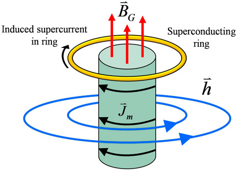
FIGURE 1. A rotating massive cylinder carries a mass current,
This is effectively the same system that was considered by DeWitt [3]. He states, “Now consider an experiment in which the superconductor is a uniform circular ring surrounding a concentric, axially symmetric, quasirigid mass. Suppose the mass, initially at rest, is set in motion until a constant final angular velocity is reached. This produces a Lense-Thirring field which, in a coordinate system for which the metric is time-independent, takes the form
where κ is the gravitation constant, and ρ and
Neglecting terms that are
DeWitt states, “If
A similar statement is found in Papini’s paper [111] which is a follow up to DeWitt’s paper [3]. Papini states, “The main result of this [DeWitt’s] work is that whenever a Lense-Thirring field is present, it is not the magnetic field which vanishes inside a superconductor, but a combination of magnetic and gravitational fields. Similarly, the flux which is quantized is the total flux of magnetic and gravitational fields... It is important that initially the total flux linking the loop be zero. The total flux is in fact quantized in units of π and if it vanishes in the initial state, it also vanishes in the final state. It then follows that the magnetic flux equals in absolute value the flux of the gravitational field.” Using Eq. 124, this condition can be written as
DeWitt states, “Suppose the rotating mass is kept electromagnetically neutral... Then the magnetic field must arise from a current induced in the ring. The magnitude of this current will be
where S is the area spanned by the ring, L is its self-inductance, and the final integral is taken around the ring.” Since a static flux does not generate a current, and the presence of inductance in Eq. 128 implies a changing current, then Faraday’s law and Eq. 127 must have been used to obtain
Integrating with respect to time gives
Evidently DeWitt assumes
except he sets c = 1. However, a more accurate estimate for Eq. 128 can be obtained using the gravito-magnetic flux evaluated in Supplementary Appendix SB as
where
The following objections can be raised concerning DeWitt’s treatment summarized above.
• The expression in Eq. 127 was obtained using an initial state with every term in Eq. 126 set to zero, then letting
• When
• Since a static flux does not generate a current, then Eq. 129 must be used to obtain an induced current. However, it was also stated that Eq. 125 was obtained “in a coordinate system for which the metric is time-independent.” Since the right side of Eq. 129 is zero for a time-independent metric, then no electric current would be predicted.
With these considerations in mind, it is suggested that a correct interpretation of Eq. 126 would be described as follows. Introducing a non-zero B
G
can generate a mass current in the ring via a gravito-Faraday flux rule. Because the mass current consists of Cooper pairs, then there will be an associated electric current,
In this sense, Eq. 126 plays the role of a constraint equation describing the quantization of the current, rather than a field equation that can generate a flux. To elaborate on this, we can return to the more general expression Eq. 124 and write it as
where the total flux through the ring is
If the current density is assumed to be uniform and only occupies the skin of the superconducting ring (no deeper than the penetration depth), then
where
is an “electric current quantum” analogous to the magnetic flux quantum,
Here the relative electric permittivity and magnetic permeability of the massive cylinder are, respectively, ɛ
r
= ɛ/ɛ
0 and μ
r
= μ/μ
0. Also d is the diameter of the ring. Notice from Eq. 138 that F is a continuous function of ω, however, the entire left side of Eq. 136 is discretized and can only increase by increments of I
0. This means that even though F can change gradually, the smallest change in F that can change the state of the system is ΔF = μ
0
eI
0
d/2, and each change by ΔF will move the system between n states. (If F changes by an amount smaller than μ
0
eI
0
d/2, the quantum “rigidity” of the Cooper pair wave function will preserve the state of the system.) However, since
For simplicity, consider if the diameter of the ring is similar to the diameter of the solenoid
and Eq. 136 becomes
This is the quantization condition for the superconducting ring in the configuration of Figure 1. Again, it is emphasized that we cannot set n = 0 and claim that
is generated in the ring. Rather, Eq. 141 should be interpreted as simply the smallest non-zero current that can exist in the ring. However, next we proceed to calculate the current that will be generated.
The current generated in the superconducting ring can be evaluated by developing a gravitational version of the Faraday flux rule. In Supplementary Appendix SD it is shown that the Lorentz four-force in curved space-time Eq. 7 can be evaluated to first order in the perturbation and test mass velocity to obtain
where the electromagnetic force is
the gravitational force is
and the electromagnetic force coupled to gravity is
The electromagnetic emf is given by
which leads to the usual Faraday flux rule,
where
which leads to an associated “gravitational Faraday flux rule” given by
where the notation “constant B G ” indicates that the term in parentheses involves a time-varying boundary, not a time-varying B G (which is accounted for in the next term). The emf generated by a time-varying boundary can be referred to as a motional gravitational emf, while the emf generated by a time-varying B G can be referred to as a transformer gravitational emf. Lastly, a “coupled emf” associated with Eq. 145 can be defined as
which becomes
The total emf associated with the total force Eq. 142 is
For the system in Figure 1, there is no electric field. Also, the gravito-scalar potential is primarily due to earth, therefore
Since φ
G
is primarily due to earth, then 1 − 3φ
G
/c
2 ≈ 1 − 10−9 ∼ 1. For simplicity, again we can approximate
where r is the time-varying radius of the ring. Consider if the ring is expanding at a constant rate, r = v b t, and define
where a characterizes electromagnetic effects, and b characterizes gravitational effects. Then Eq. 154 becomes
In the absence of gravity
which is indicative of the fact that gravity has a miniscule effect on the induced changes in the current. In superconductors, L ∼ 10−10 H at most [112]. Also, if v
b
∼ 1 m/s, then a ∼ 104 s−2. Therefore, 1 + 2at
2 ≈ 1 for
Note that the values of L and v b are not relevant until t ≪ 10−2 s is no longer satisfied.
As previously stated, Eq. 129 implies DeWitt was considering a situation associated with a transformer emf (not a motional emf) since he states, “Suppose the mass, initially at rest, is set in motion until a constant final angular velocity is reached.” It has been emphasized throughout this paper that the use of non-relativistic gravitational sources and harmonic coordinates leads to
However, to treat the system DeWitt was considering, we can relax this requirement and permit
where the notation “constant boundary” indicates that the term in parentheses involves a time-varying B G , not a time-varying boundary. Again, 1 − 3φ G /c 2 ∼ 1. This leads to a result similar to Eq. 154 but this time r = R (which is constant) but ω varies with time. Therefore we have
where
leads to
Again a′ characterizes electromagnetic effects, and b′ characterizes gravitational effects. Letting I = 0 at t = 0, and t = T when the mass cylinder reaches ω max, leads to the following solution to Eq. 162.
If α is constant, then ω max = αT. For the case of a large flywheel, again we can use M ∼ 4 × 10³ kg, R ∼ ℓ ∼ 1 m, and ω max ∼ 6 × 10² rad/s. Since L ∼ 10–10 H at most in superconductors [112], then 1 + a′ ≈ a′ ∼ 104 and Eq. 163 becomes
Note that the electric current produced by a motional gravitational emf Eq. 157 and transformer gravitational emf Eq. 164 are not unique to a superconductor since the London equations were not utilized anywhere in the analysis. The only feature in the calculation unique to superconductors is the value of the inductance, however, the inductance cancels in both calculations.
Alternatively, a treatment involving the London equations could begin with Eq. 53. When we permit
where we set
Applying this to the ring and using Eq. 132 leads to a magnitude given by
where
As previously stated, the effect of Eqs 167, 168 are in opposite directions. Therefore, using Eq. 165 as well as
This has the same form as Eq. 162 and therefore has a solution similar to Eq. 163.
Assuming α is constant, and using the same parameters for a large flywheel again leads to
Again, the result is not dependent on the inductance, and the value is comparable to Eq. 164. It is arguable that the result obtained in Eq. 171 is more reliable since it is calculated using the London equation which is derived from the canonical momentum. Therefore, it stems from a quantum mechanical approach (since the canonical momentum operator acting on the Ginzburg-Landau order parameter leads to the London equations). In contrast, Eq. 171 is derived from a purely classical equation of motion (the geodesic equation of motion with a Lorentz four-force). 32
Due to the current in the ring and the presence of magnetic and gravito-magnetic fields, there will be a corresponding Hall effect as shown in Figure 2.
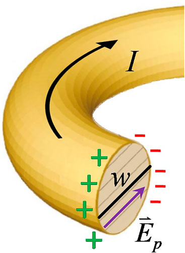
FIGURE 2. A polarization electric field,
Following the usual derivation of the Hall effect, we begin with the total force on the charge carriers. As previously stated,
where v
s
is the velocity of the supercurrent around the ring, and
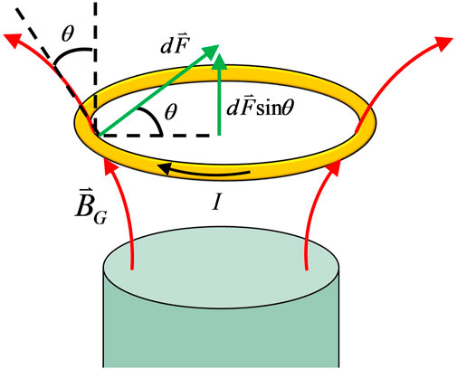
FIGURE 3. A superconducting ring placed above a rotating mass cyldiner. At the location of the ring,
The net effect of the magnetic and gravito-magnetic forces is to cause Cooper pairs to accumulate on the inner perimeter of the ring. As a result, there will be an electric field pointing radially inward. There will not be any
Following the usual derivation of the Hall effect, the total radial force on the charge carriers will be zero for a steady-state current. Also using
Then approximating 1 − 3φ G /c 2 ∼ 1 makes Eq. 173 become
We can approximate
The first term is purely electromagnetic and quadratic in the current, while the second term involves gravitational effects and is linear in the current. In fact, for the case of a large flywheel (M ∼ 4 × 10³ kg, R ∼ ℓ ∼ 1 m, ω ∼ 6 × 10² rad/s), the two terms become comparable when
This is similar to the result obtained in Eq. 157. Using Eq. 177 and ω ∼ 10−4 m in Eq. 176 gives
A gravitational Hall effect for a superfluid is also considered in [27], however, no Hall potential value is obtained.
Lastly, consider if the ring is raised some distance above the massive cylinder so that
A vertical force on the ring will exist due to the current in the ring and the gravito-magnetic field of the mass cylinder. This effect is analogous to the “jumping ring” experiment where a magnetic force is evaluated using
where
Recall that the differential magnetic force in a current segment,
In Supplementary Appendix SB, the gravito-magnetic field along the axis of the mass cylinder is found as
Approximating θ ≈ 300, using the case of a large flywheel (M ∼ 4 × 10³ kg, R ∼ ℓ ∼ 1 m, ω ∼ 6 × 10² rad/s), and I ∼ 10−26 A obtained in Eq. 171 leads to F ∼ 10−57 N which is completely negligible. To get a more substantial effect, an electric current can be driven in the ring prior to introducing B G from the massive cylinder. It is shown in Supplementary Appendix SB that the maximum supercurrent velocity that preserves the superconducting state is v ∼ 104 m/s. Then using Eq. 174 leads to
This is a factor of 1025 larger than the current induced by B G . Furthermore, it was previously mentioned that in a low Earth orbit (LEO) satellite, the gravito-vector potential due to earth (as observed by the satellite) is h LEO ∼ 10−3 m/s. Compared to the large flywheel (h ∼ 10−21 m/s) this leads to another factor of 1018 increase for B G . As a result, the force on a ring could be F ∼ 10−14 N.
On a related note, the factor of 1018 increase in
Since the gravito-vector potential of the earth cannot be controlled (unlike that of a spinning flywheel), an option for controlling the exposure of the system to
The following are key results demonstrated uniquely in this paper.
• The canonical momentum for a relativistic spinless charged particle in curved space-time is obtained in Eq. 13 as
where the Lorentz factor in curved space-time is
• A corrected version of DeWitt’s Hamiltonian Eq. 1 is given by the “space + time” Hamiltonian shown in Eq. 20 as
where
• The Hamiltonian that is first order in the metric perturbation and second order in momentum is found in Eq. 28 to be
The last three terms in Eq. 185 are missing from DeWitt’s result in Eq. 2 which is
It is also shown that contrary to Eq. 186, a coupling of the form h
0i
A
i
is absent in Eq. 185, and a coupling of the form
• A consistent approach to obtaining the weak-field, low-velocity Hamiltonian requires an expansion to second order in the perturbation and fourth order in the momentum. For non-relativistic gravitational sources in harmonic coordinates, the Hamiltonian is found in Eq. 32 to be
• Quantizing the Hamiltonian in Eq. 188 leads to a modified Schrödinger equation:
It is shown that using a solution of the form
• The canonical momentum Eq. 183 is used to develop modified London equations Eq. 53–Eq. 56, and a modified gauge condition Eq. 58 .
• The gravito-magnetic field,
where α ≡ 1 + φ
G
/c
2 and
• In the absence of
• For non-relativistic gravitational sources (in harmonic coordinates), the gravito-electric field,
where
• The flux quantum (fluxoid) in the body of a superconductor is found in Eq. 113 to be
The first two terms involving eΦ
B
and
• Similarly, the quantized supercurrent in a superconducting ring is found in Eq. 124 to be
Again, the terms involving eΦ
B
and
where d is the diameter of the ring, F is the total flux of fields through the ring as shown in Eq. 194, and
is an “electric current quantum” analogous to the magnetic flux quantum,
• For the case of a superconducting ring coaxial with a rotating massive cylinder (flywheel), the induced supercurrent predicted by DeWitt is found using Eq. 195. Using a large flywheel (M ∼ 4 × 10³ kg, R ∼ ℓ ∼ 1 m, ω ∼ 6 × 10² rad/s), and assuming the diameter of the ring is d ≈ 2R, leads to
This result depends on L ∼ 10−10 H for the inductance of the superconductor. In comparison, using a motional gravitational emf (a time-varying boundary of the ring) leads to an electric current in the ring given by Eq. 157 as
For a transformer gravitational emf (a time-varying
This result does not depend on inductance because it cancels out in the analysis. Alternatively, using a gravito-Faraday law and London equation approach leads to Eq. 171 which gives
It is argued that Eq. 197 is not a valid result since it is based on setting n = 0 and I = 0 in Eq. 195 which contradicts I ≠ 0 in Eq. 197. It is also argued that for a transformer gravitational emf, the result in Eq. 200 is likely more valid than Eq. 199 because Eq. 199 is based on a purely classical analysis (not unique to a superconductor) while Eq. 200 employs the London equation which is fundamentally quantum mechanical.
• A gravitational Hall effect is found to occur between the inner radius and outer radius of the superconducting ring with a Hall potential given by
• If the ring is positioned above the mass cylinder, a vertical force is induced in the ring which is found in Eq. 181 to be
where θ is the angle of
• Since
The original contributions presented in the study are included in the article/Supplementary Material, further inquiries can be directed to the corresponding author.
The author confirms being the sole contributor of this work and has approved it for publication.
The author declares that the research was conducted in the absence of any commercial or financial relationships that could be construed as a potential conflict of interest.
All claims expressed in this article are solely those of the authors and do not necessarily represent those of their affiliated organizations, or those of the publisher, the editors and the reviewers. Any product that may be evaluated in this article, or claim that may be made by its manufacturer, is not guaranteed or endorsed by the publisher.
The author would like to thank Professor Raymond Chiao, Professor Gerardo Muñoz, Professor Douglas Singleton, Dr. Ahmed Farag Ali, and Dr. Lance Williams for very helpful discussions.
The Supplementary Material for this article can be found online at: https://www.frontiersin.org/articles/10.3389/fphy.2022.823592/full#supplementary-material
1
The signature of the Minkowski metric used here is diag
2 See Box 13.3 in MTW [4], 3.3 in Wald [5], or 3.6 and 4.4 in Weber [6].
3 For a more detailed discussion of the reparametrization of the action from proper time to coordinate time, see [9,10], and Appendix M of [12].
4
The missing terms are due to the fact that [21–27] uses a Lorentz-like force equation written as
5
The result in Eq. 20 can be related to the standard result in flat space-time shown in Chaper 12 of Jackson [7]. First, the action in (12.29) of Jackson must be reparametrized using
6
The coupling term involving the tensor part of the perturbation,
7 Yet another way of observing the cancellation is by returning to the Legendre transformation, H = P i v i − L. Using the canonical momentum Eq. 15 and velocity Eq. 19 in P i v i leads to a factor of h 0i A i . The Lagrangian Eq. 11 also contains a factor of h 0i A i . Therefore, the two factors cancel by subtraction in the Legendre transformation.
8 The coupling terms in DeWitt’s Hamiltonian are discussed in detail in [40]. In particular, it is stated that A i h i predicts an interaction between electromagnetic and gravitational fields mediated by the quantum system, h i P i predicts an interaction of the quantum system with gravity, and mh 2 predicts a gravitational Landau-diamagnetism interaction of the quantum system.
9 It is mentioned in [8] that an alternative approach is to use a symmetric tensor H μν = p μ u ν − g μν L, where the canonical equatons are ∂H μν /∂x μ = −p ν and ∂H μν /∂p μ = u ν . Although this produces the correct equation of motion, H μν is clearly not a scalar quantity which can be interpreted as an energy.
10 In the context of this paper, f μ = eA μ . Also note [8] uses the notation M and M′ which are relatated to the notation used here by H 2 = −cM and H 3 = −cM′.
11
This same method involving a Legendre transformation applied to
12 This method used in [12] was an adaptation of the treatment in [9] but with the inclusion of electromagnetic fields.A similar approach is shown in [32], however, it is stated that Hamilton’s equations are used to identify H 2 = −cP 0. The result is equivalent to Eq. 23 but without A 0 and A i appearing.
13
For a discussion of the contrast between gravity described by a geometrical perturbation tensor
14
Note that if
15 It is stated in [77] that the Hamiltonian developed by Weber [79] differs from that of [77], despite the fact that both are derived based on the geodesic deviation equation. It is also stated that the difference is due to the fact that Weber first linearizes the equation of motion, and that Weber’s Hamiltonian is not valid if the test particle is charged.
16 Detailed treatments of the Lagrangian and Hamiltonian formulation of geodesic deviation can be found in [80,81,82].
17 It is argued in [83] that Fermi normal coordinates are appropriate for a problem involving energy levels, in contrast to Riemann normal coordinates.
18 This value assumes the maximum kinetic energy must be below the BCS energy gap since the supercurrent effectively consists of Cooper pairs in a BCS condensate. Using the BCS energy gap leads to a non-relativistic supercurrent velocity. However, if an observer were to be moving at a relativistic speed with respect to the superconductor, then the Cooper pairs would be observed as relativistic. This concept is considered in [19]. For further discussion of the possibility of relativistic superconductivity, see [63,97,98].
19
Note that the harmonic coordinate condition,
20Note that a negative is used in
21In standard London theory, the requirement that ∇φ = 0 inside a superconductor follows from inserting
22More formally, the field equation should be written
23Note that if the system is not arranged so as to make
24Note that if the system is not arranged so as to make
25The presence of
26In 9.4 of Griffiths [102], it is shown that any free charge density in the interior of a normal conductor dissipates on time scales such as 10−19 s for copper. Therefore, it is also reasonable to assume ∇ρc = 0 for the interior of a superconductor.
27This can also be identified as an extended application of the Byers-Yang theorem [106] which ordinarily applies only to a wave function in the presence of a magnetic vector potential.
28Dimensionally,
29An expression similar to Eq. 133 is obtained in [111] using the gravito-magnetic field of the earth. The electric current is given by
30The result for F is obtained by evaluating the following expression.

31Note that
 where
where 32This is analogous to the fact that in the absence of gravity, the correct London equation cannot be derived using the total Lorentz force on Cooper pairs. Specifically, using
1. George R. Gravity Research Foundation (1949). Available at: www.gravityresearchfoundation.org.
2. DeWitt B. New directions for research in the theory of gravitation. In: Reprinted in cécile DeWitt-morette, the pursuit of quantum gravity: Memoirs of Bryce DeWitt from 1946 to 2004. New York: Springer (2011). p. 61–8. 1953available in GRF Box 2, Folder 8, and at Available at: www.gravityresearchfoundation.org.
3. DeWitt B. Superconductors and gravitational drag. Phys Rev Lett (1966) 16:1092–3. doi:10.1103/physrevlett.16.1092
8. Barut A. Electrodynamics and classical theory of fields and particles. New York: Macmillian (1964). Dover reprint.
10. Bertschinger E. Physics 8.962 notes, “Symmetry transformations, the Einstein-Hilbert action, and gauge invariance (2002).
11. Cognola G, Vanzo L, Zerbini S. Relativistic wave mechanics of spinless particles in a curved space-time. Gen Relativ Gravit (1986) 18(9):971–82. doi:10.1007/bf00773561
12. Inan N. Formulations of General Relativity and their applications to quantum mechanical systems (with an emphasis on gravitational waves interacting with superconductors). Open Access Publications from the University of California (2018). PhD Dissertation, eScholarshipProQuest ID: Inan_ucmerced_1660D_10366, Merritt ID: ark:/13030/m5jb13w2.
14. Papini G. In: PG Bergmann, and V de Sabbata, editors. Quantum systems in weak gravitational fieldsAdvances in the interplay between quantum and gravity physics, 60. Dordrecht: Springer (2002). NATO Science Series. doi:10.1007/978-94-010-0347-6_13
15. Lambiase G, Papini G. The interaction of spin with gravity in particle physics. Heidelberg, Germany: Springer Nature (2021).
16. Rothman T, Boughn S. Can gravitons be detected. Found Phys (2006) 36:1801–25. doi:10.1007/s10701-006-9081-9
17. Ross D. The London equations for superconductors in a gravitational field. J Phys A: Math Gen (1983) 16:1331–5. doi:10.1088/0305-4470/16/6/026
18. Peng H, Torr D. Effects of a superconductor on spacetime and the potential effect on the gyroscope experiment. Nucl Phys B - Proc Supplements (1989) 6:411–3. doi:10.1016/0920-5632(89)90485-4
19. Peng H. A new approach to studying local gravitomagnetic effects on a superconductor. Gen Relativ Gravit (1990) 22(6):609–17. doi:10.1007/bf00755981
20. Peng H, Lind G, Chin Y. Interaction Between Gravity and Moving Superconductors. Gen Relativ Gravit (1991) 23(11):1231–50. doi:10.1007/bf00756846
21. Li N. A magnetically induced gravitomagnetic field inside a superconductor,” Essays on Gravitation. Gravity Research Foundation (1990). arxiv.org/abs/2201.12969v1.
22. Li N, Torr D. Effects of a gravitomagnetic field on pure superconductors. Phys Rev D (1991) 43:457–9. Number 2. doi:10.1103/PhysRevD.43.457
23. Li N, Torr D. Gravitational effects on the magnetic attenuation of superconductors. Phys Rev B (1992) 46:5489–95. doi:10.1103/PhysRevB.46.5489
24. Torr D, Li N. Gravitoelectric-electric coupling via superconductivity. Found Phys Lett (1993) 6:371–83. doi:10.1007/BF00665654
25. Ho V, Morgan M. An experiment to test the gravitational Aharonov-Bohm effect. Aust J Phys (1994) 47(3):245–52. doi:10.1071/ph940245
26. Agop M, Gh Buzea C, Griga V, Ciubotariu C, Buzea C, Stan C, et al. Gravitational paramagnetism, diamagnetism and gravitational superconductivity. Aust J Phys (1996) 49:1063–22. doi:10.1071/ph961063
27. Agop M. Gravitomagnetic field, spontaneous symmetry breaking and a periodical property of space. Il Nuovo Cimento Gennaio (1998) 11.
28. Williams L, Inan N. Maxwellian mirages in general relativity. New J Phys (2021) 23:053019. doi:10.1088/1367-2630/abf322
30. Papini G. Particle wave functions in weak gravitational fields. Nuov Cim B (1967) 52:136–41. doi:10.1007/bf02710658
31. Cabrera B, Gutfreund H, Little W. Relativistic mass corrections for rotating superconductors. Phys Rev B (1982) 25:6644–54. 11. doi:10.1103/physrevb.25.6644
32. Piyakis K, Papini G, Rystephanick R. Static paramagnetic response of thin soft superconductors. Can J Phys (1980) 58(6):812–9. doi:10.1139/p80-111
33. Dyson F. Seismic response of the Earth to a gravitational wave in the 1-Hz Band. Astrophys J (1969) 156:529. doi:10.1086/149986
34. Boughn S, Rothman T. Aspects of graviton detection: Graviton emission and absorption by atomic hydrogen. Class Quan Gravity (2006) 23:5839–52. doi:10.1088/0264-9381/23/20/006
35. Gallerati A, Modanese G, Ummarino G. Interaction between macroscopic quantum systems and gravity. Front Phys (2022) 10. doi:10.3389/fphy.2022.941858
36. Flanagan É, Hughes S. The basics of gravitational wave theory. New J Phys (2005) 7:204. doi:10.1088/1367-2630/7/1/204
37. Poisson E, Will C. Gravity: Newtonian, post-Newtonian, relativistic. Cambridge University Press (2014).
38. Inan N, Thompson J, Chiao R. Interaction of gravitational waves with superconductors. Fortschr Phys (2016) 65:1600066. doi:10.1002/prop.201600066
39. Inan N. A new approach to detecting gravitational waves via the coupling of gravity to the zero-point energy of the phonon modes of a superconductor. Int J Mod Phys D (2017) 26(12):1743031. doi:10.1142/S0218271817430313
40. Chiao R, Haun R, Inan N, Kang B, Martinez L, Minter S, et al. “A gravitational Aharonov-Bohm effect, and its connection to parametric oscillators and gravitational radiation,” in Quantum theory: A two-time success story (yakir aharonov festschrift), 213–46. (Springer-Verlag Italia) (2014). doi:10.1007/978-88-470-5217-8
41. Papini G. London Moment of Rotating Superconductors and Lense-Thirring Fields of General Relativity. Nuov Cim B (1966) 45(1):66–8. doi:10.1007/bf02710584
42. Papini G. Detection of Inertial Effects with Superconducting Interferometers. Phys Lett A (1967) 24(1):32–3. doi:10.1016/0375-9601(67)90178-8
43. Papini G. Gravity-induced electric fields in superconductors. Nuov Cim B (1969) 63(2):549–59. doi:10.1007/bf02710706
44. Papini G. Inertial potentials in classical and quantum mechanics. Nuov Cim B (1970) 68:1–10. doi:10.1007/bf02710354
45. Leung M, Papini G, Rystephanick R. Gravity-induced electric fields in metals. Can J Phys (1971) 49(22):2754–67. doi:10.1139/p71-334
46. Papini G. The transport of electricity in superconductors subject to gravitational or inertial forces. Phys Lett A (1975) 53(4):331–2. doi:10.1016/0375-9601(75)90089-4
47. Cai Y, Papini G. Particle interferometry in weak gravitational fields. Class Quan Gravity (1989) 6:407–18. doi:10.1088/0264-9381/6/3/017
48. Bertschinger E. Cosmological dynamics,” cosmology and large scale structure. In: R Schaeffer, J Silk, M Spiro, and J Zinn-Justin, editors. Proc. Les houches summer school, session LX. Amsterdam: Elsevier Science (1995).
49. Ciubotariu C, Agop M. Absence of a gravitational analog to the Meissner effect. Gen Relativ Gravit (1996) 28(4):405–12. doi:10.1007/bf02105084
50. Agop M, Ciubotariu C, Gh Buzea C, Buzea C, Ciobanu B. Physical implications of the gravitational fluxoid. Aust J Phys (1996) 49(3):613–22. doi:10.1071/PH960613
51. Cisneros-Parra J. On singular Lagrangians and Dirac’s method. Revista Mexicana de Fısica (2012) 58:61–8.
52. Dirac P. Generalized Hamiltonian dynamics. Can J Math (1950) 2:129–48. doi:10.4153/cjm-1950-012-1
54. Dirac P. “Lectures on quantum mechanics,” in Belfer Graduate School of Science, Yeshiva University. New York, NY: Dover Publications Inc. (1964).
55. Castellani L, Dominion D, Longhi G. Quantization rules and Dirac’s correspondence. Nuov Cim A (1978) 48A:359–68. N.1. doi:10.1007/bf02781602
56. Roberts M. The quantization of geodesic deviation. Gen Relativ Gravit (1996) 28:1385–92. doi:10.1007/bf02109528
57. Nielsen H, Olesen P. Vortex-line models for dual strings. Nucl Phys B (1973) 61(24):45–61. doi:10.1016/0550-3213(73)90350-7
58. Meyer V, Salier N. Generally relativistic phenomenological theory of superconductivity. Theor Math Phys (1979) 38:270–5. doi:10.1007/bf01018547
59. Dinariev O, Mosolov A. Relativistic generalization of the Ginzburg-Landau theory. Soviet Phys J (1989) 32:315–9. doi:10.1007/bf00897278
63. Bertrand D. A relativistic BCS theory of superconductivity: An experimentally motivated study of electric fields in superconductors. Dissertation, Université catholique de Louvain (2005). Available at: http://hdl.handle.net/2078.1/5380
64. Cai Q, Papini G. Applying Berry's phase to problems involving weak gravitational and inertial fields. Class Quan Gravity (1990) 7:269–75. doi:10.1088/0264-9381/7/2/021
65. Papini G. Quantum physics in inertial and gravitational fields. In: Relativity in rotating frames (fundamental theories of physics), 135. Dordrecht: Springer (2004). doi:10.1007/978-94-017-0528-8_18
66. Papini G. On gravitational fields in superconductors. Front Phys (2022) 10. doi:10.3389/fphy.2022.920238
67. Baryshev Y. Einstein’s geometrical versus Feynman’s quantum-field approaches to gravity physics: Testing by modern multimessenger astronomy. Universe (2020) 6(11):212. doi:10.3390/universe6110212
69. Feynman R. Lectures on Gravitation. Pasadena, CA, USA: California Institute of Technology (1971).
70. Feynman R, Morinigo F, Wagner W. Feynman Lectures on Gravitation. Boston, MA, USA: Addison-Wesley Publishing Company (1995).
71. Agop M, Buzea C, Ciobanu B. On gravitational shielding in electromagnetic fields (1999). arXiv:physics/9911011.
72. Agop M, Buzea C, Nica P. Local gravitoelectromagnetic effects on a superconductor. Physica C: Superconductivity (2000) 339(2):120–8. doi:10.1016/S0921-4534(00)00340-3
73. Agop M, Iaonnoi P, Diaconu F. Some implications of gravitational superconductivity. Prog Theor Phys (2000) 104:733–42. doi:10.1143/ptp.104.733
74. Ummarino G, Gallerati A, Superconductor . Superconductor in a weak static gravitational field. Eur Phys J C (2017) 778:549. doi:10.1140/epjc/s10052-017-5116-y
75. Gallerati A, Ummarino G. Superconductors and gravity. Symmetry (2022) 14(3):554. doi:10.3390/sym14030554
76. Cai Q, Papini G. The effect of space-time curvature on Hilbert space. Gen Relativ Gravit (1990) 22:259–67. doi:10.1007/bf00756276
77. Speliotopoulos A. Quantum mechanics and linearized gravitational waves. Phys Rev D (1995) 51:1701–9. doi:10.1103/physrevd.51.1701
78. Speliotopoulos A, Chiao R. Differing calculations of the response of matter-wave interferometers to gravitational waves (2004). arXiv:gr-qc/0406096v1.
79. Weber J. Gravitational radiation and relativity. In: J Weber, and TM Karade, editors. Proceedings of the sir arthur eddington centenary symposium, nagpur, India, 3. Singapore: World Scientific (1986). 1984.
80. Speliotopoulos A, Chiao R. Coupling of linearized gravity to nonrelativistic test particles: Dynamics in the general laboratory frame. Phys Rev D (2004) 69:084013. doi:10.1103/physrevd.69.084013
81. Cariglia M, Houri T, Krtous P, Kubiznak D. On integrability of the geodesic deviation equation. Eur Phys J C (2018) 78:661. doi:10.1140/epjc/s10052-018-6133-1
82. Kerner R. Generalized geodesic deviations: A lagrangean approach. Banach Cent Publications (2003) 59(N 1):173–88. doi:10.4064/bc59-0-9
83. Parker L. One-electron atom in curved space-time. Phys Rev Lett (1980) 44:1559–62. doi:10.1103/PhysRevLett.44.1559
84. Parker L. One-electron atom as a probe of spacetime curvature. Phys Rev D (1980) 22(8):1922–34. doi:10.1103/PhysRevD.22.1922
85. Parker L, Pimentel L. Gravitational perturbation of the hydrogen spectrum. Phys Rev D (1982) 25:3180–90. doi:10.1103/PhysRevD.25.3180
86. Minter S. On the implications of incompressibility of the quantum mechanical wavefunction in the presence of tidal gravitational fields,” doctoral dissertation. Merced: Department of Physics, University of California (2010). ProQuest ID: 2010_sminter. Merritt ID: ark:/13030/m5f77sm2.
87. Atanasov V. The geometric field (gravity) as an electro-chemical potential in a Ginzburg-Landau theory of superconductivity. Physica B: Condensed Matter (2017) 517(15):53–8. doi:10.1016/j.physb.2017.05.006
88. Blencowe M. Effective field theory approach to gravitationally induced decoherence. Phys Rev Lett (2013) 111:021302. doi:10.1103/physrevlett.111.021302
89. Arteaga D, Parentani R, Verdaguer E. Propagation in a thermal graviton background. Phys Rev D (2004) 70:044019. doi:10.1103/PhysRevD.70.044019
90. Gregorash D, Papini G. A unified theory of gravitation and electromagnetism for charged superfluids. Phys Lett A (1981) 82(2):67–9. doi:10.1016/0375-9601(81)90939-7
91. Callan C, ColemanJackiw SR. A new improved energy-momentum tensor. Ann Phys (1970) 59(1):42–73. doi:10.1016/0003-4916(70)90394-5
95. London F, London H. The electromagnetic equations of the supraconductor. Proc Roy Soc (London) (1935) 149:866. doi:10.1098/rspa.1935.0048
97. Bailin D, Love A. Superconductivity for Relativistic Electrons. J Phys A: Math Gen (1982) 15:3001–5. doi:10.1088/0305-4470/15/9/046
98. Govaerts J, Bertrand D. Superconductivity and electric fields: A relativistic extension of BCS superconductivity. In: Proceedings of the fourth international workshop on contemporary problems in mathematical physics. World Scientific (2006). arxiv.org/pdf/cond-mat/0608084.
101. Tajmar M, Neunzig O, Kößling M. Measurement of anomalous forces from a Cooper-pair current in high-Tc superconductors with nano-Newton precision. Front Phys (2022) 10. doi:10.3389/fphy.2022.892215
102. Griffiths D. Introduction to electrodynamics. 3rd ed.. Upple Saddle River, NJ: Prentice-Hall (1999).
103. Ginzburg V, Landau L. On superconductivity and superfluidity. Berlin, Heidelberg: Springer (2009). doi:10.1007/978-3-540-68008-6_4
104. Ummarino G, Gallerati A. Exploiting weak field gravity-Maxwell symmetry in superconductive fluctuations regime. Symmetry (2019) 11(11):1341. doi:10.3390/sym11111341
105. Ummarino G, Gallerati A. Possible alterations of local gravitational field inside a superconductor. Entropy (2021) 23(2):193. doi:10.3390/e23020193
106. Byers N, Yang C. Theoretical considerations concerning quantized magnetic flux in superconducting cylinders. Phys Rev Lett (1961) 7:46–9. doi:10.1103/PhysRevLett.7.46
107. Deaver B, Fairbank W. Experimental evidence for quantized flux in superconducting cylinders. Phys Rev Lett (1961) 7:43–6. doi:10.1103/PhysRevLett.7.43
108. Doll R, Näbauer M. Experimental proof of magnetic flux quantization in a superconducting ring. Phys Rev Lett (1961) 7:51–2. doi:10.1103/PhysRevLett.7.51
109. Tajmar M, de Matos C. Gravitomagnetic field of a rotating superconductor and of a rotating superfluid. Physica C: Superconductivity (2003) 385(4):551–4. doi:10.1016/S0921-4534(02)02305-5
110. Tajmar M, de Matos C. Extended Analysis of Gravitomagnetic Fields in Rotating Superconductors and Superfluids. Physica C: Superconductivity its Appl (2005) 420(1–2):56–60. doi:10.1016/j.physc.2005.01.008
111. Papini G. A test of General Relativity by means of superconductors. Phys Lett (1966) 23:418–9. number 7. doi:10.1016/0031-9163(66)91071-7
112. Meservery R, Tedrow P. Measurements of the kinetic inductance of superconducting linear structures. J Appl Phys (1969) 40:2028–34. doi:10.1063/1.1657905
113. Güllü I, Şişman TÇ, Tekin B. Unitarity analysis of general Born-Infeld gravity theories. Phys Rev D (2010) 82:124023. doi:10.1103/PhysRevD.82.124023
114. Hinterbichler K. Theoretical aspects of massive gravity. Rev Mod Phys (2012) 84:671–710. doi:10.1103/RevModPhys.84.671
Keywords: gravitation, gravitomagnetic, drag, superconductor, Meissner, DeWitt, Ginzburg-Landau, Lense-Thirring
Citation: Inan NA (2022) Superconductor Meissner Effects for Gravito-Electromagnetic Fields in Harmonic Coordinates Due to Non-Relativistic Gravitational Sources. Front. Phys. 10:823592. doi: 10.3389/fphy.2022.823592
Received: 27 November 2021; Accepted: 10 February 2022;
Published: 18 November 2022.
Edited by:
Antonio Gallerati, Politecnico di Torino, ItalyReviewed by:
Alberto Molgado, Autonomous University of San Luis Potosí, MexicoCopyright © 2022 Inan. This is an open-access article distributed under the terms of the Creative Commons Attribution License (CC BY). The use, distribution or reproduction in other forums is permitted, provided the original author(s) and the copyright owner(s) are credited and that the original publication in this journal is cited, in accordance with accepted academic practice. No use, distribution or reproduction is permitted which does not comply with these terms.
*Correspondence: Nader A. Inan, bmluYW5AdWNtZXJjZWQuZWR1
Disclaimer: All claims expressed in this article are solely those of the authors and do not necessarily represent those of their affiliated organizations, or those of the publisher, the editors and the reviewers. Any product that may be evaluated in this article or claim that may be made by its manufacturer is not guaranteed or endorsed by the publisher.
Research integrity at Frontiers
Learn more about the work of our research integrity team to safeguard the quality of each article we publish.