Automatic Detection of Osteochondral Lesions of the Talus via Deep Learning

Screening of osteochondral lesions of the talus (OLTs) from MR imags usually requires time and efforts, and in most case lesions with small size are often missed in clinical practice. Thereore, it puts forward higher requirements for a more efficient OLTs screening method. To develop an automatic screening system for osteochondral lesions of the talus (OLTs), we collected 92 MRI images of patients with ankle pain from Qilu Hospital of Shandong University and proposed an AI (artificial intelligence) aided lesion screening system, which is automatic and based on deep learning method. A two-stage detection method based on the cascade R-CNN model was proposed to significantly improve the detection performance by taking advantage of multiple intersection-over-union thresholds. The backbone network was based on ResNet50, which was a state-of-art convolutional neural network model in image classification task. Multiple regression using cascaded detection heads was applied to further improve the detection precision. The mean average precision (mAP) that is adopted as major metrics in the paper and mean average recall (mAR) was selected to evaluate the performance of the model. Our proposed method has an average precision of 0.950, 0.975, and 0.550 for detecting the talus, gaps and lesions, respectively, and the mAP, mAR was 0.825, 0.930. Visualization of our network performance demonstrated the effectiveness of the model, which implied that accurate detection performance on these tasks could be further used in real clinical practice.

1 Introduction

Osteochondral lesions of the talus (OLTs) represent a common disease that affects about 1.6 million people per year around the world [1]. The OLT term covers a spectrum of pathological conditions of articular cartilage and subchondral bone, with multiple treatment options [2, 3]. The proposed causes for OLT include acute traumatic insult, repetitive chronic microtrauma to the ankle joint and localized ischemia of the talus [2, 4]. For patients who did not benefit from nonoperative management, surgical treatment is indicated, depending on the size, location and chronicity of the lesion. Lesions less than 1 cm in diameter are associated with better outcomes and are amenable to arthroscopic bone marrow stimulation techniques, such as microfractures or subchondral drilling. For large OLTs with or without bone loss, osteochondral autograft or allograft transplantation may be performed. However, disadvantages also emerged such as donor pain, joint surface mismatching and gap of mosaic bone graft nonunion. Eventually, the patient might need talus replacement or ankle replacement which would be a great burden not only for patients but also for health insurance. Therefore, early screening and intervention should be given sufficient emphasis.

The diagnosis of OLT requires acknowledging patient’s comprehensive medical history, physical examination and radiography examination. MRI was one of the most effective method to evaluate OLTs due to its application of estimating the size of the lesion which has been accepted as a fundamental tool for OLT diagnosis nowadays. However, the MRI-based diagnosis procedure highly relies on the experience level of the radiologist, which dramatically introduces interobserver disagreements. Furthermore, up to 50% of OLTs may not be visualized on radiographs alone [5]. Subsequently, developing standardized computer-based methods to detect osteochondral lesions based on MRI would be beneficial to maximize the diagnostic performance while reducing the subjectivity, variability and errors due to distraction and fatigue that are associated with human interpretation.

Nowadays, deep learning (DL) [6] methods using convolutional neural networks (CNNs) have become a standard solution for automatic biomedical image analysis [7]. The use of these methods has been proven to be an efficient way to overcome the shortcomings of traditional image analysis on many sub-specialty applications. DL methods in medical image analysis have been applied in MRI tumor grading [8–10], thyroid nodule ultrasound classification [11–13] and CT pulmonary nodule detection [14–16]. However, only a limited number of studies have been performed to analyze the musculoskeletal imaging associated with the lesion. In 2018, Liu et al. [17] proposed a deep learning method to detect cartilage lesions within the knee joint on T2-weighted 2D fast spin-echo MRI images and achieved an area under the receiver operating characteristic (ROC) curve (AUC) of 0.92, with a sensitivity of 84% and a specificity of 85%. In 2019, Pedoia et al. [18] employed a U-net network to segment patellar cartilage using sagittal fat-suppression (FS) proton density-weighted 3D fast spin-echo (FSE) images and achieved an AUC of 0.88 for detecting cartilage lesions with the sensitivity and specificity both being 80%.

All these previous works [19–22] focused on independent training of the disease classification and risk region segmentation. However, this is not reasonable by nature due to the association between the risk region and the disease possibility. Besides, as a common injury, early screening of OLT should be given priority. In this study, we propose an automatic OLT screening method based on multi-task deep learning, which could simultaneously provide the evidence of the disease and detecting risk area.

2 Materials and Methods

2.1 Dataset Preparation and Preprocessing

This study was performed in compliance with the Health Insurance Portability and Accountability Act regulations, with approval from our institutional review board. Due to the retrospective nature of the study, informed consent was waived. MRI data of 119 patients were recruited into this study. Inclusion criteria: ①All the patients whose main diagnosis was OLT; ② main complaint is ankle pain; ③ First time for medical consultation in our hospital without surgery. Exclusion criteria: ①infection in ankle; ②tumor in talus; ③ MRI data was missing. ④ Poor image quality or poor annotation quality. MRI datasets were obtained from 119 patients with ankle pain (67 men and 52 women, with an average age of 49.84 years and an age range of 24–71 years) who underwent a clinical MRI examination of the ankle at our institution between 15 January 2017, and 15 October 2020 (as shown in Table 1). 27 patients were excluded due to poor image quality or poor annotation quality, resulting in 92 patients finally included in this research. The same 1.5-T MRI unit (Lian Ying, uMR560) and eight-channel phased-array extremity coil were used for all patients. The MRI datasets consisted of coronal FS proton density-weighted FSE sequence. All the lesion parts were determined by hand drawing in order to facilitate the AI to learn.

TABLE 1

TABLE 1. Demographics and clinical characteristics of patients.

Before model training, images were preprocessed as following: Firstly, MR dataset was divided into training dataset and validation dataset at a ratio of 8:2 at the patient level. As a result, training dataset contains 73 3D MR images and validation dataset contains 19 3D MR images. Secondly, in order to expand the sample size, a total 517 2D slices from 92 MR images with lesions manually segmented by specialists were used, and the size of each slice is about 320*320 (Specific may be slightly different). As a result, our training dataset contained 415 2D slice images and validation dataset contained 102 2D slice images. All 2D slice images were then intensity-normalized to a range of 0–255. Thirdly, to increase the size of the targets in the images, all 2D slice images are resized 512*512 with ratio kept. Fourthly, to generate 2D object ground-truth bounding boxes, an approach to get the maximum bounding box of the mask is implemented by using OpenCV library. Finally, the dataset was reorganized into COCO format. The whole pipeline is shown in Figure 1.

FIGURE 1

FIGURE 1. Flowchart of OTL detection using deep learning method.

2.2 Cascade R-CNN Model

Taking the importance of locate target precise into consideration, we introduced a cascade method to address the problem. Due to the mechanism of exploiting the cascade information across multiple cascade layers, cascade learning could refine the object detection result and make the data distribution of inference closer to the training and hence is efficient in the scenarios that target is difficult to locate. In our study, we adopted the Cascade-R-CNN as the original object detection framework.

The improved Cascade-R-CNN model contains 3 parts: backbone network, region proposal network and detector. In the first part, the backbone network of the Cascade-R-CNN is used to extract feature map from 2D slice images. To improve the detection performance of the Cascade-R-CNN on muti-scale Object, a Residual Neural Network (ResNet50) with feature pyramid network (FPN) is utilized as the backbone of the Cascade-R-CNN. The ResNet50 consist of 5 stages, and it is called C1, C2, C3, C4, and C5 respectively. The FPN combined with the ResNet50 could extract feature maps from muti-stages of the backbone, and the size of feature map is getting smaller from the C2 to C5 and meanwhile the receptive field of each pixel of the feature map is getting larger. FPN is composed of 3 parts, and it is bottom-up pathway, top-down path and lateral connections respectively. The bottom-up pathway is the feed-forward propagation of the ResNet50. The feature maps from different stages are employed to form the feature maps of different size that is also called pyramid levels. In the top-down pathway, the feature maps have stronger semantic information, but the detailed information is coarser. The feature maps of higher stages are up-sampled by a factor 2 to acquire larger size feature maps. Then, to make the information of the feature maps more complete, the feature maps from top-down pathway are added in element-wise with the feature maps of the same spatial size from the bottom-up pathway by lateral connections to get merged feature maps. Finally, a 3*3 convolution layer is added after merging feature maps to get the feature maps, and it is called P2, P3, P4, P5 respectively. In addition, the feature map that is called P6 is got by sub-sampling P5 by a factor 2. The final feature maps are composed of P2, P3, P4, P5, and P6. In the start of training model, the backbone of the Cascade-R-CNN is initialized with a pre-trained model that was trained on Imagenet-1k.

In the second part, the feature maps from the multi-stages of the backbone network is used as the input of the region proposal networks to get region proposals bounding boxes that may contain lesion, gap or talus. A window slide over feature maps of multi-scale to obtain a set of predefined bounding boxes that is also called anchors. Because of the difference of size of the receptive field across multi-stages, the size of anchors is 8*8, 16*16, 32*32, 64*64 and 128*128 respectively. In addition, to improve Cascade-R-CNN generalization performance, anchors that have multiple aspect ratios 1:2, 1:1 and 2:1 is applied at each feature map from multi-stages. As a result, each sliding window on the feature maps can get 5*3 anchors that have different size simultaneously. Then the feature maps which is contained by anchors corresponding sliding window are mapped to a 256-dimensional vector by a 3*3 convolution layer. The vector is used as the input of following 2 parallel 1*1 convolution layers to obtain the results of bounding box regression and binary classification respectively, and bounding box regression is used to get the coordinates of the boxes proposal and binary classification is used to determine whether the box contains an object. Therefore, the size of outputs of bounding box regression is 4*15 and the size of outputs of binary classification is 2*15. At last, the anchors that have Intersection-over-Union (IOU) ratio of the anchors and ground-truth boxes, which is greater than 0.5 are selected as proposals boxes.

In the third part, the feature map of any box’s proposal is transformed into fixed size by the RoIAlign algorithm. Then following 3 cascade layers that each contains 2 branches is constructed for classification and bounding-box regression. For each 2 branches of first 2 cascade layers, the feature map is fed into 2 concatenated fully connected layers followed by 2 parallel fully connected layers, one of which is used for classification and the other for bounding-box regression. The outputs of the classification layer separately are probably different predictions, and the regression layer is used to refine bounding-box positions for 4 subgroups and be the input of next layer. The last layer adopts the previous layer outputs of bounding-box regression and the feature map as input, and the outputs of the 2 branches of the last layers is the model last results. The detail of the structure of cascade R-CNN is shown in Figure 2.

FIGURE 2

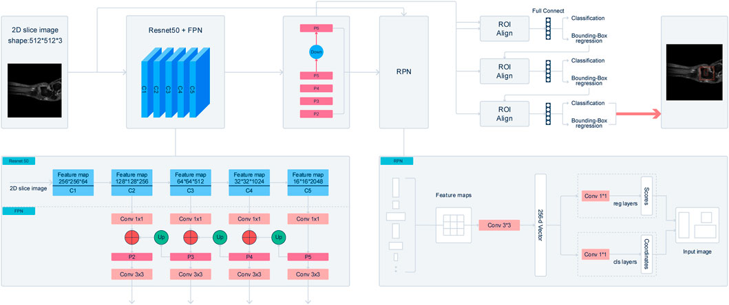
FIGURE 2. Illustraion of Cascade R-CNN architecture. The backbone network extract feature map from 2D slice images. A Residual Neural Network (ResNet50) with feature pyramid network (FPN) is utilized as the backbone of the Cascade-R-CNN. After processing by FPN, a 3*3 convolution layer is added after merging feature maps to get the feature maps, and it is called P2, P3, P4, P5 respectively. In addition, the feature map that is called P6 is got by sub-sampling P5 by a factor 2. The final feature maps are composed of P2, P3, P4, P5, and P6. A window slide over feature maps of multi-scale to obtain a set of predefined bounding boxes that is also called anchors. Anchors is 8* 8, 16*16, 32*32, 64*64, and 128*128 respectively. The feature maps are mapped to a 256-dimensional vector by a 3*3 convolution layer. At last, the anchors that have Intersection-over-Union (IOU) ratio of the anchors and ground-truth boxes, which is greater than 0.5 are selected as proposals boxes. In the third part, the feature map of any box’s proposal is transformed into fixed size by the RoIAlign algorithm. The feature map is fed into 2 concatenated fully connected layers followed by 2 parallel fully connected layers, one of which is used for classification and the other for bounding-box regression.

2.3 Training Details

The network was implemented using PyTorch and trained on one RTX3090 with 24 GB memory. The anchor size of the model is optimized to the sizes [8*8, 16*16, 32*32, 64*64, 128*128], The optimizer for the network was set as SGD (stochastic gradient descent) and the initial learning rate was 0.0125 with a momentum of 0.9. Furthermore, we sat one weight decay of 0.0001 to help with the training stability. To achieve a better model performance, we employed the warm-up training strategy in the training procedure, using an epoch iteration of 5 with an increasing ratio of 0.01. We decreased the learning rate with CosineAnnealing decay strategy and make the learning rate gradually decay from start to finish to fine-tune the final model. Previous research has shown that soft non-maximum suppression (soft-nms) could achieve superior performance on such tasks due to the softer conditions for filtering out boxes. Thus, we implemented soft non-maximum suppression in the inference stage to improve the sensitivity of the model. The property could further help to achieve a good performance of our model. In training, we use online data augmentation that image scale ranges from 0.9 to 1.2 and rotate range from −90 to 90. The total training took 80 epochs to achieve stable convergence results.

2.4 Model Evaluation

In this study, we employed the mean average precision (mAP) as the parameter to evaluate the performance of the proposed model. AP is the area under the precision-recall curve, defined as follows:

$AP= \underset{0}{\overset{1}{{\displaystyle \int }}}P\left(r\right)dr$

where P(r) is the precision-recall curve, and r is the IoU threshold. Then, mAP corresponds to the mean value of AP for multiple-class detection, defined as follows:

$mAP= \frac{1}{N}{\displaystyle \sum A{P}_i}$

AR is two times the area under the recall-IoU curve and it reflects the sensitivity of the model to the target, however in the paper AR is only computed in the case that IoU = 0.5, defined as follows:

$\text{AR}=\text{Recall}\left(\text{IoU}\right),\text{IoU}=0.5$

Then, mAR corresponds to the mean value of AR for multiple-class detection, defined as follows:

$\mathbf{mAR}=\frac{1}{\mathbf{N}}{\displaystyle \sum \mathbf{A}{\mathbf{R}}_{\mathbf{i}}}$

3 Results

Our proposed method for automatic OLT screening based on Cascade R-CNN showed a good performance in predicting the possibility of the disease and detecting the risk areas. Here we detected the osteochondral lesions (Risk Region), the whole talus (Talus) and the gaps (Gaps) at the same time. The AP of predicting Talus, Gaps and Risk Region reached 0.950, 0.975 and 0.550 respectively (Table 2), and the mAP, mAR was 0.825, 0.930 respectively.

TABLE 2

TABLE 2. Quantitative prediction result analysis.

The quantitative results of our model were shown in Table 2. All these parameters indicate that our model achieved an accurate detection performance, suggesting that it could be used for real clinical applications.

The changes of mAP in training model was shown in Figure 3. There are 414 graphs in the training set. Learning the 414 graphs once means an epoch. One mAP value is obtained when each epoch is verified using the verification set once. We tested epoch for 80 times. When the epoch reached the 80th time, the mAP value was approaching 1.0. Figure 3 showed that the rising trend is relatively stable without much fluctuation indicating that the model has been approaching the most optimal solution, and there has been no overfitting phenomenon. In fact, the effect of learning is not becoming better alongwith more rounds of verification because overfitting may occur. In this experiment, because the number of samples is not large, we set the batchsize to 1 to maintain the largest difference of data to resist overfitting.

FIGURE 3

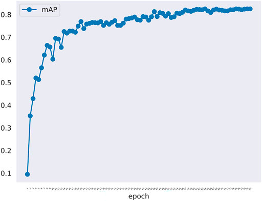
FIGURE 3. The mAP curve in training model along with epoch. The mAP curve rises steadily alongwith the rounds of epoch.

The loss of the training model was shown in Figure 4. The loss denote the sum of all loss of the model. The s0, s1, s2 denote stage1, stage2 and stage3 of the model detector head, in addition loss_cls and loss_bbox denote classification loss and bounding box begression loss. This figure shows the change of loss function in the training model. The blue curve is the sum of the other six curves. So, the blue curve represents the overall loss trend of the model. It can be seen that the curve shows a downward trend. It suggested that less and less information is lost in the training model meaning that the model training is effective. In sumary, we can know that the model alreadly learned something and converged. In addition, model got the nice performance on the validation set.

FIGURE 4

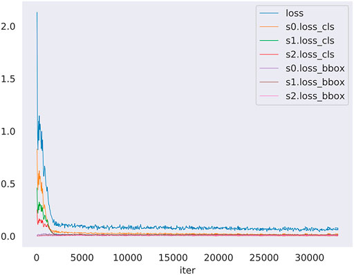
FIGURE 4. The loss curve in training model along with iters. The loss denotes the sum of all loss of the model, moreover s0, s1, s2 denote stage1, stage2 and stage3 of the model detector head, in addition loss_cls and loss_bbox denote classification loss and bounding box begression loss. The blue curve is the summary of the other six curves.

The comparative data between the improved cascade RCNN, which without soft-nms, which without optimized anchor size and faster rcnn was shown in Figure 5 and Tables 3, 4. Small, medium and large denote area of object in range less than 36, 36–96 and greater than 96 repectively. In Figure 5, improved cascade RCNN reach higher value than other models in the last several epochs. In Table 3, the “mAP in all” of “improved cascade RCNN without soft-nms” is highest (0.828). The “mAP in small” of both “improved cascade RCNN” and “improved cascade RCNN without optimized anchor” is heghest (0.225). The “mAP in all” of “improved cascade RCNN without soft-nms” is highest (0.916). However, each mAR categories of “improved cascade RCNN” is highest (0.930, 0.325 and 0.992). In Table 4, talus AP of “improved cascade RCNN” is highest (0.950). Meanwhile, the gap AP and lession AP of “improved cascade RCNN without soft-nms” is highest (0.980 and 0.557). The results showed that the best mAP appeared in training of improved cascade rcnn without softnms, which is higher than the improved cascade rcnn slightly. However, improved cascade rcnn has higher mAR. According to practical application scenarios of the model, the model sensitivity regarding to lesion is of great importance as well. Under the condition that mAP of former is higer than the latter slightly, we can draw a conclusion that the performance of improved cascade rcnn is better than improved cascade rcnn without softnms. In addition, the performance of improved cascade rcnn is better than another model except improved cascade rcnn without softnms.

FIGURE 5

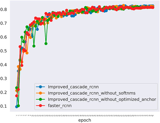
FIGURE 5. The mAP of different models including the improved cascade rcnn, the improved cascade rcnn without soft-nms, the improved cascade rcnn without optimized anchor size. The blue curve indicates the improved cascade rcnn. The orange curve indicates the improved cascade rcnn without soft-nms. The green curve indicates the improved cascade rcnn without optimized anchor size. The red curve indicates the faster rcnn.

TABLE 3

TABLE 3. The comparison of experimental results of optimization method.

TABLE 4

TABLE 4. The comparison of class-wise AP of optimization method.

Furthermore, In the method we use, there are two changes that may have a greater impact on the results. One is the random rotation of data enhancement during training, and the other is the number of epochs. we also compared the mAP and mAR of different changes. In Table 5, all the mAP and mAR categories of “improved cascade RCNN” reached the highest value (0.825, 0.225, 0.894, 0.930, 0.325, 0.992). In Table 6, both talus AP, gap AP and lession AP of ‘improved cascade RCNN’ is highest (0.950, 0.975 and 0.550). Combined with Tables 5, 6, it can be seen from the experiment that the final result of the blue line (i.e. the method we use) is significantly higher than the other two changes (Figure 6). The epoch number 24, is the number of rounds commonly used from imagenet-1k data which was used to get baseline value for training.

TABLE 5

TABLE 5. The comparison of experimental results in different conditions.

TABLE 6

TABLE 6. The comparison of class-wise AP in different conditions.

FIGURE 6

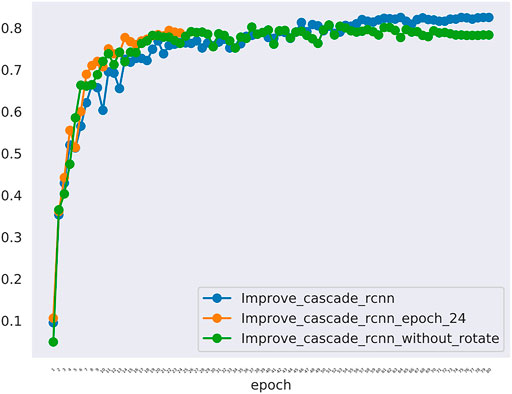
FIGURE 6. The mAP of different models including the improved_cascade_rcnn, the improved_cascade_rcnn_epoch_24, the improved_cascade_rcnn_without_rotate. The blue curve indicates the improved_cascade_rcnn. The orange curve indicates the improved_cascade_rcnn_epoch_24. The green curve indicates the improve_cascade_rcnn without_rotate.

From Figures 7–9, we could intuitively observe that our network provided a comparable detection result (red bounding boxes) with that of senior radiologists (blue bounding boxes). Noticeably, our model achieved stable detection results on all three detection tasks, which shows the effectiveness of our method. More examples are shown in the Supplementary Figures S1–S3.

FIGURE 7

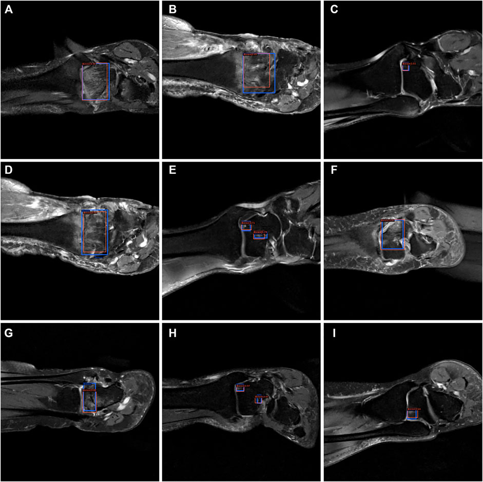
FIGURE 7. The bounding box visualization. Prediction result (red) vs. the ground truth (blue) of the osteochondral lesions. All the images (A–I) were selected from testing group to determine the AI recognition accuracy of ROI. AI detection result was labeled by red rectangular. The ground truth was manually depicted and labeled by blue rectangular.

FIGURE 8

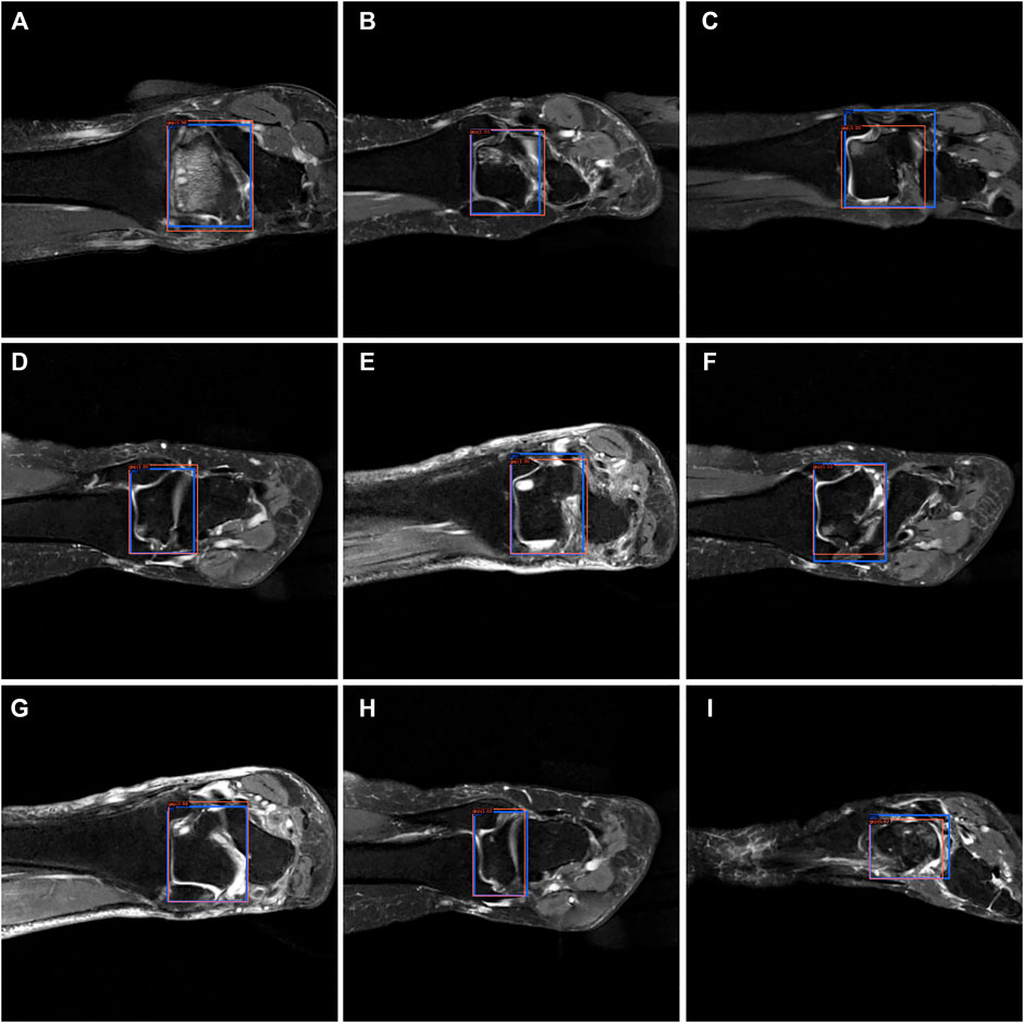
FIGURE 8. The bounding box visualization. Prediction result (red) vs. the ground truth (blue) of the talus gaps. All the images (A–I) were selected from testing group to determine the AI recognition accuracy of talus gap. AI detection result was labeled by red rectangular. The ground truth was manually depicted and labeled by blue rectangular.

FIGURE 9

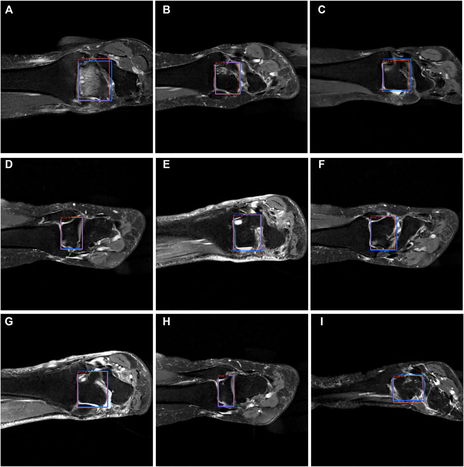
FIGURE 9. The bounding box visualization. Prediction result (red) vs. the ground truth (blue) of the talus itself. All the images (A–I) were selected from testing group to determine the AI recognition accuracy of talus itself. AI detection result was labeled by red rectangular. The ground truth was manually depicted and labeled by blue rectangular.

4 Discussion

For patients who did not benefit from nonoperative management, surgical treatment is indicated, depending on the size, location and chronicity of the lesion. Lesions less than 1 cm in diameter are associated with better outcomes and are amenable to arthroscopic bone marrow stimulation techniques, such as microfractures or subchondral drilling. Autologous chondrocyte implantation (ACI) is indicated for lesions larger than 1 cm in diameter, but it requires 2 stages. Arthroscopy or arthrotomy may be used for the second-stage implantation. For large OLTs with or without bone loss, osteochondral autograft or allograft transplantation may be performed which will cause greater damage and economic burden to patients. Therefore, early screening and early intervention are particularly important.

The initial evaluation of OLTs includes standard radiographs of the ankle and MRI. CT scans are also useful as an adjunct to MRI when evaluating subchondral cysts. Affected by doctors’ experience, the diagnostic accuracy of the same MRI among doctors at various levels is different, which will lead to escaping diagnosis and misdiagnosis. If we can interpret MRI through artificial intelligence, it will greatly improve the diagnostic efficiency and accuracy of patients and reduce the error caused by human factors. The application of artificial intelligence in the field of medical imaging is gradually increasing. In foreign countries, it is mainly divided into two parts: one is image recognition, which is applied to perception whose main purpose is to analyze image data, ROI (region of interest) of image acquisition. The second part is deep learning. Applying deep learning to the studying and analysis is the core segment of AI. Continuous training and deep learning of neural networks through a large number of image data and diagnostic data could achieve a diagnostic model which could enable the AI to master the ability of “diagnosis.” AI will greatly reduce the workload of doctors if better accuracy and specificity can be achieved.

Currently, there are two typical methods to implement the detection project, including the one-stage and two-stage detection methods [23]. Compared with the one-stage method, the two-stage method could achieve a higher detection performance, but at the expense of speed [24]. In order to achieve a higher detection performance, we utilized the two-stage detection methods in this work. Many methods have been proposed in two-stage detection fields, including Mask-R-CNN [25], Fast-R-CNN [26] and Faster-R-CNN [27]. For all the two-stage detection methods, one intersection-over-union (IoU) threshold is required to classify the predicted positive bounding box with the negative bounding box. However, it has been shown that a lower IoU threshold could provide more bounding boxes with a lower precision, which induces a lower recall rate, while a higher IoU threshold could provide fewer bounding boxes with a higher precision, which induces the under detection [28]. To clarify the concept of these statistical terms, the definitions of accuracy, precision and recall rate should be well explained. The predicted condition is usually marked with Positive or Negative. The actual condition is usually labeled with True or False. Subsequently, we have four parts in the contingency table: True positive (TP), False Positive (FP), True Negative (TN) and False Negative (FN). By the use of multiple IoU thresholds, the recently proposed two-stage detection method of the Cascade R-CNN model significantly improved the detection performance compared with the above-mentioned two-stage detection methods. Besides, through multiple regression using cascaded detection heads, the Cascade R-CNN model could further improve the detection precision. The backbone network was built using a ResNet-50 network with pre-trained network weights from the ImageNet dataset, which allowed to fasten the training of the network and improve the final performance.

Our study implemented a deep learning-based method for the automatic detection of osteochondral lesions of the talus for the first time. Our model has achieved an accurate detection with an average, mAP of 0.550, 0.975, and 0.950 on the Risk Region, Gaps and Talus detection tasks, respectively. Compared with other detection tasks, the mIOU reached a similar value to that in a previous study on the detection of coronavirus pneumonia [29] (mIOU, 73.40% ± 2.24%). Furthermore, our model could also provide accurate detection results on multiple risk region parts in one single case without missing any of them. All these results prove that this method could be used by clinical radiologists to overcome the shortness of subjectivity and variability and save the physician’s valuable time.

5 Conclusion

Our research developed a diagnostic model for image interpretation based on artificial intelligence. The detection accuracy of this mode reaches mAP = 0.825. It provides a theoretical basis for the early diagnosis and screening of OLTs based on artificial intelligence detection in the future.

6 Limitation

Although many valuable results have been achieved in this work, there are still some limitations that need to be improved in the future. Firstly, only the articular cartilage on the talar dome was evaluated in our feasibility study, since evaluating the curved articular surface of the talus on the 3.5-mm-thick coronal fat-suppressed proton density-weighted FSE sequence would be challenging. Furthermore, most patients only accept medical consultation and MRI examination at outpatient instead of inpatient. They have no chance to get arthroscopy to make a definite diagnosis. As a result, the presence or absence of cartilage lesions in each image patch was interpreted by a musculoskeletal radiologist. Although arthroscopy has a higher sensitivity for detecting cartilage lesions, arthroscopy was unable to be used as a reference standard in this retrospective study. Meanwhile, only the highest grade of cartilage lesion on each articular surface was recorded in surgery report. However, the exact location of the cartilage lesion was not well described. Even though we extracted 517 slices from 92 patients to implement a deep learning model in this study, which was sufficient enough to conduct a detection task, we could have tried some data augmentation methods to make our model more robust and avoid overfitting greatly. Additionally, having an accurate segmentation map is more desired in many clinical applications to provide a precise treatment plan. However, due to the low resolution of the lesion parts, it was hard for the radiologists to acquire accurate boundaries of the risk region. In future studies, it could be beneficial to include the unsupervised machine learning methods for segmentation tasks in the OLT image analysis. Finally, although we performed the lesions, gaps and talus detection tasks at the same time, some information that was hidden within this structure was still not fully explored and the interpretability of our model was still unknown. In this research, we also conduct a detection task, but in clinical practice surgeons may be focus on the characteristics of lesion (XXX for instance) We believe we could further improve the performance of our model by combining the clinical information with the current detection methods and use a multi-task learning method to perform detection, segmentation, and lesion classification task simultaneously.

Data Availability Statement

The raw data supporting the conclusion of this article will be made available by the authors, without undue reservation.

Author Contributions

QX and JL contributed to the original idea and conceptual design; GW, LZ, and JW conceived the experiments and analyzed data; GW and YC contributed to the drafting of the work; BL, YS, TL and SS provided critical review of the article.

Conflict of Interest

Author TL was employed by Yihui Ebond (Shandong) Medical Technology Co., Ltd. Author SS was employed by Yihui Ebond (Shandong) Medical Technology Co., Ltd.

The remaining authors declare that the research was conducted in the absence of any commercial or financial relationships that could be construed as a potential conflict of interest.

Publisher’s Note

All claims expressed in this article are solely those of the authors and do not necessarily represent those of their affiliated organizations, or those of the publisher, the editors and the reviewers. Any product that may be evaluated in this article, or claim that may be made by its manufacturer, is not guaranteed or endorsed by the publisher.

Acknowledgments

The authors would like to thank EditSprings (www.editsprings.cn), for editing the English text of a draft of this manuscript.

Supplementary Material

The Supplementary Material for this article can be found online at: https://www.frontiersin.org/articles/10.3389/fphy.2022.815560/full#supplementary-material

References

1. Murawski C.D., Kennedy J.G. Operative Treatment of Osteochondral Lesions of the Talus. J Bone Jt Surg Am (2013) 95:1045–54. doi:10.2106/jbjs.L.00773

CrossRef Full Text | Google Scholar

2. Zengerink M, Struijs P.A.A, Tol J.L, van Dijk C.N. Treatment of Osteochondral Lesions of the Talus: A Systematic Review. Knee Surg Sports Traumatol Arthrosc (2010) 18:238–46. doi:10.1007/s00167-009-0942-6

PubMed Abstract | CrossRef Full Text | Google Scholar

3. Kraeutler M.J., Chahla J, Dean C.S., Mitchell J.J., Santini-Araujo MG, Pinney SJ, et al. Current Concepts Review Update. Foot Ankle Int (2017) 38:331–42. doi:10.1177/1071100716677746

PubMed Abstract | CrossRef Full Text | Google Scholar

4. O'Loughlin P.F., Heyworth B.E., Kennedy J.G. Current Concepts in the Diagnosis and Treatment of Osteochondral Lesions of the Ankle. Am J Sports Med (2010) 38:392–404. doi:10.1177/0363546509336336

CrossRef Full Text | Google Scholar

5. Verhagen R.A.W., Maas M, Dijkgraaf M.G.W, Tol J.L., Krips R, van Dijk C.N. Prospective Study on Diagnostic Strategies in Osteochondral Lesions of the Talus. The J Bone Jt Surg Br volume (2005) 87-B:41–6. doi:10.1302/0301-620x.87b1.14702

CrossRef Full Text | Google Scholar

6. LeCun Y, Bengio Y, Hinton G. Deep Learning. Nature (2015) 521:436–44. doi:10.1038/nature14539

PubMed Abstract | CrossRef Full Text | Google Scholar

7. Litjens G, Kooi T, Bejnordi B.E., Setio A.A.A, Ciompi F, Ghafoorian M, et al. A Survey on Deep Learning in Medical Image Analysis. Med Image Anal (2017) 42:60–88. doi:10.1016/j.media.2017.07.005

PubMed Abstract | CrossRef Full Text | Google Scholar

8. Ning Z, Tu C, Di X, Feng Q, Zhang Y. Deep Cross-View Co-Regularized Representation Learning for Glioma Subtype Identification. Med Image Anal (2021) 73:102160. doi:10.1016/j.media.2021.102160

PubMed Abstract | CrossRef Full Text | Google Scholar

9. Peng J, Kim D.D., Patel J.B., Zeng X, Huang J, Chang K, et al. Deep Learning-Based Automatic Tumor Burden Assessment of Pediatric High-Grade Gliomas, Medulloblastomas, and Other Leptomeningeal Seeding Tumors. Neuro Oncol (2021) 24:289–99. doi:10.1093/neuonc/noab151

CrossRef Full Text | Google Scholar

10. Gutman D.C., Young R.J. IDH Glioma Radiogenomics in the Era of Deep Learning. Neuro Oncol (2021) 23:182–3. doi:10.1093/neuonc/noaa294

PubMed Abstract | CrossRef Full Text | Google Scholar

11. Zhang B, Jin Z, Zhang S. A Deep-Learning Model to Assist Thyroid Nodule Diagnosis and Management. The Lancet Digital Health (2021) 3:e410. doi:10.1016/s2589-7500(21)00108-4

PubMed Abstract | CrossRef Full Text | Google Scholar

12. Wu G-G, Lv W-Z, Yin R, Xu J-W, Yan Y-J, Chen R-X, et al. Deep Learning Based on ACR TI-RADS Can Improve the Differential Diagnosis of Thyroid Nodules. Front Oncol (2021) 11:575166. doi:10.3389/fonc.2021.575166

PubMed Abstract | CrossRef Full Text | Google Scholar

13. Wan P, Chen F, Liu C, Kong W, Zhang D. Hierarchical Temporal Attention Network for Thyroid Nodule Recognition Using Dynamic CEUS Imaging. IEEE Trans Med Imaging (2021) 40:1646–60. doi:10.1109/tmi.2021.3063421

PubMed Abstract | CrossRef Full Text | Google Scholar

14. Yoo H, Lee S.H., Arru C.D., Doda Khera R, Singh R, Siebert S, et al. AI-Based Improvement in Lung Cancer Detection on Chest Radiographs: Results of a Multi-Reader Study in NLST Dataset. Eur Radiol (2021) 31:9664–74. doi:10.1007/s00330-021-08074-7

PubMed Abstract | CrossRef Full Text | Google Scholar

15. Wang C, Shao J, Lv J, Cao Y, Zhu C, Li J, et al. Deep Learning for Predicting Subtype Classification and Survival of Lung Adenocarcinoma on Computed Tomography. Translational Oncol (2021) 14:101141. doi:10.1016/j.tranon.2021.101141

CrossRef Full Text | Google Scholar

16. Venkadesh K.V., Setio AAA, Schreuder A, Scholten ET, Chung K, W. Wille MM, et al. Deep Learning for Malignancy Risk Estimation of Pulmonary Nodules Detected at Low-Dose Screening CT. Radiology (2021) 300:438–47. doi:10.1148/radiol.2021204433

PubMed Abstract | CrossRef Full Text | Google Scholar

17. Liu F, Zhou Z, Samsonov A, Blankenbaker D, Larison W, Kanarek A, et al. Deep Learning Approach for Evaluating Knee MR Images: Achieving High Diagnostic Performance for Cartilage Lesion Detection. Radiology (2018) 289:160–9. doi:10.1148/radiol.2018172986

PubMed Abstract | CrossRef Full Text | Google Scholar

18. Kijowski R, Liu F, Caliva F, Pedoia V. Deep Learning for Lesion Detection, Progression, and Prediction of Musculoskeletal Disease. J Magn Reson Imaging (2020) 52:1607–19. doi:10.1002/jmri.27001

PubMed Abstract | CrossRef Full Text | Google Scholar

19. Liu F, Zhou Z, Jang H, Samsonov A, Zhao G, Kijowski R. Deep Convolutional Neural Network and 3D Deformable Approach for Tissue Segmentation in Musculoskeletal Magnetic Resonance Imaging. Magn Reson Med (2018) 79:2379–91. doi:10.1002/mrm.26841

PubMed Abstract | CrossRef Full Text | Google Scholar

20. Cai Y, Landis M, Laidley D.T., Kornecki A, Lum A, Li S. Multi-Modal Vertebrae Recognition Using Transformed Deep Convolution Network. Comput Med Imaging Graphics (2016) 51:11–9. doi:10.1016/j.compmedimag.2016.02.002

CrossRef Full Text | Google Scholar

21. Xue Y, Zhang R, Deng Y, Chen K, Jiang T. A Preliminary Examination of the Diagnostic Value of Deep Learning in Hip Osteoarthritis. PLoS One (2017) 12:e0178992. doi:10.1371/journal.pone.0178992

PubMed Abstract | CrossRef Full Text | Google Scholar

22. Prasoon A, Petersen K, Igel C, Lauze F, Dam E, Nielsen M. Deep Feature Learning for Knee Cartilage Segmentation Using a Triplanar Convolutional Neural Network. Med Image Comput Comput Assist Interv (2013) 16:246–53. doi:10.1007/978-3-642-40763-5_31

PubMed Abstract | CrossRef Full Text | Google Scholar

23. Zhao Z-Q, Zheng P, Xu S-T, Wu X. Object Detection with Deep Learning: A Review. IEEE Trans Neural Netw Learn Syst. (2019) 30:3212–32. doi:10.1109/tnnls.2018.2876865

PubMed Abstract | CrossRef Full Text | Google Scholar

24. Livieratos FA, Johnston LE A Comparison of One-Stage and Two-Stage Nonextraction Alternatives in Matched Class II Samples. Am J Orthod Dentofacial Orthopedics (1995) 108:118–31. doi:10.1016/s0889-5406(95)70074-9

CrossRef Full Text | Google Scholar

25. He K, Gkioxari G, Dollár P, Girshick R. Mask R-CNN. In: 2017 IEEE International Conference on Computer Vision (ICCV); 22-29 Oct. 2017; Venice, Italy. IEEE (2017).

CrossRef Full Text | Google Scholar

26. Girshick R. Fast R-CNN. arXiv e-prints 2015 (2015).

CrossRef Full Text | Google Scholar

27. Ren S, He K, Girshick R, Sun J. Faster R-CNN: Towards Real-Time Object Detection with Region Proposal Networks. arXiv:1506.01497 (2017).

CrossRef Full Text | Google Scholar

28. Jiang B, Luo R, Mao J, Xiao T, Jiang Y. Acquisition of Localization Confidence for Accurate Object Detection. arXiv:1807.11590 (2018).

CrossRef Full Text | Google Scholar

29. Zhang Z, Ni X, Huo G, Li Q, Qi F. Novel Coronavirus Pneumonia Detection and Segmentation Based on the Deep-Learning Method. Ann Transl Med (2021) 9:934. doi:10.21037/atm-21-1156

PubMed Abstract | CrossRef Full Text | Google Scholar