
94% of researchers rate our articles as excellent or good
Learn more about the work of our research integrity team to safeguard the quality of each article we publish.
Find out more
ORIGINAL RESEARCH article
Front. Phys., 12 April 2022
Sec. Medical Physics and Imaging
Volume 10 - 2022 | https://doi.org/10.3389/fphy.2022.813475
This article is part of the Research TopicCapturing biological complexity and heterogeneity using multidimensional MRIView all 9 articles
 Yiqiao Song1,2*
 Ina Ly3
 Qiuyun Fan1,4
 Aapo Nummenmaa1
 Maria Martinez-Lage5
 William T. Curry6
 Jorg Dietrich3Deborah A. Forst3
 Bruce R. Rosen1
 Susie Y. Huang1Elizabeth R. Gerstner3
Diffusion MRI is widely used for the clinical examination of a variety of diseases of the nervous system. However, clinical MRI scanners are mostly capable of magnetic field gradients in the range of 20–80 mT/m and are thus limited in the detection of small tissue structures such as determining axon diameters. The availability of high gradient systems such as the Connectome MRI scanner with gradient strengths up to 300 mT/m enables quantification of the reduction of the apparent diffusion coefficient and thus resolution of a wider range of diffusion coefficients. In addition, biological tissues are heterogenous on many scales and the complexity of tissue microstructure may not be accurately captured by models based on pre-existing assumptions. Thus, it is important to analyze the diffusion distribution without prior assumptions of the underlying diffusion components and their symmetries. In this paper, we outline a framework for analyzing diffusion MRI data with b-values up to 17,800 s/mm2 to obtain a Full Diffusion Tensor Distribution (FDTD) with a wide variety of diffusion tensor structures and without prior assumption of the form of the distribution, and test it on a healthy subject. We then apply this method and use a machine learning method based on K-means classification to identify features in FDTD to visualize and characterize tissue heterogeneity in two subjects with diffuse gliomas.
Diffusion MRI (dMRI) is capable of characterizing tissue microstructure and differentiating between different types of tissues in diseases of the central nervous system [1–5]. This is because water diffusion is hindered or restricted by the presence of cells, blood vessels and other structures inside tissues. Thus, these diffusion properties can be used to characterize tissue structure. For example, water molecules inside axons can diffuse relatively freely along the axon axis, however, the diffusion perpendicular to the axon axis is more restricted. As a result, angular measurement of the diffusion coefficient allows MRI (e.g., diffusion tensor imaging (DTI) [6, 7]) to identify axon directions and white matter tracts [8] and other tissues [9, 10]. Pathologic tissues (such as brain tumors) exhibit different microstructural properties compared to normal tissue, therefore resulting in altered water diffusion (e.g. [11–13]). In addition, molecular diffusion properties reflect the molecular composition as well as the physical and fluidic environment. For example, when a water molecule is present in viscous fluid, its diffusion coefficient will be reduced. In the existing MRI literature, anisotropic diffusion properties are often described by a diffusion tensor, D, defined as a 3-by-3 matrix,
Mathematically, D is a symmetric tensor, so that Dxy = Dyx, Dxz = Dzx, and Dyz = Dzy. The diffusion tensor can be diagonalized in its eigenvector space where D is a diagonal matrix with eigenvalues λ1, λ2, λ3. For tissues, we expect these eigenvalues to vary broadly both in values and symmetry.
In dMRI, such as DTI [6, 7], the MRI signal can be described as:
where M0 is the signal when b = 0, D is the diffusion tensor and b is the diffusion weighting b-tensor, and the expression b: D indicates a tensor product [2, 6]. In tissues, many different microstructural components are often present within a single voxel of the image. These different components exhibit different values of the diffusion coefficient values, so that the total signal is the sum of all components [14–18],
Here Dj, and fj are the diffusion tensor of the j-th component and its weight, and N is the total number of components. For example, it is common in neuroimaging to consider three components [19]: 1) the signal associated with axons with an anisotropic diffusion behavior, 2) the signal associated with the tissue in which the diffusion is restricted isotropically, and 3) the signal from an unrestricted water pool [20, 21]. These three water compartments (or pools) grossly reflect the structure of brain tissue but represent an oversimplified model. This is because, even within the same water population, the details of the tissue microstructure may vary, including axon diameters, axonal orientation, and the degree of restricted diffusion. As a result, it is necessary to expand this model to beyond only a few components to accurately describe the underlying tissue microstructure. The goal of this work is to develop a method that captures all possible diffusion tensors in biological tissues with no a priori exclusion of certain diffusion tensors or limit on their amplitudes.
However, Eq. 3 belongs to a class of integral equations that are mathematically ill-conditioned and difficult to solve for noisy experimental data [22] in the sense that small changes in the data noise can cause significant changes in the resulting fi. This inversion stability can be improved by imposing constraints on the obtained distributions, e.g., by fixing the diffusion tensor eigenvalues and solving for the orientation distribution function (ODF) or only considering a few components with pre-defined or heavily constrained diffusivities [19, 21, 23–25]. For example, the RSI model (Restriction Spectrum Imaging [21]) includes 12 axially symmetric diffusion tensors and analyzes the fiber orientation distributions of different diffusion components to demonstrate its potential in visualizing tumor cellularity and white matter tracks around brain tumors [13]. Other methods have applied constraints to the potential functional forms of the diffusion properties based on the understanding of tissue microstructures, e.g., Refs. [26–29]. Although these constraints facilitate data inversion and are necessary given the limited range of b values available on clinical MRI scanners, they often rely on assumptions that are difficult to fully justify, which may give rise to bias and errors [30, 31]. In this work, we leverage the higher gradients afforded by the Connectome scanner with b-values up to 17,800 s/mm2 [32–35] to better characterize tissue microstructure in normal human brain and diffuse gliomas. We accomplish this by further eliminating the restriction on diffusion tensors and the functional forms of the distribution and thus obtaining a full diffusion tensor distribution (FDTD). We further used a data-driven method, K-means clustering algorithm [36] to visualize the tissue heterogeneity in the diffuse gliomas.
To obtain a comprehensive description of tissue properties using Eq. 3, we expand the definition of diffusion tensor components to include those with and without axial symmetry. It is common to order the eigenvalues in an ascending order, i. e., λ1 ≤ λ2 ≤ λ3. In this coordinate frame, if two eigenvalues are equal, then the tensor is considered to be axially symmetric. For example, because of the cylindrical symmetry of the axons, the diffusion tensor for axon water is considered axially symmetric. Furthermore, since the geometric restriction is along directions transverse to the axon axis, the diffusion tensor for axons is generally believed to be characterized by:
Such symmetry with a strong anisotropy has been observed in many white matter regions where the axon bundles are highly aligned. However, the diffusion anisotropy varies throughout white matter regions. In gray matter regions, the voxel-averaged anisotropy can be quite low due to the broad orientation distribution of axons. In white matter regions, there can be a significant variation of axon diameter [37–39].
In order to accurately characterize brain tissue, we explicitly consider a wide range of λ1, λ2, λ3 without restricting them to certain symmetries or their numerical values, in order to capture all possible diffusion tensors within the range:
where dmin and dmax are the minimum and maximum value of the diffusion coefficient allowed in the analysis. For example, dmax = 3*10−3 mm2/s, which is approximately the diffusion coefficient of water at normal human body temperature. On the other hand, dmin can be set to zero, or 1/100 of dmax.
A few special cases of the diffusion tensor should be mentioned explicitly. For the D with identical three eigenvalues, λ1 = λ2 = λ3, the diffusion tensor is isotropic, i.e., diffusion along any direction will be identical, such as for bulk water, or water in very large pores. For example, diffusion in the ventricles of human brain exhibits such isotropic behavior. For the D with λ1 = λ2 < λ3, it is often called a prolate spheroid. In particular, when the anisotropy is large, the shape is like a needle. For the D with λ1 < λ2 = λ3, it is often called an oblate spheroid which has a disc-like shape. In the analysis of dMRI, the use of a prolate spheroid (needle-like shape) to model the axon is common. However, the oblate spheroid (disc-like shape) or other shapes in particular with three different eigenvalues (λ1 ≠ λ2 ≠ λ3) are not often used in previous DTD (diffusion tensor distribution) models. Jian et al. [23] and Magdoom et al. [29] have proposed to include oblate and other anisotropic tensors, however, constrained the DTD to certain predefined functions. Herberthson et al. [40] also studied the generalized diffusion tensor for orientationally averaged dMRI data.
Within an MRI voxel of tissue, multiple types of tissue may exist concurrently and thus the MRI signal is a sum of all the different types of tissues that are characterized by their diffusion tensors, D:
Here, f(D) is the full diffusion tensor distribution (FDTD) function, which is proportional to the amount of water molecules with a specific diffusion tensor D and ∫dDf(D) = 1. b is the diffusion weighting factor that is determined by the MRI pulse sequence, in particular the field gradient pulses to provide diffusion sensitivity. Specifically, the gradient pulses are applied along different directions (for example based on the Q-Ball method [41]) and b is described by a tensor [2, 6]. The integration is over all the independent tensor elements, and can be performed over the eigenvalues (λ1, λ2, λ3) and orientations (the corresponding Euler angles) of the diffusion tensor.
In order to obtain the full diffusion tensor information which includes the magnitude of the diffusion coefficients and the orientation of the eigenvectors, it is necessary to acquire MRI data for a wide range of diffusion weightings b, and the direction of the gradients. For clinical examinations, the commonly used DWI (diffusion weighted imaging) method is usually performed with a single b value. These DWI data cannot be used to obtain FDTD. Similarly, single-shell DTI or diffusion kurtosis MRI data (DKI) [42] are insufficient to obtain high quality FDTD. Instead, DTI (or diffusion-weighted) acquisition with more than three b-value shells is needed. For our experiments, up to 8 b-value shells were used with b-values from zero up to 17,800 s/mm2. The large b-values are useful to identify the components with low diffusion coefficients. Since the expected diffusion coefficient spans a very large range, b values should also span a correspondingly large range. For our experiments, 32–64 different directions for each gradient value were used. More directions used in the measurement would improve the angular resolution of the FDTD but this would occur at the expense of longer scan times. The key advantage of the Connectome scanner is the ability to achieve better signal-to-noise ratio (SNR) at high b values than conventional MRI scanners so that the entire diffusion-induced signal decay can be observed.
In this Institutional Review Board-approved study, three participants (one healthy subject, two subjects with diffuse gliomas) provided written informed consent. All subjects were scanned on a high-gradient 3 Tesla MRI scanner (MAGNETOM CONNECTOM, Siemens Healthcare, Erlangen, Germany) with a maximum gradient strength of 300 mT/m using a 64-channel head coil [43]. For the healthy subject, the multishell acquisition consisted of two diffusion times (19 and 49 ms) and eight gradient strengths per diffusion time, which were linearly spaced from 30 to 290 mT/m with a maximum b value of 17,800 s/mm2. Diffusion-weighted images were acquired with spatial resolution of 2 × 2 × 2 mm3 voxels, echo time/repetition time = 77/3,600 msec, parallel imaging acceleration factor R = 2, simultaneous multislice imaging with a slice acceleration factor of 2, and anterior-to-posterior phase encoding. Interspersed b = 0 images were acquired every 16 images. The total acquisition time for the dMRI of one diffusion time was about 24 min. Further details of the protocol can be found in Refs. [38, 39]. For glioma patients, 4 and 5 gradient increments were used for the two diffusion times respectively with a similar b value range. Additionally, T1-MPRAGE and T2-SPACE-FLAIR sequences were obtained with a total scan time of about 56 min. Both glioma patients had non-enhancing T2/FLAIR-hyperintense tumors. Thus, the T2/FLAIR-hyperintense region was defined as the tumor region of interest (ROI).
Once the multishell DTI images are obtained, the signal for each voxel can be written as a vector, S = si, where i is the index of the experiments covering all b-values and gradient orientations. Eq. 6 may be re-written in a matrix form:
where S is the data vector, F is FDTD in a vector form (e.g., Fj is the j-th component of FDTD), and K is the kernel function that is defined as
Here the index i corresponds to the i-th experiment with bi, and j is the index of the j-th diffusion tensor. A diffusion tensor is characterized by the three eigenvalues and the three Euler angles (α, β, γ):
In our formulation, Fj corresponds to the signal weight for the Dj component and the length of F and D is the same. In order to achieve a comprehensive representation of the diffusion tensors, the range of Dj should be quite large. For example, we typically discretize the eigenvalues and the Euler angles as follows:λ1, λ2, λ3: each from 3 × 10⁻⁵ to 3 × 10⁻³ mm2/s, in 10 steps in log space; α, β, γ: each from 0 to 180 or 90°, in 10 steps. As a result, the total number of diffusion tensor components can be very large, e.g.
Here we show four simulation examples using the FLI inversion algorithm (Figure 1) and all simulations were performed using the protocol for the healthy subject. First, we consider a two-component system (model 1) with an isotropic diffusion tensor λ1,2,3 = 10−3 mm2/s, and an anisotropic tensor with λ1,2 = 0.05 × 10⁻³ mm2/s, and λ3 = 2 × 10⁻³ mm2/s. Such a diffusion tensor has a fractional anisotropy (FA) of 0.96, as the FA for an intact axon can approach unity [48] similar to that of the highly anisotropic white matter regions (discussed later in Section 3.1). The dMRI signal is simulated with b vector for the healthy volunteer (in Section 2.2) shown in Figure 1A. The inversion results are displayed in 2D projections in Figures 1B–D. The model values of the eigenvalues are illustrated in Figures 1B–D to highlight the consistency of the inversion results with the models. The second model (model 2) considered is 5 axons oriented along different orientations in the X-Z plane, λ1,2 = 0.1 × 10⁻³ mm2/s, and λ3 = 2 × 10⁻³ mm2/s. The inversion result (Figures 1F–H) is able to identify a single components of high anisotropy of the intrinsic diffusion tensor, consistent with the model as illustrated by the agreement with the red circles.
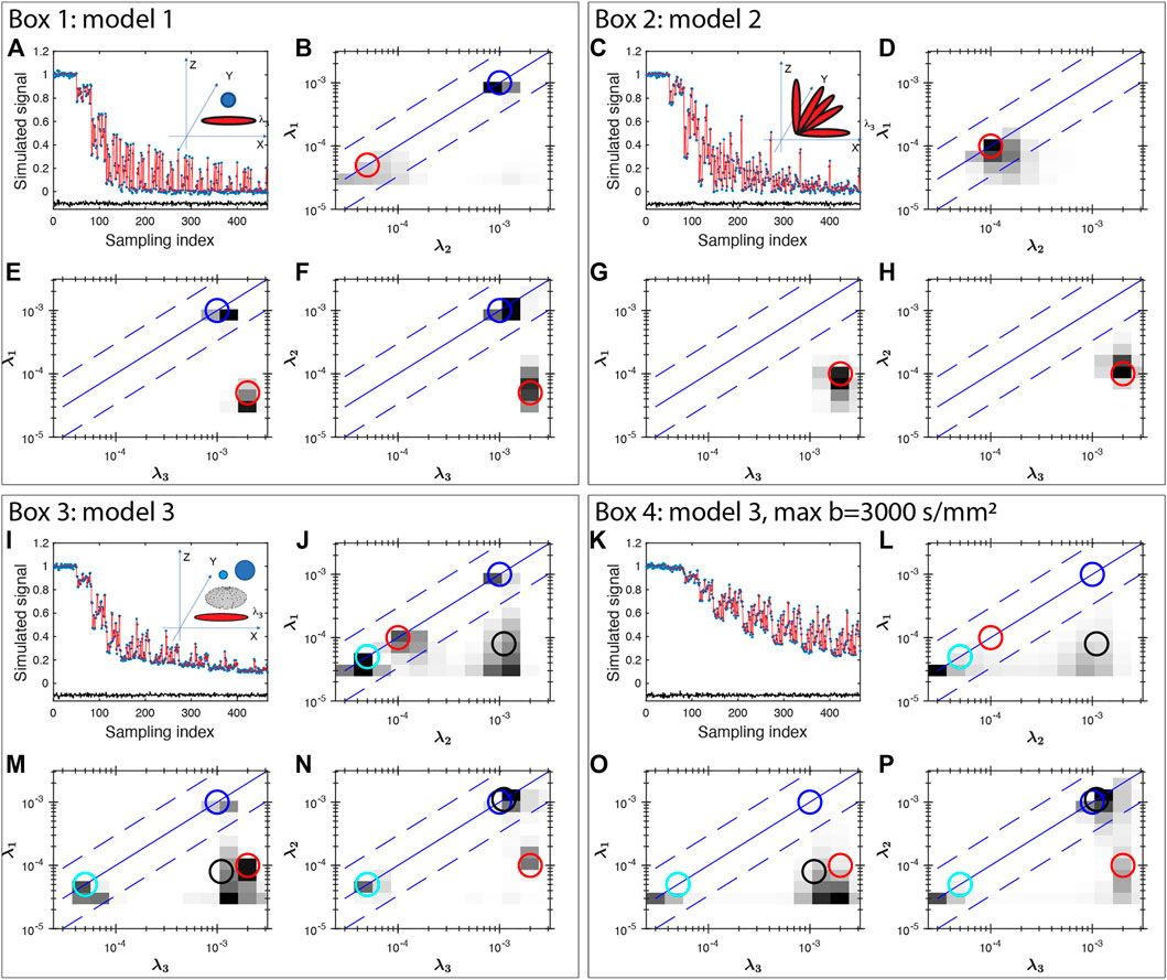
FIGURE 1. Multishell DTI signal simulation and inversion results for three models of diffusion tensors (Box 1–4). Gaussian noise of 0.01 amplitude was added to the simulated signals. The unit for the eigenvalue axes is mm2/s. In Box 1, two components of diffusion tensors are simulated, one isotropic and one anisotropic. In Box 2, five anisotropic tensors with different orientations are considered. Box 3 considers four diffusion tensors: two isotropic tensors (blue and cyan), one prolate (red) and one oblate (black) tensor. Box 4 uses the same model as Box 3 and shows the results with a maximum b value of 3,000 s/mm2 exhibiting significant broadening. In each Box, the top-left panel show the simulated data (blue stars), fitting (red line) and the fit error (black line, shifted vertically by −0.1 for clarity) demonstrating a uniform fit residue for all data points. The insets in the top-left panel also shows the model of diffusion tensors. Other panels show the 2D projections of diffusion tensor eigenvalue distributions. The circles (blue and cyan for isotropic signals, red for axon-like signals, black for oblate tensor) indicate the model values of the projections demonstrating the consistency between the models and the inversion results for all simulations.
We further consider a model 3 that include two isotropic water compartments, with λ1,2,3 = (0.05, 1) × 10−3 mm2/s, one prolate tensor: λ1,2 = 0.05 × 10⁻³ mm2/s, and λ3 = 2 × 10⁻³ mm2/s, and oblate tensor: λ1 = 0.08 × 10⁻³ mm2/s, and λ2,3 = 1 × 10⁻³ mm2/s and the results are shown in Figure 1I–L. Panel J–L show a reasonable consistency between the model (circles) and the inversion result, however, significant broadening is observed near the low diffusion coefficient areas. Similar broadening is also seen in Panel F and J for the model 2 with 5 axons. This broadening is more severe when the maximum b value is smaller, such as bmax = 3,000 s/mm2 shown in Figure 1M–P. Such resolution limitation is related to the ill-conditioned nature of the diffusion kernel function and the available SNR of MRI data [49]. Similarly, there can be considerable uncertainty and broadening in determining diffusion tensor anisotropy (e.g. shown in Refs. [2, 50]). This is particularly true if one is trying to interpret a specific peak position, or amplitude at a specific diffusion coefficient. Thus, we use integrals of FDTD as defined in the following equation in our additional analysis to identify tissues types, i. e:
where the p(D) is the parameter defined as a function of D, and the integral is performed over the diffusion tensor space. For example, signals related to axons can be defined as p = 1 only for the high anisotropic D similar to a needle. The specific definition of p used in this paper is described in the Table 1 above.
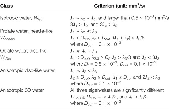
TABLE 1. Definition of the integration space used in Eq. 10 for the different classes of signals.
In addition to help the visualization of the 3-dimensional diffusion tensor distribution, the uncertainty of such integrals ϕ will be much reduced [51, 52] as compared with that of an individual tensor. This behavior is common in ill-conditioned problems due to the exponential functional form. An integral function of the distribution Eq. 10 will show less uncertainty because the amplitudes of similar decay components (such as diffusion coefficient, T1 and T2) are often anti-correlated [53]. An example is the integral over the entire diffusion coefficient space which equals the total signal, a completely well-conditioned parameter.
To further visualize the FDTD analysis, a K-means clustering algorithm [36] was applied to classify tissues. The main application of the K-means method is to optimally group the data points into several clusters so that the data points within a cluster are closer (more similar) to their center (centroid) than to other clusters. The K-means method has been used widely and there are many easily accessible introductory text on this topic (e.g. wikipedia, https://en.wikipedia.org/wiki/K-means_clustering). Here we will describe our implementation using Matlab (Mathworks, Natick MA). First, the three angular dimensions of the full 6-dimensional FDTD matrix F are integrated to yield a three-dimensional matrix F3. This step reduces the data size substantially to speed up the subsequent calculation, and it also focuses the classification on the microscopic tissue properties instead of the orientation of the tissues. In the second step, a volume of F3 data is formatted to use the kmeans function in Matlab:
[kmap,C] = kmeans(F3,nCluster),
where F3 is the input data matrix reformatted to conform to the syntax of kmeans function, nCluster is the number of clusters to perform K-means algorithm, C is the resulting list of centroids, and kmap is the classification result.
As an input parameter, nCluster is chosen empirically. We applied the K-means algorithm for nCluster = 1 to 10 and calculated the WCSS (Within-cluster-sum-of-squares) which describes the average distance of the data points to the centroids. The results are shown in Figure 2 with a gradual decay of WCSS. At nCluster = 5, WCSS decay is reasonably flattened and is about 10% from its asymptote at large nCluster. Furthermore, at larger nCluster’s, the resulting K-means map becomes progressively unstable, a sign of over fitting. For the further analysis in this work, we choose nCluster = 5 to obtain five tissue clusters: c1, c2, c3, c4 and c5 and the kmeans algorithm assigns every voxel to one of the clusters (c1-c5).
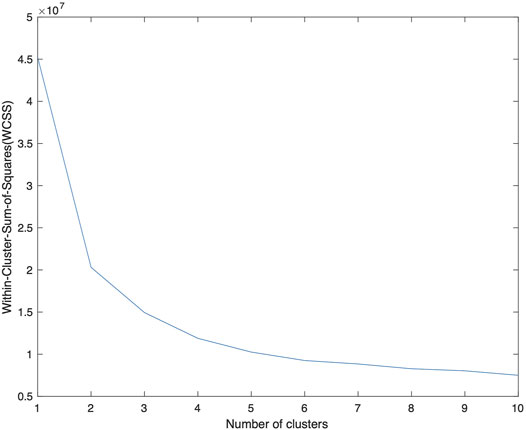
FIGURE 2. A plot of WCSS of the resulting K-means analysis as a function of nCluster, on the F3 data from patient number 1. The decay of WCSS slows down at nCluster = 4 and is flattened at larger nCluster. A choice of nCluster = 5 is made to provide a stable K-means map. The centroids obtained from this data is applied to the data from other patients.
We used the F3 data from Patient 1 to obtain the centroids Cp1 of the 5 clusters. We then applied the same centroids to the F3 data of Patient 2 using the following Matlab syntax:
[kmap, C, sumd] = kmeans(F3,nClass,‘MaxIter’,1,‘Start’,Cp1).
Since the maximum iteration (MaxIter) is only 1, the algorithm classifies the new data (F3) using the input centroid Cp1, but does not further change the centroid.
Figure 3A shows the raw dMRI image for a healthy volunteer and the inversion FDTD results to visualize the different patterns of water distribution. For example, the isotropic water signal (Figure 3B) is concentrated in fluid-filled areas, such as the ventricles and sulci along the brain surface. Strong signals with prolate (needle-like) symmetry (Figure 3C) are found along white matter regions (e. g. corpus callosum). Oblate water (disc-like) signal (Figure 3D) is not commonly used to analyze dMRI, but is seen throughout the brain. It is interesting to note that oblate water is absent in the corpus callosum. Anisotropic disc-like water (Figure 3E) is similar to oblate symmetry except that λ2 and λ3 are significantly different, and is characterized by a uniform spatial distribution throughout the brain except in the ventricles. This spatial distribution is very different from that of the oblate water. Figure 3F exhibits a weak signal of the anisotropic diffusion tensor suggesting that such symmetry may not be important for healthy brain tissues.
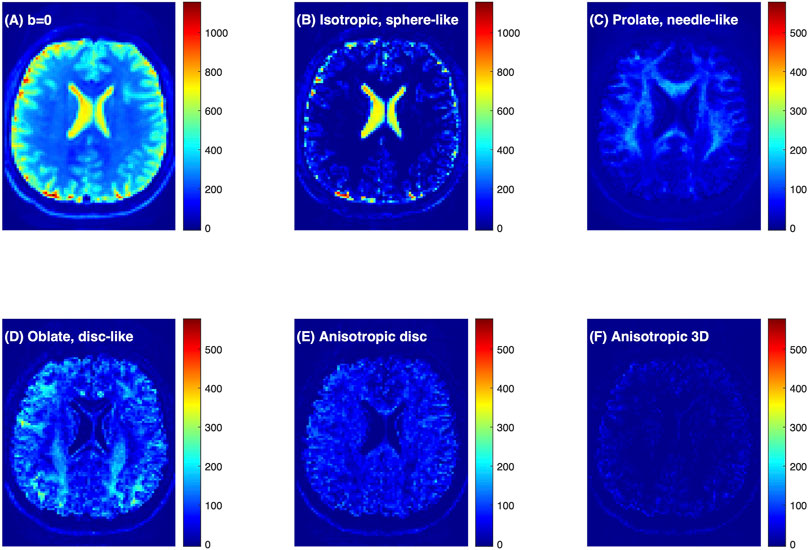
FIGURE 3. Connectome dMRI image of a healthy volunteer and the results of FDTD analysis. (A) dMRI raw image at b = 0 s/mm2. (B–F) Images of the water signals classified based on diffusion tensor properties. Detailed definition of the water fractions can be found in the text. The colorbars indicate signal intensity and highlight the relative scale between the panels.
Figures 4A–D shows a comparison of FDTD with maps of fractional anisotropy (FA) from a conventional DTI analysis. Among the three FDTD panels, Wneedle map shows a close similarity to the FA map. This is understandable since the signal for both FA and Wneedle is mostly derived from axons with strong diffusion anisotropy. This is most clearly demonstrated in area where FA approaches 1, such as at the diamond position in Figure 4B1–4 (FA = 0.93), where the FDTD indicated a strong signal of Wneedle ∼ 0.88 and little signals from other water pools (Wiso ∼ 0 and Wdisc ∼ 0.01). In a low FA area (as indicated by the circle) in Figure 4B1–4, FA = 0.11, we found that Wiso and Wdisc are significantly stronger and Wneedle ∼ 0.06 is low, suggesting that tissue microstructure and composition are very different from areas with high FA (see diamonds).
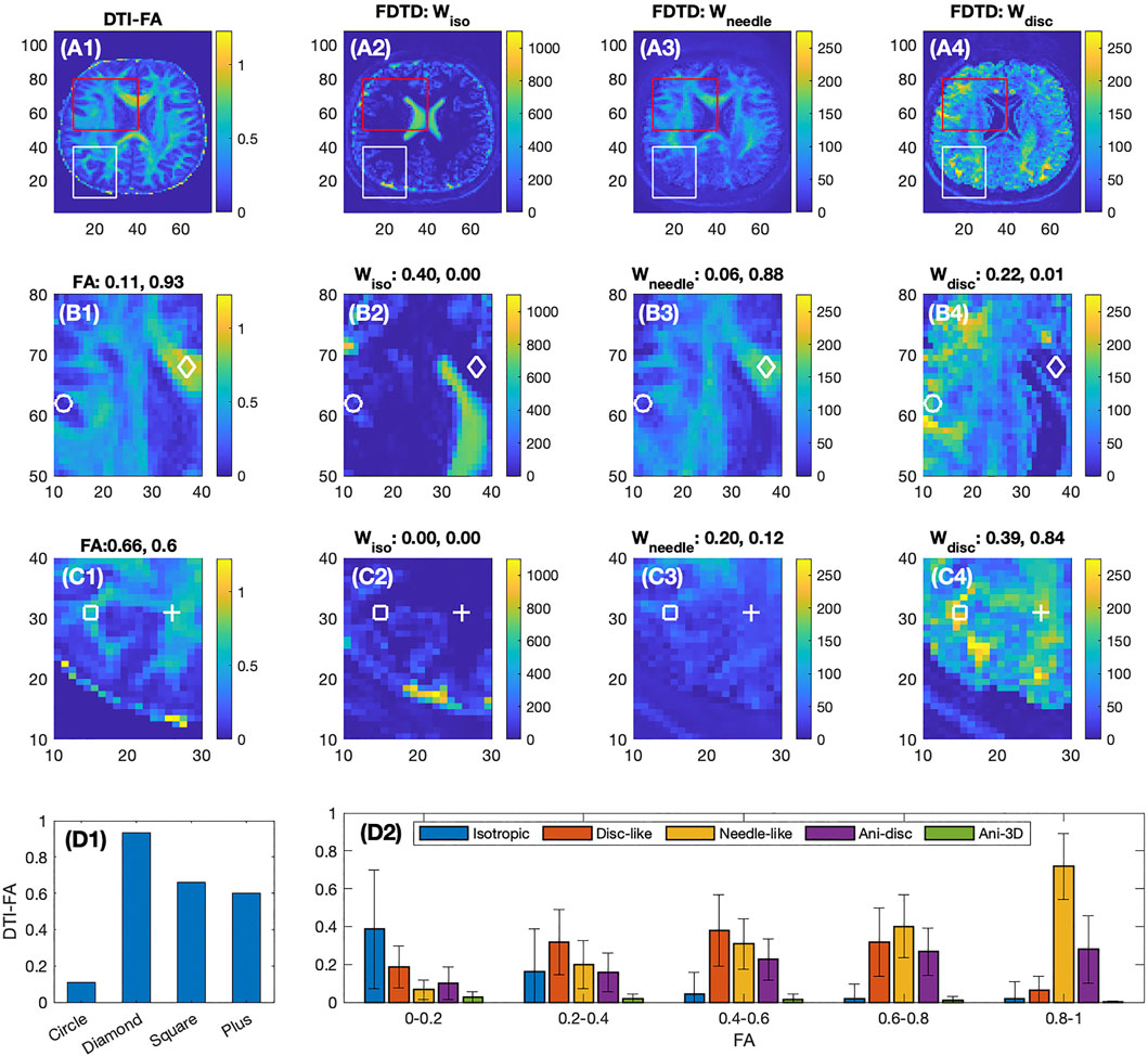
FIGURE 4. Comparison of DTI-FA image with FDTD of the healthy volunteer. First row shows the full frame images, second and third rows show the expanded images indicated in the red and white boxes, respectively. The four columns show the images of FA derived from DTI analysis, and Wiso, Wneedle, Wdisc from FDTD analysis, respectively. For Panels (B2–4) and (C2–4), each plot denotes the fraction of the respective signal normalized by the total signal measured at the four positions indicated by the circles, diamonds, squares and pluses. The colorbars indicate the signal intensity scale and highlight the relative scale between the panels. Panel (D1) shows the FA values at the four positions. Panel (D2) shows the average fractions of the five water pools at different FA ranges.
On the second row (Figure 4B1–4), the ventricles are well identified in panel B2, and the corresponding areas in B3 and B4 show a very low signal in both Wneedle and Wdisc. On the other hand, the near-zero FA region (B1) is much larger than the ventricle defined by B2. As a result, the FDTD result is able to resolve a greater degree of tissue detail in this area (FA
The third row (Figure 4C1–4) focuses on areas with intermediate FA, e. g. FA ∼0.6 at the square and plus positions where both show zero Wiso, but intermediate Wneedle and stronger Wdisc. Furthermore, the Figure 4C1 shows a clear pattern of FA while the maps of Wneedle and Wdisc are much more spread out. The averages of these fractions are shown in Figure 4D2 plotted as a function of FA ranges. For example, the isotropic water fraction is found to decrease to zero as FA increases, and the Wneedle increases gradually and dominates as FA approaches unity. In the intermediate FA, several types of tissues contribute with similar weights. The error bars indicate the range of the fractions in each FA range.
Diffuse gliomas originate from glial cells within the central nervous system and include histologically benign and malignant tumors [54]. They are spatially heterogeneous (characterized by areas of infiltrating and solid tumor cells, necrosis, hypoxia, and vasogenic edema) and diffusely infiltrate surrounding brain tissue. While low-grade (World Health Organization (WHO) grade 2) gliomas are typically slow growing, high-grade (WHO grade 3 and 4) gliomas (including glioblastomas) are aggressive tumors and associated with a dismal prognosis [55, 56]. Accurate delineation of tumor extent to assist with surgical and radiation therapy planning as well as longitudinal monitoring of the tumor resection cavity and residual tumor are important to improve treatment outcomes.
We analyzed dMRI data of two patients with diffuse gliomas: Patient 1 had a WHO grade 3 anaplastic astrocytoma and Patient 2 had a WHO grade 2 oligodendroglioma. Both tumors were isocitrate dehydrogenase (IDH)-mutant, denoting a somatic molecular alteration that confers improved prognosis compared to diffuse gliomas that are IDH-wild-type [57–60]. Both tumors lacked contrast enhancement after gadolinium administration and were T2/FLAIR-hyperintense.
The FDTD results from Patient 1 are shown in Figures 5A–F. Panel A and B show the raw DTI images at b = 0 and 2,600 s/mm2 (averaged over all gradient orientations). The red outlines in each panel delineate the T2/FLAIR-hyperintense region, which is defined as the tumor region of interest (ROI). The tumor ROI exhibits increased signal at b = 0 s/mm2, which decays greatly at b = 2,600 s/mm2 in the central region of the tumor, reflecting the presence of highly diffusive components. This strong signal decay in the central portion of the tumor (compared to contralateral normal brain) suggests the presence of fewer tissues with restricted diffusion (such as axons) in this region.
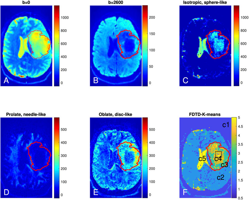
FIGURE 5. Brain dMRI images and FDTD analysis of Patient 1 with grade 3 glioma. (A,B) Brain diffusion MRI images at b = 0 and 2,600 s/mm2 (averaged over all gradient orientations); (C–E) Images of three pools of water signals from the FDTD analysis. (F) Image of the tissue classification from K-means analysis (c1-c5). The red lines indicate the perimeter of the cancer region. The black box in tumor center (F) indicates the position from where the histopathologic sample was obtained.
Figure 5C shows the presence of isotropic water, which is highly diffusive (thus less restricted) and related to free water. This isotropic water signal is strongest in the cerebrospinal fluid-filled ventricles (Figure 3). In addition, there is a significant amount of isotropic water in the center of the tumor (Panel C). Figure 5D shows the prolate (needle-like) water signal, which is due to a highly anisotropic diffusion tensor and related to water in axons or other highly directional structures. Figure 5D shows a reduction of prolate water signal within the center of the tumor ROI compared to contralateral normal brain, suggesting that axonal structures are absent in this area. A similar pattern of fewer axonal structures in the center of gliomas has been reported using a DTI fibre tracking technique [61]. Lastly, Figure 5E shows accumulation of the oblate water signal along the lateral margins of the tumor ROI. Given the different symmetry of the oblate diffusion tensor, this suggests that the tissue microstructure along the tumor periphery differs from that within the center of the tumor.
FDTD analysis provides a comprehensive voxel-wise characterization of tissue for each voxel. However, the resulting FDTD dataset is very large (e. g. half a million data points per voxel) and difficult to visualize. The integration of a few types of tensor symmetry, as described for Figure 5 is a more practical approach. On the other hand, such an approach is influenced by the simplified assumptions of the underlying tissue microstructure, e. g. to focus on signals with an axial symmetric diffusion tensor to characterize axons. This is the bias that we would like to avoid. To continue our approach of unconstrained diffusion tensors, we choose to use a numerical classification method, K-means, to identify features in FDTD without direct assumption.
The K-means result kmap with nCluster = 5 is shown in Figure 5F with five tissue clusters: c1, c2, c3, c4 and c5, as illustrated in different colors. For Patient 1, c5 is present in the ventricles where the signal is derived from cerebrospinal fluid. c4 and c3 are found within the tumor ROI where c4 highlights the central tumor ROI and c3 is predominantly found along the tumor periphery. It is interesting to note that c3 and c4 localized well to the tumor ROI using the K-means algorithm without the algorithm knowing about the T2/FLAIR data or the tumor ROI. There are also voxels of c5 within the tumor center (Panel F and other slices). Overall, c4 and c5 reside in the central region of the tumor ROI and c3 covers the peripheral tumor ROI. c2 corresponds to normal brain and c1 localizes to regions outside the brain. The results from the K-means clustering analysis are consistent with our heuristic discussion above that identifies distinct types of tissue in the center and periphery of the tumor. The key difference is that our heuristic relies partly on the conventional understanding of brain tissue structure while the K-means method derives the result from the F3 data only, in keeping with our approach.
The results for Patient 2 are shown in Figure 6 in a format similar to Figure 5. The raw diffusion images show the significant signal reduction in the tumor area at b = 2,600 s/mm2, similar to Patient 1. The FDTD analysis illustrates the presence of free water only in a small part of the tumor. Similar to Patient 1, the needle-like signal is also reduced significantly in the center of the tumor; while the disc-like signal is rather strong in the tumor. The K-means cluster analysis further classified the tissue in the tumor ROI to be mostly c3 (green) and, to a lesser extent, c4. A small portion of the tumor ROI is found to be c2. Note that there are some voxels to be classified to be c4 around the white circle. The white circle indicates the area where biopsy was obtained to establish a diagnosis of a grade 2 oligodendroglioma.
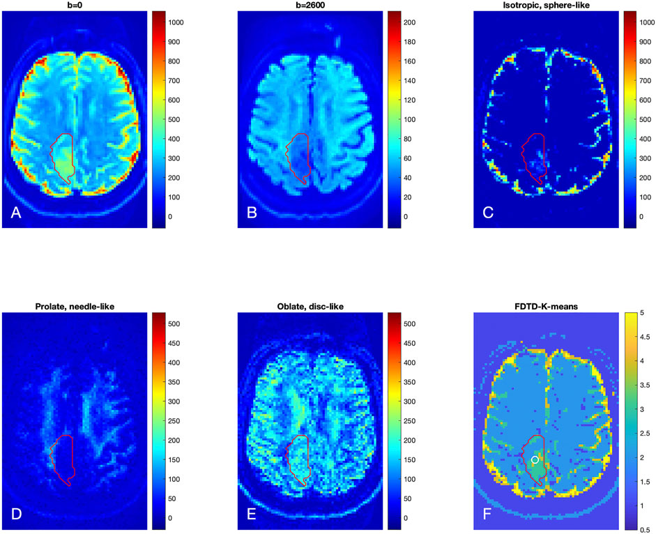
FIGURE 6. Brain dMRI images and FDTD analysis of Patient 2 with grade 2 glioma. (A,B) Brain diffusion MRI images at b = 0 and 2,600 s/mm2 (averaged over all gradient orientations); (C–E) Images of three pools of water signals from the FDTD analysis. (F) Image of the tissue classification from K-means analysis, showing primarily c3 within the tumor ROI. Note that there are c4 voxels within the circle indicative of the biopsy area. The red contour indicates the tumor ROI as defined by the T2/FLAIR-hyperintense region.
We further define c3 as “Type A tissue,” and c4 and c5 as “Type B tissue” since c4 and c5 were found in the central region of the tumors. We found that the fraction of the Type A and B tissues (ϕA and ϕB) in the tumor ROI were 0.36 and 0.52 for Patients 1, and 0.79 and 0.08 for Patient 2, respectively. Thus, the grade 3 tumor in Patient 1 showed a similar fraction of Type A and Type B tissue whereas the grade 2 tumor in Patient 2 showed a significantly greater fraction of Type A than Type B tissue. Histopathologic correlation (Figure 7A) in Patient 1 demonstrated that Type B tissue corresponded to areas of densely cellular solid tumor. Histology from Type A tissue (Figure 7B) in Patient 2 showed areas of diffusely infiltrating and less cellular tumor (as opposed to solid tumor).
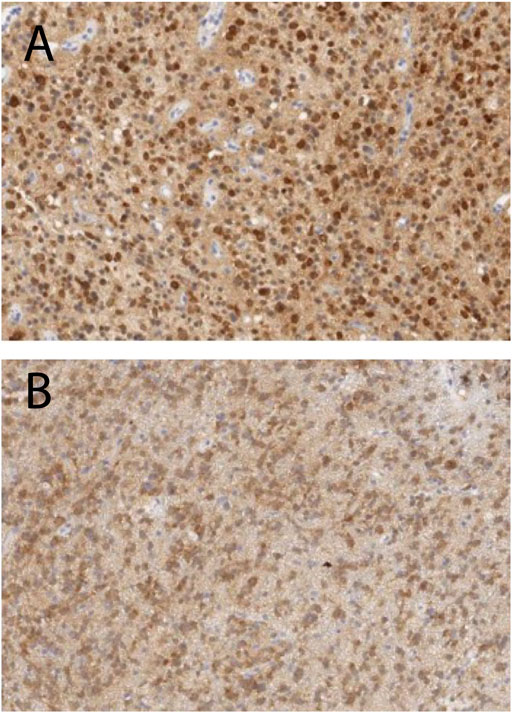
FIGURE 7. Histopathologic correlation from Type B tissue in Patient 1 (grade 3 glioma) and Type A tissue in Patient 2 (grade 2 glioma), stained for IDH-R132H and demonstrating densely cellular solid tumor in Patient 1 (A) and less dense and diffusely infiltrating tumor cells in Patient 2 (B).
Clinical dMRI typically uses 1–2 b-values to obtain average diffusion properties (e.g. mean diffusivity, fractional anisotropy and kurtosis) of tissues and is not able to capture the large range of diffusion tensors necessary to describe the complexity and heterogeneity of biologic tissues. The high b-values (up to 17,800 s/mm2) and short echo time achieved by the Connectome scanner provide a unique approach for improved characterization of tissue microstructure in a global and non-invasive fashion. We show that the multi-shell DTI data acquired on the Connectome allow us to perform analysis of a full diffusion tensor distribution in a healthy subject and patients with diffuse gliomas. Our results suggest the presence of a significant amount of signals associated with planar characters of the diffusion tensors (both with and without axial symmetry).
Given the ill-conditioned nature of the exponential kernel, it is desirable to examine the uncertainty of the inversion results. Figures 8, 9 show our preliminary uncertainty analysis on a few voxels for the healthy subject and the glioma Patient 1. For each voxel, we created 100 realizations of the data points by adding Gaussian noises to the fit from the FDTD analysis. The noise amplitude is determined from the experimental data. The obtained 100 realizations are further analyzed by FDTD to determine the average and standard deviation of Wiso, Wdisc, Wneedle, Wani−disk and Wani−3D, shown in panels (C) of Figures 8, 9. It is clear that the observed variance is quite small for all voxels.
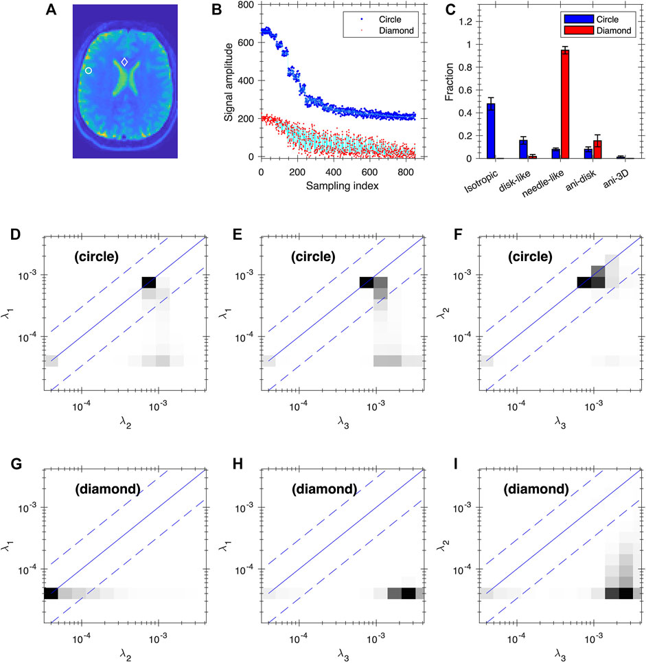
FIGURE 8. Uncertainty analysis at two voxels of the healthy subject. Panel (A) shows the positions of the two voxels (circle and diamond, same voxels as in Figure 3B1–4). (B) Plot of the data points (blue and red dots) and fitting (cyan lines) based on FDTD analysis for the two voxels. The blue data points and the corresponding fit are shifted up by 200 for clarity. (C) The average and standard deviation of Wiso, Wdisc, and Wneedle, Wani−disk and Wani−3D. Panels (D–F) and (G–I) are the average 2D projections of FDTD at the circle and diamond voxels, respectively. The projections are shown as grey map from zero to the maximum of each plot.

FIGURE 9. Uncertainty analysis at two voxels of the glioma Patient 1. (A) The two voxels mark the center (circle) and peripheral (diamond) regions of the tumor. (B) Plot of the data points (blue and red dots) and fitting (cyan lines) based on FDTD analysis for the two voxels. The blue data points and the corresponding fit are shifted up by 200 for clarity. (C) The average and standard deviation of Wiso, Wdisc, and Wneedle, Wani−disk and Wani−3D. Panels (D–F) and (G–I) are the average 2D projections of FDTD at the circle and diamond voxels, respectively. The projections are shown as grey map from zero to the maximum of each plot.
The observation of signals associated with the planar characters of the diffusion tensor is quite different from the conventional assumption of many dMRI models, such as NODDI [19] and AxCaliber [62] in that only isotropic and prolate tensors are considered. On the other hand, Wedeen et al. [63] suggested that the 2D sheet structure is common “throughout cerebral white matter and in all species, orientations, and curvatures”. Planar symmetry in diffusion tensor was found in epidermoid cysts but also for normal brain tissues with a weaker but finite planar anisotropy [64]. Laminar structure has also been reported in the cortical regions using polarization-sensitive OCT down to a spatial resolution of 4–10 μm [65]. Recently, Lichtman’s group has reported electron microscopy imaging of brain tissues by identifying cells down to 4 nm resolution and showed layered structures in the cortex with distinct cell types, cell body sizes, and orientations [66]. Mechanical stress in tumors has been shown to cause cellular deformation along the plane between solid tumor normal tissue [67] and may be a possible source of planar tissue signatures. Given such a complex structure of brain tissues, we would expect that the assumption of only isotropic and prolate tensors would be considered a simplified model and thus oblate tensors and of other symmetries should be considered. In addition, our model may be also viewed as a useful numerical representation of the diffusion data that is amenable to data-driven analysis such as K-means clustering.
The FDTD data and the associated K-means analysis in subjects with diffuse gliomas demonstrates areas of tissue heterogeneity within the tumor ROI that are not evident on conventional T2/FLAIR sequences. The different distribution of Type A (corresponding to c3 from the K-means analysis) and Type B tissue (corresponding to c4 and c5 from the K-means analysis) between the two glioma patients may be related to the degree of tumor cellularity, given that, histologically, Type B tissue in Patient 1 corresponded to areas of densely cellular solid tumor (which is expected in a grade 3 glioma). By contrast, in Patient 2, Type A tissue corresponded to moderately cellular infiltrating tumor cells as is expected in a grade 2 glioma. Further histopathologic correlation and characterization of dMRI characteristics in additional subjects is ongoing.
It is interesting to visualize how the K-means method classifies the diffusion tensors and thus differentiate the tissues. Figure 10 shows a 3D plot of the three components: Wiso, Wdisc, and Wneedle for isotropic, disc-like, and needle-like water signals respectively. Each cluster is identified by a different color and symbol. As shown in Figure 10, the clusters occupy distinct regions in this space, indicating that the three parameters (Wiso, Wdisc, and Wneedle) reflect different tissue compartments. For example, c5 is characterized by primarily high Wiso signal and low on other signals, Wdisc, and Wneedle. Furthermore, the clusters appear to overlap with each other to varying degrees, thus suggesting that there can be some uncertainties in the assignment of the clusters.
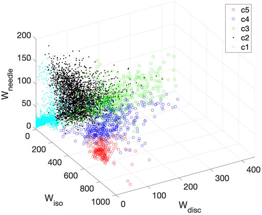
FIGURE 10. 3D plot of all clusters derived for Patient 1 in the space of Wiso, Wdisc, and Wneedle. Each cluster is represented by a different color symbol. The clusters occupy largely distinct regions in this space.
Previous Connectome dMRI data were used to probe the time dependence in diffusion coefficient typically with many more scans/diffusion times [34], and averaging the signals with all gradient directions orthogonal to the fiber direction [34, 39]. In the current work, the full angular dependence of the signal was preserved, and we found that the signals with the two diffusion times are consistent with a FDTD independent of the diffusion time within the noises. The direct benefit of the two diffusion times is the resulting high maximum b value.
Recognizing that our multi-shell DTI experiments were performed on a highly specialized and not commercially accessible MRI scanner, it is, however, conceivable that the range of b values may be achieved on select clinical scanners for certain applications. For example, our data in glioma patients could theoretically be obtained with a maximum b-value of 6,000 s/mm2. While this b value may not optimally probe specific structures such as axon diameter, it might be sufficient to identify tissue heterogeneity within diffuse gliomas. Future work will focus on implementing a similar acquisition protocol on the Siemens Prisma scanner which is equipped with 80 mT/m gradients, which is higher than gradients on conventional clinical MRI scanners.
The main disadvantage of a multi-shell protocol is the long data acquisition time. The current protocol using a standard approach for both angular and b value sampling was about 60 min in duration. Optimization of the sampling pattern can be studied with a goal to accelerate the measurement. For example, since most of the angular information is from the high b-value data, angular sampling can be reduced for low b values. Also, the distribution of b-shells can be adjusted to match the relevant range of diffusion coefficients. A recent method to optimize sampling pattern of similar experiments [68] can be performed to systematically explore different sampling patterns with an explicit optimization goal of acceleration. The unique properties of the Connectome scanner, combined with our FDTD analysis approach, can be leveraged to improve our understanding of tissue microstructure in healthy and diseased brain tissue. Ultimately, this knowledge can be used to develop and optimize protocols for clinical scanners which are sensitive to the underlying tissue biology that is being studied.
Other techniques with more complex field gradients have been developed for characterizing microscopic diffusion anisotropy using double-PFG sequence [69–72] and recently summarized Double Diffusion Encoding (DDE) approaches [73]. These sequences are designed to sensitize diffusion tensor anisotropy and tensor orientation differently by employing more complex gradient modulation sequences [1, 74–76]. These novel sequences and methods represent a significant progress in our understanding of diffusion in complex tissue structures and could help resolve uncertainties that arise due to limitations of single diffusion-encoding methods and FDTD analysis (and DTD in general) such as the lack of explicit time-dependence of diffusion [34, 39] and exchanges between compartments (see review Ref. [72]). On the other hand, the DDE and related experiments (such as QTI [76]) require complex gradient modulations resulting in longer gradient pulses and thus a reduced SNR. It would be exciting to conduct DDE/QTI experiments on the Connectome scanner [77] and analyze the results with FDTD to fully evaluate their potential [5] in vivo and possibly in combination with relaxation measurements [78–84].
This paper demonstrates the feasibility of the FDTD approach to analyze in vivo multi-shell DTI data obtained from the Connectome scanner. In contrast to many prior works on dMRI, we approached the analysis of dMRI data from a unconstraint diffusion tensor perspective to reduce human bias and oversimplification of underlying tissue microstructure. We significantly expanded the range of diffusion tensor without constraint on the form of distribution in the data inversion and used a data-centric method K-means to classify the diffusion properties of tissues. We show that the FDTD-K-means approach yields promising results of automated tissue classification in subjects with diffuse gliomas. Further validation of this approach in a larger patient cohort is underway.
The original contributions presented in the study are included in the article/Supplementary Materials, further inquiries can be directed to the corresponding author.
The studies involving human participants were reviewed and approved by the Partners Institutional Review Board, Massachusetts General Hospital. The patients/participants provided their written informed consent to participate in this study.
YS, IL, SH, BR, and EG conceived the project and wrote the paper, IL and QF collected the data, YS, IL, SH, EG, and QF performed data analysis, AN contributed to the design of experiments, MM performed histopathologic correlation of imaging findings, WC performed tissue acquisition, and IL, SYH, JD and DAF contributed to subject recruitment.
This study was supported by the National Institutes of Health (grant numbers P41-EB017183, P41-EB030006, U01-EB026996, K12CA090354, K23-NS096056, and R01-NS118187).
The authors declare that the research was conducted in the absence of any commercial or financial relationships that could be construed as a potential conflict of interest.
All claims expressed in this article are solely those of the authors and do not necessarily represent those of their affiliated organizations, or those of the publisher, the editors and the reviewers. Any product that may be evaluated in this article, or claim that may be made by its manufacturer, is not guaranteed or endorsed by the publisher.
We thank Dr. Barbara Wichtmann for helpful discussions and Dr. Qiyuan Tian for assistance in data processing.
1. Alexander DC, Dyrby TB, Nilsson M, Zhang H. Imaging Brain Microstructure with Diffusion MRI: Practicality and Applications. NMR Biomed (2019) 32:e3841. doi:10.1002/nbm.3841
2. Topgaard D. Diffusion Tensor Distribution Imaging. NMR Biomed (2019) 32:e4066–12. doi:10.1002/nbm.4066
3. Novikov DS, Fieremans E, Jespersen SN, Kiselev VG. Quantifying Brain Microstructure with Diffusion MRI: Theory and Parameter Estimation. NMR Biomed (2019) 32:e3998. doi:10.1002/nbm.3998
4. Assaf Y, Johansen‐Berg H, Thiebaut de Schotten M. The Role of Diffusion MRI in Neuroscience. NMR Biomed (2019) 32:e3762. doi:10.1002/nbm.3762
5. Huang SY, Witzel T, Keil B, Scholz A, Davids M, Dietz P, et al. Connectome 2.0: Developing the Next-Generation Ultra-high Gradient Strength Human MRI Scanner for Bridging Studies of the Micro-, Meso- and Macro-Connectome. NeuroImage (2021) 243:118530. doi:10.1016/j.neuroimage.2021.118530
6. Basser PJ, Mattiello J, LeBihan D. MR Diffusion Tensor Spectroscopy and Imaging. Biophysical J (1994) 66:259–67. doi:10.1016/s0006-3495(94)80775-1
7. Pierpaoli C, Jezzard P, Basser PJ, Barnett A, Di Chiro G. Diffusion Tensor MR Imaging of the Human Brain. Radiology (1996) 201:637–48. doi:10.1148/radiology.201.3.8939209
8. Basser PJ, Pajevic S, Pierpaoli C, Duda J, Aldroubi A. In Vivo fiber Tractography Using DT-MRI Data. Magn Reson Med (2000) 44:625–32. doi:10.1002/1522-2594(200010)44:4<625::aid-mrm17>3.0.co;2-o
9. Kenkel D, von Spiczak J, Wurnig MC, Filli L, Steidle G, Wyss M, et al. Whole-Body Diffusion Tensor Imaging. J Comput Assist Tomography (2016) 40:183–8. doi:10.1097/rct.0000000000000324
10. Jiang L, Xiao C-Y, Xu Q, Sun J, Chen H, Chen Y-C, et al. Analysis of DTI-Derived Tensor Metrics in Differential Diagnosis between Low-Grade and High-Grade Gliomas. Front Aging Neurosci (2017) 9:271. doi:10.3389/fnagi.2017.00271
11. Xu J, Humphrey PA, Kibel AS, Snyder AZ, Narra VR, Ackerman JJH, et al. Magnetic Resonance Diffusion Characteristics of Histologically Defined Prostate Cancer in Humans. Magn Reson Med (2009) 61:842–50. doi:10.1002/mrm.21896
12. Gholizadeh N, Greer PB, Simpson J, Denham J, Lau P, Dowling J, et al. Characterization of Prostate Cancer Using Diffusion Tensor Imaging: A New Perspective. Eur J Radiol (2019) 110:112–20. doi:10.1016/j.ejrad.2018.11.026
13. White NS, McDonald CR, Farid N, Kuperman J, Karow D, Schenker-Ahmed NM, et al. Diffusion-Weighted Imaging in Cancer: Physical Foundations and Applications of Restriction Spectrum Imaging. Cancer Res (2014) 74:4638–52. doi:10.1158/0008-5472.can-13-3534
14. Alexander AL, Hasan KM, Lazar M, Tsuruda JS, Parker DL. Analysis of Partial Volume Effects in Diffusion-Tensor MRI. Magn Reson Med (2001) 45:770–80. doi:10.1002/mrm.1105
15. Tuch DS, Reese TG, Wiegell MR, Makris N, Belliveau JW, Wedeen VJ. High Angular Resolution Diffusion Imaging Reveals Intravoxel white Matter Fiber Heterogeneity. Magn Reson Med (2002) 48:577–82. doi:10.1002/mrm.10268
16. Jespersen SN, Kroenke CD, Østergaard L, Ackerman JJH, Yablonskiy DA. Modeling Dendrite Density from Magnetic Resonance Diffusion Measurements. NeuroImage (2007) 34:1473–86. doi:10.1016/j.neuroimage.2006.10.037
17. Pasternak O, Sochen N, Gur Y, Intrator N, Assaf Y. Free Water Elimination and Mapping from Diffusion MRI. Magn Reson Med (2009) 62:717–30. doi:10.1002/mrm.22055
18. Metzler-Baddeley C, O'Sullivan MJ, Bells S, Pasternak O, Jones DK. How and How Not to Correct for CSF-Contamination in Diffusion MRI. NeuroImage (2012) 59:1394–403. doi:10.1016/j.neuroimage.2011.08.043
19. Zhang H, Schneider T, Wheeler-Kingshott CA, Alexander DC. NODDI: Practical In Vivo Neurite Orientation Dispersion and Density Imaging of the Human Brain. NeuroImage (2012) 61:1000–16. doi:10.1016/j.neuroimage.2012.03.072
20. Vangelderen P, Despres D, Vanzijl PCM, Moonen CTW. Evaluation of Restricted Diffusion in Cylinders. Phosphocreatine in Rabbit Leg Muscle. J Magn Reson Ser B (1994) 103:255–60. doi:10.1006/jmrb.1994.1038
21. White NS, Leergaard TB, D'Arceuil H, Bjaalie JG, Dale AM. Probing Tissue Microstructure with Restriction Spectrum Imaging: Histological and Theoretical Validation. Hum Brain Mapp (2013) 34:327–46. doi:10.1002/hbm.21454
22. Mitchell J, Chandrasekera TC, Gladden LF. Numerical Estimation of Relaxation and Diffusion Distributions in Two Dimensions. Prog Nucl Magn Reson Spectrosc (2011) 62:34–50. doi:10.1016/j.pnmrs.2011.07.002
23. Jian B, Vemuri BC, Özarslan E, Carney PR, Mareci TH. A Novel Tensor Distribution Model for the Diffusion-Weighted MR Signal. NeuroImage (2007) 37:164–76. doi:10.1016/j.neuroimage.2007.03.074
24. Lampinen B, Szczepankiewicz F, Mårtensson J, van Westen D, Sundgren PC, Nilsson M. Neurite Density Imaging versus Imaging of Microscopic Anisotropy in Diffusion MRI: A Model Comparison Using Spherical Tensor Encoding. NeuroImage (2017) 147:517–31. doi:10.1016/j.neuroimage.2016.11.053
25. Palombo M, Ianus A, Guerreri M, Nunes D, Alexander DC, Shemesh N, et al. SANDI: A Compartment-Based Model for Non-invasive Apparent Soma and Neurite Imaging by Diffusion MRI. Neuroimage (2020) 215:116835. doi:10.1016/j.neuroimage.2020.116835
26. Yablonskiy DA, Bretthorst GL, Ackerman JJH. Statistical Model for Diffusion Attenuated MR Signal. Magn Reson Med (2003) 50:664–9. doi:10.1002/mrm.10578
27. Basser PJ, Pajevic S. A Normal Distribution for Tensor-Valued Random Variables: Applications to Diffusion Tensor Mri. IEEE Trans Med Imaging (2003) 22:785–94. doi:10.1109/tmi.2003.815059
28. Scherrer B, Schwartzman A, Taquet M, Sahin M, Prabhu SP, Warfield SK. Characterizing Brain Tissue by Assessment of the Distribution of Anisotropic Microstructural Environments in Diffusion-Compartment Imaging (DIAMOND). Magn Reson Med (2016) 76:963–77. doi:10.1002/mrm.25912
29. Magdoom KN, Pajevic S, Dario G, Basser PJ. A New Framework for MR Diffusion Tensor Distribution. Sci Rep (2021) 11:2766. doi:10.1038/s41598-021-81264-x
30. Jelescu IO, Veraart J, Fieremans E, Novikov DS. Degeneracy in Model Parameter Estimation for Multi-Compartmental Diffusion in Neuronal Tissue. NMR Biomed (2016) 29:33–47. doi:10.1002/nbm.3450
31. Henriques RN, Jespersen SN, Shemesh N. Microscopic Anisotropy Misestimation in Spherical-Mean Single Diffusion Encoding MRI. Magn Reson Med (2019) 81:3245–61. doi:10.1002/mrm.27606
32. Setsompop K, Kimmlingen R, Eberlein E, Witzel T, Cohen-Adad J, McNab JA, et al. Pushing the Limits of In Vivo Diffusion MRI for the Human Connectome Project. NeuroImage (2013) 80:220–33. doi:10.1016/j.neuroimage.2013.05.078
33. McNab JA, Edlow BL, Witzel T, Huang SY, Bhat H, Heberlein K, et al. The Human Connectome Project and beyond: Initial Applications of 300mT/m Gradients. NeuroImage (2013) 80:234–45. doi:10.1016/j.neuroimage.2013.05.074
34. Huang SY, Nummenmaa A, Witzel T, Duval T, Cohen-Adad J, Wald LL, et al. The Impact of Gradient Strength on In Vivo Diffusion MRI Estimates of Axon Diameter. NeuroImage (2015) 106:464–72. doi:10.1016/j.neuroimage.2014.12.008
35. Fan Q, Nummenmaa A, Witzel T, Zanzonico R, Keil B, Cauley S, et al. Investigating the Capability to Resolve Complex White Matter Structures with High B-Value Diffusion Magnetic Resonance Imaging on the MGH-USC Connectom Scanner. Brain Connectivity (2014) 4:718–26. doi:10.1089/brain.2014.0305
36. Bishop CM. Pattern Recognition and Machine Learning. New York: Springer Science+Business Media, LLC (2006).
37. Fan Q, Tian Q, Ohringer NA, Nummenmaa A, Witzel T, Tobyne SM, et al. Age-related Alterations in Axonal Microstructure in the Corpus Callosum Measured by High-Gradient Diffusion MRI. NeuroImage (2019) 191:325–36. doi:10.1016/j.neuroimage.2019.02.036
38. Huang SY, Fan Q, Machado N, Eloyan A, Bireley JD, Russo AW, et al. Corpus Callosum Axon Diameter Relates to Cognitive Impairment in Multiple Sclerosis. Ann Clin Transl Neurol (2019) 6:882–92. doi:10.1002/acn3.760
39. Huang SY, Tian Q, Fan Q, Witzel T, Wichtmann B, McNab JA, et al. High-gradient Diffusion MRI Reveals Distinct Estimates of Axon Diameter index within Different white Matter Tracts in the In Vivo Human Brain. Brain Struct Funct (2020) 225:1277–91. doi:10.1007/s00429-019-01961-2
40. Herberthson M, Yolcu C, Knutsson H, Westin C-F, Özarslan E. Orientationally-averaged Diffusion-Attenuated Magnetic Resonance Signal for Locally-Anisotropic Diffusion. Sci Rep (2019) 9:4899. doi:10.1038/s41598-019-41317-8
42. Jensen JH, Helpern JA, Ramani A, Lu H, Kaczynski K. Diffusional Kurtosis Imaging: The Quantification of Non-gaussian Water Diffusion by Means of Magnetic Resonance Imaging. Magn Reson Med (2005) 53:1432–40. doi:10.1002/mrm.20508
43. Keil B, Blau JN, Biber S, Hoecht P, Tountcheva V, Setsompop K, et al. A 64-channel 3T Array Coil for Accelerated Brain MRI. Magn Reson Med (2013) 70:248–58. doi:10.1002/mrm.24427
44. Provencher SW. Contin: A General Purpose Constrained Regularization Program for Inverting Noisy Linear Algebraic and Integral Equations. Comput Phys Commun (1982) 27:229–42. doi:10.1016/0010-4655(82)90174-6
45. Song Y-Q, Venkataramanan L, Hürlimann MD, Flaum M, Frulla P, Straley C. T1-T2 Correlation Spectra Obtained Using a Fast Two-Dimensional Laplace Inversion. J Magn Reson (2002) 154:261–8. doi:10.1006/jmre.2001.2474
46. Venkataramanan L, Yi-Qiao Song YQ, Hürlimann MD. Solving Fredholm Integrals of the First Kind with Tensor Product Structure in 2 and 2.5 Dimensions. IEEE Trans Signal Process (2002) 50:1017–26. doi:10.1109/78.995059
47. Baglama J, Reichel L. Augmented Implicitly Restarted Lanczos Bidiagonalization Methods. SIAM J Sci Comput (2005) 27:19–42. doi:10.1137/04060593x
48. Budde MD, Frank JA. Neurite Beading Is Sufficient to Decrease the Apparent Diffusion Coefficient after Ischemic Stroke. Proc Natl Acad Sci U.S.A (2010) 107:14472–7. doi:10.1073/pnas.1004841107
49. Song Y-Q, Venkataramanan L, Burcaw L. Determining the Resolution of Laplace Inversion Spectrum. J Chem Phys (2005) 122:104104. doi:10.1063/1.1858436
50. de Almeida Martins JP, Topgaard D. Multidimensional Correlation of Nuclear Relaxation Rates and Diffusion Tensors for Model-free Investigations of Heterogeneous Anisotropic Porous Materials. Sci Rep (2018) 8:2488. doi:10.1038/s41598-018-19826-9
51. Parker RL, Song Y-Q. Assigning Uncertainties in the Inversion of NMR Relaxation Data. J Magn Reson (2005) 174:314–24. doi:10.1016/j.jmr.2005.03.002
52. Song Y-Q. Resolution and Uncertainty of Laplace Inversion Spectrum. Magn Reson Imaging (2007) 25:445–8. doi:10.1016/j.mri.2006.11.023
53. Prange M, Song Y-Q. Quantifying Uncertainty in NMR Spectra Using Monte Carlo Inversion. J Magn Reson (2009) 196:54–60. doi:10.1016/j.jmr.2008.10.008
54. Louis DN, Perry A, Wesseling P, Brat DJ, Cree IA, Figarella-Branger D, et al. The 2021 WHO Classification of Tumors of the Central Nervous System: a Summary. Neuro-Oncology (2021) 23:1231–51. doi:10.1093/neuonc/noab106
55. Buckner JC, Shaw EG, Pugh SL, Chakravarti A, Gilbert MR, Barger GR, et al. Radiation Plus Procarbazine, CCNU, and Vincristine in Low-Grade Glioma. N Engl J Med (2016) 374:1344–55. doi:10.1056/nejmoa1500925
56. Stupp R, Mason WP, van den Bent MJ, Weller M, Fisher B, Taphoorn MJB, et al. Radiotherapy Plus Concomitant and Adjuvant Temozolomide for Glioblastoma. N Engl J Med (2005) 352:987–96. doi:10.1056/nejmoa043330
57. Parsons DW, Jones S, Zhang X, Lin JC-H, Leary RJ, Angenendt P, et al. An Integrated Genomic Analysis of Human Glioblastoma Multiforme. Science (2008) 321:1807–12. doi:10.1126/science.1164382
58. Yan H, Parsons DW, Jin G, McLendon R, Rasheed BA, Yuan W, et al. IDH1andIDH2Mutations in Gliomas. N Engl J Med (2009) 360:765–73. doi:10.1056/nejmoa0808710
59. van den Bent MJ, Dubbink HJ, Marie Y, Brandes AA, Taphoorn MJB, Wesseling P, et al. IDH1 and IDH2 Mutations Are Prognostic but Not Predictive for Outcome in Anaplastic Oligodendroglial Tumors: A Report of the European Organization for Research and Treatment of Cancer Brain Tumor Group. Clin Cancer Res (2010) 16:1597–604. doi:10.1158/1078-0432.ccr-09-2902
60. Hartmann C, Hentschel B, Wick W, Capper D, Felsberg J, Simon M, et al. Patients with IDH1 Wild Type Anaplastic Astrocytomas Exhibit Worse Prognosis Than IDH1-Mutated Glioblastomas, and IDH1 Mutation Status Accounts for the Unfavorable Prognostic Effect of Higher Age: Implications for Classification of Gliomas. Acta Neuropathol (2010) 120:707–18. doi:10.1007/s00401-010-0781-z
61. Stadlbauer A, Buchfelder M, Salomonowitz E, Ganslandt O. Fiber Density Mapping of Gliomas: Histopathologic Evaluation of a Diffusion-Tensor Imaging Data Processing Method. Radiology (2010) 257:846–53. doi:10.1148/radiol.10100343
62. Assaf Y, Blumenfeld-Katzir T, Yovel Y, Basser PJ. Axcaliber: A Method for Measuring Axon Diameter Distribution from Diffusion MRI. Magn Reson Med (2008) 59:1347–54. doi:10.1002/mrm.21577
63. Wedeen VJ, Rosene DL, Wang R, Dai G, Mortazavi F, Hagmann P, et al. The Geometric Structure of the Brain Fiber Pathways. Science (2012) 335:1628–34. doi:10.1126/science.1215280
64. Santhosh K, Thomas B, Radhakrishnan VV, Saini J, Kesavadas C, Gupta AK, et al. Diffusion Tensor and Tensor Metrics Imaging in Intracranial Epidermoid Cysts. J Magn Reson Imaging (2009) 29:967–70. doi:10.1002/jmri.21686
65. Liu CJ, Ammon W, Jones RJ, Nolan J, Wang R, Chang S, et al. Refractive-index Matching Enhanced Polarization Sensitive Optical Coherence Tomography Quantification in Human Brain Tissue. Biomed Opt Express (2021) 13:358. doi:10.1364/boe.443066
66. Shapson-Coe A, Januszewski M, Berger DR, Pope A, Wu Y, Blakely T, et al. A Connectomic Study of a Petascale Fragment of Human Cerebral Cortex. bioRxiv (2021):1–59. doi:10.1101/2021.05.29.446289
67. Seano G, Nia HT, Emblem KE, Datta M, Ren J, Krishnan S, et al. Solid Stress in Brain Tumours Causes Neuronal Loss and Neurological Dysfunction and Can Be Reversed by Lithium. Nat Biomed Eng (2019) 3:230–45. doi:10.1038/s41551-018-0334-7
68. Song YQ, Xiao L. Optimization of Multidimensional MR Data Acquisition for Relaxation and Diffusion. NMR Biomed (2020) 33:e4238. doi:10.1002/nbm.4238
69. Mitra PP. Multiple Wave-Vector Extensions of the NMR Pulsed-Field-Gradient Spin-echo Diffusion Measurement. Phys Rev B (1995) 51:15074–8. doi:10.1103/physrevb.51.15074
70. Cheng Y, Cory DG. Multiple Scattering by NMR. J Am Chem Soc (1999) 121:7935–6. doi:10.1021/ja9843324
71. Ianuş A, Jespersen SN, Serradas Duarte T, Alexander DC, Drobnjak I, Shemesh N. Accurate Estimation of Microscopic Diffusion Anisotropy and its Time Dependence in the Mouse Brain. NeuroImage (2018) 183:934–49. doi:10.1016/j.neuroimage.2018.08.034
72. Henriques RN, Palombo M, Jespersen SN, Shemesh N, Lundell H, Ianuş A. Double Diffusion Encoding and Applications for Biomedical Imaging. J Neurosci Methods (2021) 348:108989. doi:10.1016/j.jneumeth.2020.108989
73. Shemesh N, Jespersen SN, Alexander DC, Cohen Y, Drobnjak I, Dyrby TB, et al. Conventions and Nomenclature for Double Diffusion Encoding NMR and MRI. Magn Reson Med (2016) 75:82–7. doi:10.1002/mrm.25901
74. de Almeida Martins JP, Topgaard D. Two-dimensional Correlation of Isotropic and Directional Diffusion Using NMR. Phys Rev Lett (2016) 116:087601. doi:10.1103/PhysRevLett.116.087601
75. Szczepankiewicz F, Lasič S, van Westen D, Sundgren PC, Englund E, Westin C-F, et al. Quantification of Microscopic Diffusion Anisotropy Disentangles Effects of Orientation Dispersion from Microstructure: Applications in Healthy Volunteers and in Brain Tumors. NeuroImage (2015) 104:241–52. doi:10.1016/j.neuroimage.2014.09.057
76. Westin C-F, Knutsson H, Pasternak O, Szczepankiewicz F, Özarslan E, van Westen D, et al. Q-space Trajectory Imaging for Multidimensional Diffusion MRI of the Human Brain. NeuroImage (2016) 135:345–62. doi:10.1016/j.neuroimage.2016.02.039
77. Nilsson M, Larsson J, Lundberg D, Szczepankiewicz F, Witzel T, Westin C-F, et al. Liquid crystal Phantom for Validation of Microscopic Diffusion Anisotropy Measurements on Clinical MRI Systems. Magn Reson Med (2018) 79:1817–28. doi:10.1002/mrm.26814
78. de Almeida Martins JP, Tax CMW, Szczepankiewicz F, Jones DK, Westin C-F, Topgaard D. Transferring Principles of Solid-State and Laplace NMR to the Field of In Vivo Brain MRI. Magn Reson (2020) 1:27–43. doi:10.5194/mr-1-27-2020
79. Naranjo ID, Reymbaut A, Brynolfsson P, Lo Gullo R, Bryskhe K, Topgaard D, et al. Multidimensional Diffusion Magnetic Resonance Imaging for Characterization of Tissue Microstructure in Breast Cancer Patients: A Prospective Pilot Study. Cancers (2021) 13:1606. doi:10.3390/cancers13071606
80. Martin J, Reymbaut A, Schmidt M, Doerfler A, Uder M, Laun FB, et al. Nonparametric D-R1-R2 Distribution MRI of the Living Human Brain. NeuroImage (2021) 245:118753. doi:10.1016/j.neuroimage.2021.118753
81. Reymbaut A, Critchley J, Durighel G, Sprenger T, Sughrue M, Bryskhe K, et al. Toward Nonparametric Diffusion‐ Characterization of Crossing Fibers in the Human Brain. Magn Reson Med (2021) 85:2815–27. doi:10.1002/mrm.28604
82. Benjamini D, Basser PJ. Multidimensional Correlation MRI. NMR Biomed (2020) 33:e4226. doi:10.1002/nbm.4226
83. Hutter J, Slator PJ, Christiaens D, Teixeira RPAG, Roberts T, Jackson L, et al. Integrated and Efficient Diffusion-Relaxometry Using ZEBRA. Sci Rep (2018) 8:15138. doi:10.1038/s41598-018-33463-2
Keywords: magnetic resonance imaging, connectome scanner, diffusion tensor imaging, glioma tumor, full diffusion tensor distribution
Citation: Song Y, Ly I, Fan Q, Nummenmaa A, Martinez-Lage M, Curry WT, Dietrich J, Forst DA, Rosen BR, Huang SY and Gerstner ER (2022) Measurement of Full Diffusion Tensor Distribution Using High-Gradient Diffusion MRI and Applications in Diffuse Gliomas. Front. Phys. 10:813475. doi: 10.3389/fphy.2022.813475
Received: 11 November 2021; Accepted: 23 February 2022;
Published: 12 April 2022.
Edited by:
Dan Benjamini, National Institute on Aging (NIH), United StatesReviewed by:
Andrada Ianus, Champalimaud Foundation, PortugalCopyright © 2022 Song, Ly, Fan, Nummenmaa, Martinez-Lage, Curry, Dietrich, Forst, Rosen, Huang and Gerstner. This is an open-access article distributed under the terms of the Creative Commons Attribution License (CC BY). The use, distribution or reproduction in other forums is permitted, provided the original author(s) and the copyright owner(s) are credited and that the original publication in this journal is cited, in accordance with accepted academic practice. No use, distribution or reproduction is permitted which does not comply with these terms.
*Correspondence: Yiqiao Song, eXNvbmc1QG1naC5oYXJ2YXJkLmVkdQ==
Disclaimer: All claims expressed in this article are solely those of the authors and do not necessarily represent those of their affiliated organizations, or those of the publisher, the editors and the reviewers. Any product that may be evaluated in this article or claim that may be made by its manufacturer is not guaranteed or endorsed by the publisher.
Research integrity at Frontiers
Learn more about the work of our research integrity team to safeguard the quality of each article we publish.