Novel Numerical Method Based on the Analog Equation Method for a Class of Anisotropic Convection-Diffusion Problems

In this work, a CMFS method based on the analogy equation method, the radial basis function and the method of fundamental solutions for linear and nonlinear convection-diffusion equations in anisotropic materials is presented. The analog equation method is utilized to transform the linear and nonlinear convection-diffusion equation into an equivalent one. The expressions of the homogeneous solution and particular solution are derived by utilizing the radial basis function approximation and the method of fundamental solutions, respectively. By enforcing the desired solution to satisfy the original convection-diffusion equation with boundary conditions at boundary and internal collocation points yield a nonlinear system of equations, which can be solved by using the Newton-Raphson iteration or the Picard method of iteration. The error convergence curves of the proposed meshless method have been investigated by using different globally supported radial basis functions. Numerical experiments show that the proposed CMFS method is promising for anisotropic convection-diffusion problems with accurate and stable results.

1 Introduction

Partial differential equations (PDEs) are generally utilized in understanding and modeling of a considerable lot of realism matters show up in applied science and material science. The PDE models are utilized in numerous fields, for example, plasma physics, hydrodynamics, finance, biology and nonlinear optic [1–3]. It is pointed that it is hard to tackle nonlinear problems most of the cases, especially analytically. Numerous strategies have been developed by the researchers for the numerical solution of complex problems (see [4–6] and the references therein). Among these techniques, one of the most attractive group of techniques is radial basis function (RBF) based techniques.

The RBF techniques are attractive in numerical simulation thanks to their simple, flexible, and truly meshfree features. These techniques have been successfully applied to diverse problems in a simple-to-implement fashion. The popular RBF-based numerical methods include the Kansa’s method [7, 8], the method of fundamental solution (MFS) [9–12], the boundary knot method [13–15], the modified method of fundamental solutions [16–18] which have been well-developed and applied to a variety of boundary value problems.

In previous literatures, the polynomial RBFs, thin plate spline, Gaussians, and Multiquadrics are often used [19–21]. It is noted that the traditional RBF-based schemes are indirect and global in the sense that the expansion coefficients are used as the basic variables in the numerical solution procedure, while the global RBF interpolation leads to the full matrix. Roughly speaking, the RBF-based approaches can be classified as two types. The first category uses RBFs to approximate the particular solution of a partial differential equation (PDE) of interest, and the homogeneous part is obtained by means of numerical methods, like the boundary element method, the MFS, or the boundary knot method. The second category is the domain-type collocation methods. According to this approach, the RBF expansion is utilized directly for the unknown solution, and the collocation satisfies the governing equation and boundary conditions. The Kansa’s method is a typical domain-type RBF approach. In this paper, we will develop a RBF-based technique of the first type to investigate anisotropic materials.

Anisotropic materials, characterized by varied material properties along different directions, are ubiquitous in nature and difficult to be analyzed. If non-linear property is included, the problems become even more complicated. Previously, Shin and Elman [22] studied the effect of various element discretization strategies and iteration algorithms for nonlinear convection-diffusion problems with variable velocity in isotropic materials. Torsten [23] used the anisotropic streamline-diffusion finite element method to analyze homogeneous convection-diffusion problems with dominant convection. Onyejekwe [24] applied Green element method to 2D transient convection-diffusion problems with linear reaction and variable velocity. The lattice Boltzmann method is proposed for general nonlinear anisotropic convection-diffusion equations [25,26]. The anisotropic nonlinear convection-diffusion equations are also investigated by the finite volume method [27], the finite element method [28], the finite difference method [29], the virtual element method [30]. Shang et al. [31] proposed a discrete unified gas kinetic scheme for a general nonlinear convection-diffusion equation. Cao and Zhang studied a nonlinear diffusion-convection-reaction equation with a variable coefficient which has applications in many fields [32].

Based on the above-mentioned investigations, we aim to apply the MFS, in combination with the RBF and the analog equation method (AEM) [33], to analyze anisotropic nonlinear convection-diffusion problems. First, the AEM is utilized to transform the PDE into an equivalent one. Then, the expressions of the homogeneous and particular solutions are derived by utilizing RBF approximation and the MFS, respectively. Finally, enforcing the desired solution to satisfy the original PDE with boundary conditions at boundary and internal collocation points yield a nonlinear system of equations, which can be solved by using the Newton-Raphson iteration or the Picard method of iteration. Here, we will focus on the construction of Picard method of iteration, which should be carefully constructed to reach convergence.

The structure of this paper is arranged as follows. In Section 2, we give the depiction of nonlinear convection-diffusion problems in anisotropic media. Followed in Section 3, the detailed processes are derived to construct the proposed CMFS. Numerical investigation and results analysis are carried out in Section 4. Section 5 concludes this paper and provides some comments on the CMFS.

2 Nonlinear Convection-Diffusion Problems in Anisotropic Materials

Consider an open-bounded domain $\mathrm{\Omega }\subseteq R^d,$ where $d$ represent problem’s dimension. Assuming that $\mathrm{\Omega }$ is bounded by a piecewise smooth boundary $\mathrm{\Gamma }$ which is consist of numerous sufficiently smooth segments in the Liapunov sense. The space coordinate $X\in \mathrm{\Omega }\subseteq R^d$ is utilized to denoted position of an arbitrary point. The description of convection-diffusion problems in anisotropic media can be expressed as partial differential equation

${\displaystyle \sum _{i=1}^d{\displaystyle \sum _{j=1}^d{k}_{ij}\frac{{\partial }^{2}u\left(X\right)}{\partial x_i\partial x_j}}}-\mathbf{v}\cdot \nabla u\left(X\right)=f\left(X\right)\text{,}X\in \mathrm{\Omega }(1)$

subjected to Dirichlet boundary condition

$u\left(X\right)=\overline{u}\left(X\right),X\in {\mathrm{\Gamma }}_1(\mathrm{2a})$

and Neumann boundary condition related boundary flux

$q_n\left(X\right)={\overline{q}}_n\left(X\right),X\in {\mathrm{\Gamma }}_2(\mathrm{2b})$

where $\mathbf{v}$ denotes a velocity vector and $u$ is the desired field. $\mathbf{K}=\left[k_{ij}\right]$ is the constant material tensor. Particularly, the material constant tensor for 2D cases is given by

$\mathbf{K}=\left[\begin{array}{cc}{k}_{11}& k_{12}\\ k_{12}& k_{22}\end{array}\right].$

The boundary flux is defined as $q_n=-{\displaystyle \sum _{i=1}^d{\displaystyle \sum _{j=1}^d{k}_{ij}\frac{\partial u}{\partial x_j}{n}_i}}$, where $n_i$ represent components of the unit outward normal vector $\mathbf{n}$ to the boundary $\mathrm{\Gamma }$. $f\left(X\right)$ stands for the internal forcing function, $\overline{u}$ and ${\overline{q}}_n$ are specified values on the Dirichlet and Neumann boundary, respectively. For a well-posed problem, $\mathrm{\Gamma }={\mathrm{\Gamma }}_1\cup {\mathrm{\Gamma }}_2$.

It is observed that the smaller the determinant of $\mathbf{K},$ the more asymmetric and anisotropic are the field and flux vectors, the more difficult it is to get an accurate numerical solution. Specially, if $\mathbf{K}$ is a diagonal matrix with completely equivalent diagonal elements, Eq. 1 reduces to an isotropic convection-diffusion equation. In general, when material tensor $\mathbf{K}$ or velocity vector $\mathbf{v}$ is dependent on the unknown filed $u,$ Eq. 1 shows nonlinearity. Here, we restrict our attention to research such nonlinear cases, velocity $\mathbf{v}$ is considered as a function related to the desired field u, that is, $\mathbf{v}=\mathbf{v}\left(u\right)$.

3 The CMFS Meshless Method

For the previous nonlinear problems, the proposed CMFS method is based on the combination of the AEM, globally supported RBF approximation and the MFS. Detailed processes are given below.

3.1 The Analog Equation Method

The AEM, which was improved by Burlon et al [34], was first proposed by Katsikadelis for the solution of nonlinear problems. Using the analog equation method, Eq. 1 can be converted into a Poisson type equation. Suppose $u\left(X\right)$ is the sought solution of Eq. 1, which is a continuously differentiable function with up to two orders in $\mathrm{\Omega }$. Apply the Laplacian operator to $u\left(X\right)$, we can derive

${\nabla }^{2}u=b\left(X\right).(3)$

If the source distribution $b\left(X\right)$ is known, then the solution of Eq. 1 can be produced by solving the linear Eq. 3 under the same boundary conditions (2a)-(2b), namely, Eq. 3 is equivalent to Eq. 1.

Using to the principle of superposition, the solution of linear PDE Eq. 3 can be written in the form of the sum of the particular solution $u^{\text{par}}$ and the homogeneous solution $u^{\mathrm{hom}}$, which is given as

$u=u^{\mathrm{hom}}+u^{\text{par}},(4)$

Accordingly, $u^{\mathrm{hom}}$ and $u^{\text{par}}$ should satisfy

${\nabla }^2{u}^{\text{par}}\left(X\right)=b\left(X\right)\text{,}X\in \mathrm{\Omega },(5)$

and

$\{\begin{array}{cc}{\nabla }^2{u}^{\mathrm{hom}}\left(X\right)=0,& X\in \mathrm{\Omega }\\ u^{\mathrm{hom}}\left(X\right)=\overline{u}-u^{par}\left(X\right),& X\in {\mathrm{\Gamma }}_1\\ q_n^{\mathrm{hom}}\left(X\right)={\overline{q}}_n-q_n^{par}\left(X\right),& X\in {\mathrm{\Gamma }}_2\end{array}(6)$

respectively. Furthermore, we must note that the particular solution $u^{\text{par}}$ satisfying Eq. 5 does not need to satisfy boundary conditions, so it is not unique and must be coupled with the homogeneous solution $u^{\mathrm{hom}}$ and related boundary conditions. However, our aim is just to obtain the approximating expression rather than detailed numerical methods.

3.2 Radial Basis Function Approximation to the Particular Solution

This step is to derive the particular solution by RBF approximation. There are two schemes to fulfill this procedure. The standard approach to obtain the particular solutions is to integrate an operator by means of selected RBF. This scheme is just suitable to some simple operators and RBFs which is mathematically reliable. Another approach is a reverse differential process, which has no restriction on certain operators and RBFs, but the selected RBFs must be continuously differentiable with high orders. Here, the introduction of AEM replaces the original complicated operator with a simpler Laplacian operator, so it is feasible to evaluate the particular solution using the integrating process. To this end, the fictitious term introduced in Eq. 3 can be approximated by

$b\left(X\right)={\displaystyle \sum _{m=1}^M{\alpha }_m\varphi \left(X,X_m\right)},\left(X,X_m\in \mathrm{\Omega }\right)(7)$

where $M$ is the number of interpolation points inside the domain $\mathrm{\Omega }$. ${\alpha }_j\left(j=\mathrm{1,2},\mathrm{...},M\right)$ denote coefficients to be determined, and $\varphi$ represents the radial basis function.

Similarly, it is reasonable to express the particular solution $u^{\text{par}}$ as

$u^{\text{par}}\left(X\right)={\displaystyle \sum _{m=1}^M{\alpha }_m\widehat{u}{\left(X,X\right)}_m},(8)$

if the following relationship

${\nabla }^2\widehat{u}\left(X,X_m\right)=\varphi \left(X,X_m\right),(9)$

holds, where $\widehat{u}$ is a corresponding particular basis function depending on the radial basis function $\varphi$ and can be obtained by repeated integration.

The accuracy and efficacy of the interpolation depend on the choice of the radial basis function $\varphi$, which should provide an accurate approximation to b so that Eq. 9 can be derived analytically. During the past several decades, polynomial RBFs, MQs and TPS interpolation have got hot attention from the science and engineering communities. They have been investigated for Laplacian operator in $R^2$ and $R^3$. It is noted that the MQs converge exponentially, TPS in $R^{2}O\left(h\left|\log h\right|\right)$, and traditional $1+rO\left(h^{1/2}\right)$, where $h$ is minimum separation distance [35]. As is known to all, the better the approximation properties of RBFs corresponds with the worse conditioning. For example, MQs are spectrally convergent whereas their condition number increases exponentially when the data density increases. Additionally, the selection of shape parameter in MQs is also an important factor to approximation and its small variation may cause severe differences to solutions. Thus, we consider the implementation of polynomial RBFs and MQs approximation in this paper.

3.3 The Method of Fundamental Solutions for the Homogeneous Solution

Before introducing the MFS [36, 37], it is necessary to give the definition of the fundamental solutions. The fundamental solution $u^{\ast }\left(X,Y\right)$ for the Laplacian operator is defined to satisfy

${\nabla }^2{u}^{\ast }\left(X,Y\right)+{\delta }_{XY}=0,(10)$

in an infinite domain, where ${\delta }_{XY}$ denotes the Dirac delta function which goes to infinity for the case of $X=Y$ and equals to zero elsewhere. The detailed expression of $u^{\ast }\left(X,Y\right)$ for Laplace equation is

$\{\begin{array}{l}{u}^{\ast }\left(X,Y\right)=\frac{1}{2\pi }\ln \frac{1}{r\left(X,Y\right)}\text{,}d=2\hfill \\ u^{\ast }\left(X,Y\right)=\frac{1}{4\pi r\left(X,Y\right)}\text{.}d=3\hfill \end{array}(11)$

The fundamental idea of the MFS is to place a virtual boundary outside the domain interested. Here, to obtain a weak solution of Laplace Eq. 6, collocation points $X_n\left(n=\mathrm{1,2},L\cdots ,N\right)$ and source points $Y_n\left(n=\mathrm{1,2},L\cdots ,N\right)$ are distributed on the physical boundary and the virtual boundary, respectively. Furthermore, suppose that there is a virtual source load ${\phi }_n\left(1\le n\le N\right)$ at each fictitious source point. The difference between the physical and virtual boundaries means that the homogeneous part $u^{\mathrm{hom}}$ at arbitrary field points $X$ in the domain or on the physical boundary can be constructed by a linear combination of fundamental solutions in terms of fictitious sources ${\phi }_n\left(1\le n\le N\right)$, that is,

$u^{\mathrm{hom}}\left(X\right)={\displaystyle \sum _{n=1}^N{\phi }_n{u}^{\ast }\left(X,Y_n\right)},\left(X\in \mathrm{\Omega },Y_n\in {\mathrm{\Gamma }}^{\prime }\right)(12)$

which exactly satisfies Eq. 6.

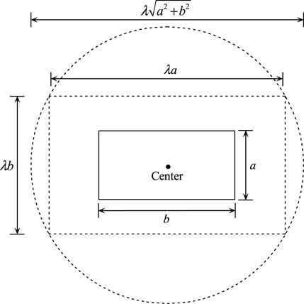
The proper usage of the MFS must concern three problems. The first case is the number of collocation points distributed on the physical boundary. However, too many collocation points may aggravate the ill-conditioned matrix. The virtual boundary shape is another important aspect. Theoretically, the virtual boundary shape can be arbitrarily chosen in the calculation. In practical computation, the virtual boundary shape is usually selected as a circle or similar shape to the actual boundary to keep algorithm versatile [38]. For example, for the rectangular domain, the rectangular or circular virtual boundaries can be used (see Figure 1).

FIGURE 1

FIGURE 1. Geometry of circular and rectangular virtual boundaries for a simple rectangular domain.

The location of the fictitious source points is also an interesting issue. It has been investigated in several literatures [39–41]. In this paper, we consider a new way to find out the proper location of the virtual boundary, a ratio parameter $\lambda$ is introduced and can be defined as follows

$\lambda =\frac{\mathrm{characteristic}\mathrm{length}\mathrm{of}\mathrm{the}\mathrm{virtual}\mathrm{boundary}}{\mathrm{characteristic}\mathrm{length}\mathrm{of}\mathrm{the}\mathrm{physical}\mathrm{boundary}}(13)$

For example, in Figure 1, if the length and height of the rectangle domain are $a$ and $b$, respectively, the location of circular and similar rectangular virtual boundary can be measured by diameter $\lambda \sqrt{a^2+b^2}$, $\lambda a$ and $\lambda b$ correspondingly. From the computation perspective, mathematical accuracy will decrease if the distance between the virtual and physical boundary turns out to be close, because of the singular disturbance of the fundamental solutions. Then again, in case when the source points are far away from the physical boundary then round-off error in floating point arithmetic may be a major issue in such case, the coefficient matrix of the system of equations is closely to zero [38]. Therefore, parameter $\lambda$ is commonly chosen to be in the range of 1.8–4.0 and 0.6–0.8 for internal and external problems respectively. Unless otherwise specified, a circular virtual boundary will be employed and parameter $\lambda =3.0$ is used to determine its location in this paper.

3.4 The Construction of Solving Equations

According to the above process, the solution $u=u\left(X\right)$ to Eq. 3 can be expressed as

$u\left(X\right)={\displaystyle \sum _{n=1}^N{\phi }_n{u}_n^{\ast }\left(X\right)}+{\displaystyle \sum _{m=1}^M{\alpha }_m{\widehat{u}}_m\left(X\right)},\left(X\in \mathrm{\Omega }\right)(14)$

which is also the solution of Eq. 1. Differentiating Eq. 14 yields

$\frac{\partial u}{\partial x_i}={\displaystyle \sum _{n=1}^N{\phi }_n\frac{\partial u_n^{\ast }\left(X\right)}{\partial x_i}}+{\displaystyle \sum _{m=1}^M{\alpha }_m\frac{\partial {\widehat{u}}_m\left(X\right)}{\partial x_i}},(15)$

$\frac{{\partial }^{2}u}{\partial x_i\partial x_j}={\displaystyle \sum _{n=1}^N{\phi }_n\frac{\partial u_n^{\ast }\left(X\right)}{\partial x_i\partial x_j}}+{\displaystyle \sum _{m=1}^M{\alpha }_m\frac{\partial {\widehat{u}}_m\left(X\right)}{\partial x_i\partial x_j}},(16)$

where $i,j=\mathrm{1,2},\mathrm{...},d$ and $u_n^{\ast }\left(X\right)=u^{\ast }\left(X,Y_n\right)$, ${\widehat{u}}_m\left(X\right)=\widehat{u}\left(X,X_m\right)$.

There are two different approaches to determine the unknowns ${\alpha }_j$ and ${\varphi }_i$ for nonlinear cases. If Eqs 14–16 directly satisfy the governing Eq. 1 at $M$ interpolation points in the domain $\mathrm{\Omega }$ and corresponding boundary conditions (2a)-(2b) at $N$ boundary collocation points, a linear or nonlinear system of $N+M$ equations can be obtained. The Newton-Raphson iteration [42] is a good choice to solve the nonlinear system. However, if we first linearize the nonlinear term, and then make Eqs. (14)-(16) satisfy Eq. (1) and boundary conditions (2a)-(2b) at related collocation points, the Picard method of iteration can be carried out. Compared to the Newton-Raphson iteration, the Picard method of iteration doesn’t require computation of Jacobian matrix. However, the linearization of the nonlinear term in the Picard method of iteration is a key step. This process should be carefully considered to reach convergence. In the paper, the Picard method of iteration is constructed as follows.

(1) Assume an initial guess $u^{\left(0\right)}$ at $M$ interpolating points

(2) During an iteration $k\left(k=\mathrm{0,1,2},\cdots \right)$, given $u^{\left(k\right)}$,

(a) Linearization of Eq. 1:

${\displaystyle \sum _{i=1}^d{\displaystyle \sum _{j=1}^d{k}_{ij}\frac{{\partial }^{2}u\left(X\right)}{\partial x_i\partial x_j}}}+\mathbf{v}\left(u^{\left(k\right)}\right)\cdot \nabla u=f\left(X\right).(17)$

(b) Using the AEM-RBF-MFS to produce the following linear solving equations

${\displaystyle \sum _{n=1}^N{\phi }_n\left({\displaystyle \sum _{i=1}^d{\displaystyle \sum _{j=1}^d{k}_{ij}\frac{{\partial }^2{u}_n^{\ast }\left(X_s\right)}{\partial x_i\partial x_j}}}+\mathbf{v}\left(u^{\left(k\right)}\right)\cdot \nabla u_n^{\ast }\left(X_s\right)\right)}+{\displaystyle \sum _{m=1}^M{\alpha }_m\left({\displaystyle \sum _{i=1}^d{\displaystyle \sum _{j=1}^d{k}_{ij}\frac{{\partial }^2{\widehat{u}}_m\left(X_s\right)}{\partial x_i\partial x_j}}}+\mathbf{v}\left(u^{\left(k\right)}\right)\cdot \nabla {\widehat{u}}_m\left(X_s\right)\right)}=f\left(X\right),X_s\in \mathrm{\Omega }\text{ and }s=1,\mathrm{...},M$

${\displaystyle \sum _{n=1}^N{\phi }_n{u}_n^{\ast }\left(X_l\right)}+{\displaystyle \sum _{m=1}^M{\alpha }_m{\widehat{u}}_m\left(X_l\right)}=\overline{u}\left(X_l\right),X_l\in {\mathrm{\Gamma }}_1\text{ and }l=1,\mathrm{...},N_1,$

${\displaystyle \sum _{n=1}^N{\phi }_n\left[{\displaystyle \sum _{i=1}^d{\displaystyle \sum _{j=1}^d{k}_{ij}\frac{\partial u_n^{\ast }\left(X_l\right)}{\partial x_j}{n}_i}}\right]}+{\displaystyle \sum _{m=1}^M{\alpha }_m\left[{\displaystyle \sum _{i=1}^d{\displaystyle \sum _{j=1}^d{k}_{ij}\frac{\partial {\widehat{u}}_m\left(X_l\right)}{\partial x_j}{n}_i}}\right]}=-\overline{q}\left(X_l\right),X_l\in {\mathrm{\Gamma }}_2\text{ and }l=1,\mathrm{...},N_2$

(c) The unknown coefficients ${\phi }_n$ and ${\alpha }_m$ can be obtained by solving the above system of linear equations.

(d) Evaluating field values at $M$ interpolating points by means of

$u^{\left(k+1\right)}\left(X_s\right)={\displaystyle \sum _{n=1}^N{\phi }_n{u}_n^{\ast }\left(X_s\right)}+{\displaystyle \sum _{m=1}^M{\alpha }_m{\widehat{u}}_m\left(X_s\right)},X_s\in \mathrm{\Omega }\text{ and }s=1,\mathrm{...},M(18)$

(e) Convergence criteria: if $\left|u^{\left(k+1\right)}-u^{\left(k\right)}\right|\le \epsilon$, exit loop; else, let $u^{\left(k\right)}=u^{\left(k+1\right)}$ for next iteration.

(3) Once the iteration converges, Eq. 14 is used to evaluate quantities at arbitrary point in the domain and on the physical boundary.

4 Numerical Experiments

In this section, the convergence and accuracy of the CMFS are numerically examined by solving anisotropic nonlinear convection-diffusion problems. Since the Kansa’s method is a traditional RBF-based approach, comparisons are made between the CMFS and the Kansa’s method. To measure the accuracy of the approximation, the relative error $rerr\left(u\right)$, average relative error $Arerr\left(u\right)$ are defined as below

$rerr\left(u\right)={\left|\frac{u_j-{\tilde{u}}_j}{u_j}\right|}_j,Arerr\left(u\right)=\sqrt{\frac{{\displaystyle \sum _{j=1}^L{\left(u_j-{\tilde{u}}_j\right)}^2}}{{\displaystyle \sum _{j=1}^L{\left(u_j\right)}^2}}},(19)$

where $u_j$ and ${\tilde{u}}_j$ denote the analytical and numerical results, respectively. $L$ is the total number of tested points. In our computation, tested points with number $L=10000$ are uniformly distributed in the square domain.

In order to investigate the condition number and convergence of the proposed CMFS, the linear anisotropic convection problem is tested in the first case, and then, nonlinear Burger’s equation and nonlinear anisotropic convection-diffusion equation are subsequently examined.

4.1 2D Linear Anisotropic Convection-Diffusion Problems

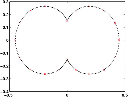
We first consider the linear anisotropic convection-diffusion equation in a square domain $\mathrm{\Omega }=\left\{\left(x,y\right)|0\le x,y\le 1\right\}$

$\frac{{\partial }^{2}u}{\partial x_1^2}+\frac{{\partial }^{2}u}{\partial x_1\partial x_2}+\frac{{\partial }^{2}u}{\partial x_2^2}-\mathbf{v}\cdot \nabla u=0,(20)$

where $k_{11}=k_{22}=1$ and $k_{12}=1/2$ in the constant tensor $\mathbf{K},$ and velocity vector $\mathbf{v}$ is given by $\mathbf{v}={\left[\begin{array}{cc}-\frac{\sqrt{3}}{2}& -\frac{3+\sqrt{3}}{4}\end{array}\right]}^{\text{T}}$.

The analytical solution shown is given as

$u\left(x_1,x_2\right)=\exp \left(-\frac{\sqrt{3}}{2}{x}_1\right)+\exp \left(\frac{1}{2}{x}_1-x_2\right),(21)$

for this case, which is also used to derive the Dirichlet boundary condition.

For the selection of interpolating points, different opinions always exist. Figure 2 shows the average relative error of polynomial $1+r^3$ and MQs whether interpolating points M include boundary collocation points or not. Form Figure 2, we can see the MQs is better than $1+r^3$.

FIGURE 2

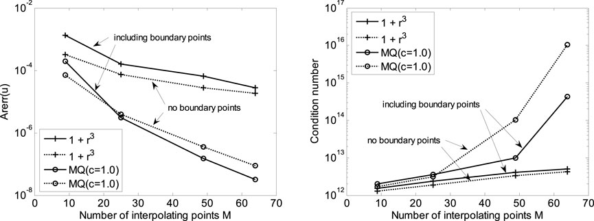
FIGURE 2. Effect of different interpolating schemes with boundary interpolating points and without boundary interpolating points.

For definite internal points number $M=64$, the solution accuracy of the CMFS with different RBFs and its condition numbers with increasing boundary points are shown in Figure 3. It is observed from Figure 3 that accuracy does not show significant improvement when the number of interpolating points maintains. Besides, Figure 4 displays the solution accuracy of the CMFS with different RBFs and its condition numbers with increasing boundary points in solving anisotropic convection-diffusion problems when the number of boundary collocation points $N=36$ is set. We can scrutinize higher convergence rate of the solution accuracy with increasing internal interpolating points than convergence rate with increasing boundary points. Compared to conventional polynomial RBFs, the MQs generally leads to huge condition number of ${10}^{18}$ with corresponding high solution accuracy ${10}^{-7}$. As mentioned in pervious literatures, the better the approximation properties of the RBFs, the worse the conditioning number [43]. In addition, we note that the solution accuracy by using MQs is better than using polynomial RBFs with two or three orders of magnitude. The choice of the RBFs shape parameter is investigated in some literatures [44].

FIGURE 3

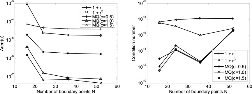
FIGURE 3. Convergence curves of average relative error and condition number with M = 64 by using different interpolating RBFs.

FIGURE 4

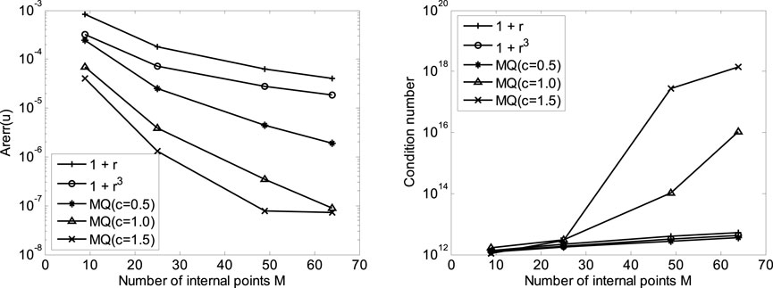
FIGURE 4. Convergence curves of average relative error and condition number with N = 36 by using different interpolating RBFs.

4.2 Nonlinear Inviscid Burger’s Equation

In this case, the nonlinear form for steady-state situation is considered

${\nabla }^{2}u+u\frac{\partial u}{\partial x}=0,(22)$

where the variable $u$ represents a velocity term. A particular solution for this problem is $u\left(x,y\right)=\frac{2}{x}$, which is also the exact solution when imposed as a boundary condition. An peanut irregular domain is considered for this case (Figure 5). The initial guess of $u^{\left(0\right)}$ is selected as one.

FIGURE 5

FIGURE 5. Geometry of a irregular domain for Case 4.2.

Figure 6 shows the convergence curves of the CMFS using the Picard method of iteration with different RBFs. All convergence curves can be found with the increase of internal collocation points $M$. Meanwhile, we also observe that MQ can reach more accuracy when a certain boundary points are employed to implement RBF approximation, instead of pure interior points. However, this phenomenon seems to disappear for $1+r$ and $1+r^3$. Furthermore, the usage of pure internal interpolating points improves accuracy in the case of small M. The similar fact that MQ have better accuracy than polynomials is observed, this is eliminated in this case.

FIGURE 6

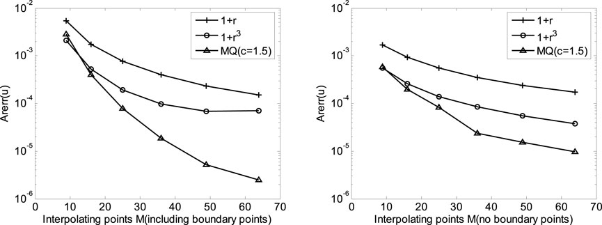
FIGURE 6. Convergence curves of average relative error for nonlinear Burger’s problems with N = 24 by using different interpolation schemes.

4.3 Nonlinear Anisotropic Convection-Diffusion Problem

Consider a 2D anisotropic convection-diffusion problem depicted by

$k_{11}\frac{{\partial }^{2}u}{\partial x^2}+2k_{12}\frac{{\partial }^{2}u}{\partial x\partial y}+k_{22}\frac{{\partial }^{2}u}{\partial y^2}+u\left(\frac{\partial u}{\partial x}+\frac{\partial u}{\partial y}\right)=f(x,y),(23)$

with $k_{11}=k_{22}=1$ and $k_{12}=0.5$ in the same square domain as Example 4.2. The analytical expression $u=0.5\sin \left(x+y\right)$ is used with Dirichlet boundary only, the right-handed source function is chosen to be

$f\left(x,y\right)=-1.5\sin \left(x+y\right)+0.25\sin \left[2\left(x+y\right)\right].(24)$

Here, the similar Picard iteration scheme is employed and the initial guess of $u$ also is set to one. Figure 7 displays the average relative error curve at 1,000 test points against the different interpolating collocation schemes. It is found that whether the boundary collocation is included or not, the CMFS convergence curve converges stably and quickly in solving the nonlinear anisotropic convection-diffusion problem than the polynomial RBFs $1+r$ and $1+r^3$. And the solution accuracy of the CMFS is averagely three orders of magnitude larger than the polynomial RBFS $1+r$ and $1+r^3$. However, the instability for RBF $1+r^3$ should be observed when the RBF approximation involves the usage of the boundary collocation points.

FIGURE 7

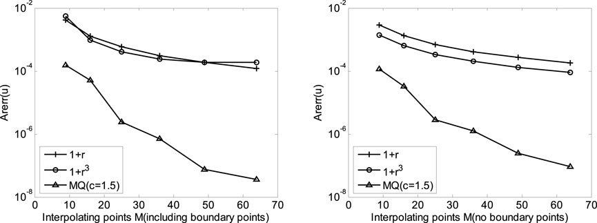
FIGURE 7. Convergence curves of average relative error for anisotropic nonlinear convection-diffusion problems with N = 24 by using different interpolation schemes.

5 Conclusion

In this paper, the CMFS, which is composed by the analog equation method, radial basis function approximation, and the method of fundamental solutions, is applied to the nonlinear anisotropic convection-diffusion problems. Numerical results reveal the efficiency and stability of the CMFS for the tested three cases. In a word, the proposed CMFS has the following features:

1) For linear cases, the approach is just one-step simple scheme. Meanwhile, no inverse of a matrix is involved.

2) The simple fundamental solution of Laplacian operator is employed, rather than one of the original PDE.

3) There are simple process and theoretical basis, so it is easy to program.

4) The related Picard iteration process is developed for nonlinear cases in isotropic and anisotropic media, respectively.

5) The proposed method is a truly meshfree method and no integrals are needed.

6) It can be easily extended to solve anisotropic un-homogeneous problems with variable parameter or the other problems [45].

Data Availability Statement

The original contributions presented in the study are included in the article/Supplementary Material, further inquiries can be directed to the corresponding author.

Author Contributions

LZ supported found of the manuscript; FW developed the conceptualization, and wrote the manuscript; JZ worked on the mathematical development, performed the numerical analysis; SN and TN analyzed the data, and wrote the manuscript. All authors have read and agree to the published version of the manuscript.

Funding

This work is partially supported by the National Natural Science Foundation of China (Project No.U1965110) and the Natural Science Foundation of Anhui Provincial (Project No. 2008085MA11).

Conflict of Interest

The authors declare that the research was conducted in the absence of any commercial or financial relationships that could be construed as a potential conflict of interest.

Publisher’s Note

All claims expressed in this article are solely those of the authors and do not necessarily represent those of their affiliated organizations, or those of the publisher, the editors and the reviewers. Any product that may be evaluated in this article, or claim that may be made by its manufacturer, is not guaranteed or endorsed by the publisher.

References

1. Wang F, Khan MN, Ahmad I, Ahmad H, Abu-Zinadah H, Chu Y-M. Numerical Solution of Traveling Waves in Chemical Kinetics: Time-Fractional Fishers Equations. Fractals (2022) 30(2):2240051. doi:10.1142/S0218348X22400515

CrossRef Full Text | Google Scholar

2. Nadeem S, Fuzhang W, Alharbi FM, Sajid F, Abbas N, El-Shafay AS, et al. Numerical Computations for Buongiorno Nano Fluid Model on the Boundary Layer Flow of Viscoelastic Fluid towards a Nonlinear Stretching Sheet. Alexandria Eng J (2022) 61(2):1769–78. doi:10.1016/j.aej.2021.11.013

CrossRef Full Text | Google Scholar

3. Zhang J, Anjal HA, Msmali A, Wang F, Nofal TA, Selim MM. Heat Transfer of Nanomaterial with Involve of MHD through an Enclosure. Case Stud Therm Eng (2022) 30:101747. doi:10.1016/j.csite.2021.101747

CrossRef Full Text | Google Scholar

4. Wang F, Idrees M, Sohail A. "AI-MCMC" for the Parametric Analysis of the Hormonal Therapy of Cancer. Chaos, Solitons & Fractals (2022) 154:111618. doi:10.1016/j.chaos.2021.111618

CrossRef Full Text | Google Scholar

5. Wang F, Azim Q-U -A, Sohail A, Nutini A, Arif R, R.S. Tavares JM. Computational Model to Explore the Endocrine Response to Trastuzumab Action in HER-2/neu Positive Breast Cancer. Saudi J Biol Sci (2022) 29(1):123–31. doi:10.1016/j.sjbs.2021.08.061

PubMed Abstract | CrossRef Full Text | Google Scholar

6. Zhang J, Wang F, Nadeem S, Sun M. Simulation of Linear and Nonlinear Advection-Diffusion Problems by the Direct Radial Basis Function Collocation Method. Int Commun Heat Mass Transfer (2022) 130:105775. doi:10.1016/j.icheatmasstransfer.2021.105775

CrossRef Full Text | Google Scholar

7. Kansa EJ. Multiquadrics-A Scattered Data Approximation Scheme with Applications to Computational Fluid-Dynamics-I Surface Approximations and Partial Derivative Estimates. Comput Math Appl (1990) 19:127–45. doi:10.1016/0898-1221(90)90270-T

CrossRef Full Text | Google Scholar

8. Zheng H, Yao GM, Kuo LH, Li XX. On the Selection of a Good Shape Parameter of the Localized Method of Approximated Particular Solutions. Aamm (2018) 10:896–911. doi:10.4208/aamm.OA-2017-0167

CrossRef Full Text | Google Scholar

9. Rek Z, Šarler B. The Method of Fundamental Solutions for the Stokes Flow with the Subdomain Technique. Eng Anal Boundary Elem (2021) 128:80–9. doi:10.1016/j.enganabound.2021.03.020

CrossRef Full Text | Google Scholar

10. Hematiyan MR, Mohammadi M, Tsai C-C. The Method of Fundamental Solutions for Anisotropic Thermoelastic Problems. Appl Math Model (2021) 95:200–18. doi:10.1016/j.apm.2021.02.001

CrossRef Full Text | Google Scholar

11. Borachok I, Chapko R, Johansson BT. A Method of Fundamental Solutions for Heat and Wave Propagation from Lateral Cauchy Data. Numer Algor (2022) 89:431–49. doi:10.1007/s11075-021-01120-x

CrossRef Full Text | Google Scholar

12. Gu Y, Fan C-M, Qu W, Wang F, Zhang C. Localized Method of Fundamental Solutions for Three-Dimensional Inhomogeneous Elliptic Problems: Theory and MATLAB Code. Comput Mech (2019) 64:1567–88. doi:10.1007/s00466-019-01735-x

CrossRef Full Text | Google Scholar

13. Xiong J, Wen J, Liu Y-C. Localized Boundary Knot Method for Solving Two-Dimensional Laplace and Bi-harmonic Equations. Mathematics (2020) 8:1218. doi:10.3390/math8081218

CrossRef Full Text | Google Scholar

14. Zhang L-P, Li Z-C, Huang H-T, Chen Z. Super-exponential Growth Rates of Condition Number in the Boundary Knot Method for the Helmholtz Equation. Appl Math Lett (2020) 105:106333. doi:10.1016/j.aml.2020.106333

CrossRef Full Text | Google Scholar

15. Yue X, Wang F, Zhang C, Zhang H. Localized Boundary Knot Method for 3D Inhomogeneous Acoustic Problems with Complicated Geometry. Appl Math Model (2021) 92:410–21. doi:10.1016/j.apm.2020.11.022

CrossRef Full Text | Google Scholar

16. Šarler B. Solution of Potential Flow Problems by the Modified Method of Fundamental Solutions: Formulations with the Single Layer and the Double Layer Fundamental Solutions. Eng Anal Boundary Elem (2009) 33:1374–82. doi:10.1016/j.enganabound.2009.06.008

CrossRef Full Text | Google Scholar

17. Grabski JK. Numerical Solution of Non-newtonian Fluid Flow and Heat Transfer Problems in Ducts with Sharp Corners by the Modified Method of Fundamental Solutions and Radial Basis Function Collocation. Eng Anal Boundary Elem (2019) 109:143–52. doi:10.1016/j.enganabound.2019.09.019

CrossRef Full Text | Google Scholar

18. Zhang L-P, Li Z-C, Huang H-T, Wei Y. The Modified Method of Fundamental Solutions for Exterior Problems of the Helmholtz Equation; Spurious Eigenvalues and Their Removals. Appl Numer Math (2019) 145:236–60. doi:10.1016/j.apnum.2018.09.00810.1016/j.apnum.2019.06.008

CrossRef Full Text | Google Scholar

19. Wang F, Zheng K, Ahmad I, Ahmad H. Gaussian Radial Basis Functions Method for Linear and Nonlinear Convection-Diffusion Models in Physical Phenomena. Open Phys (2021) 19(1):69–76. doi:10.1515/phys-2021-0011

CrossRef Full Text | Google Scholar

20. Schaback R. Limit Problems for Interpolation by Analytic Radial Basis Functions. J Comput Appl Math (2008) 212:127–49. doi:10.1016/j.cam.2006.11.023

CrossRef Full Text | Google Scholar

21. Kazem S, Hatam A. Scattered Data Interpolation: Strictly Positive Definite Radial Basis/cardinal Functions. J Comput Appl Math (2021) 394:113580. doi:10.1016/j.cam.2021.113580

CrossRef Full Text | Google Scholar

22. Shih Y, Elman HC. Iterative Methods for Stabilized Discrete Convection-Diffusion Problems. IMA J Numer Anal (2000) 20:333–58. doi:10.1093/imanum/20.3.333

CrossRef Full Text | Google Scholar

23. Linß T. Anisotropic Meshes and Streamline-Diffusion Stabilization for Convection-Diffusion Problems. Commun Numer Meth Engng (2005) 21:515–25. doi:10.1002/cnm.764

CrossRef Full Text | Google Scholar

24. Onyejekwe OO. Green Element Method for 2D Helmholtz and Convection Diffusion Problems with Variable Velocity Coefficients. Numer Methods Partial Differential Eq (2005) 21:229–41. doi:10.1002/num.20034

CrossRef Full Text | Google Scholar

25. Zhao Y, Wu Y, Chai Z, Shi B. A Block Triple-Relaxation-Time Lattice Boltzmann Model for Nonlinear Anisotropic Convection-Diffusion Equations. Comput Math Appl (2020) 79:2550–73. doi:10.1016/j.camwa.2019.11.018

CrossRef Full Text | Google Scholar

26. Chai Z, Shi B. Multiple-relaxation-time Lattice Boltzmann Method for the Navier-Stokes and Nonlinear Convection-Diffusion Equations: Modeling, Analysis, and Elements. Phys Rev E (2020) 102:023306. doi:10.1103/PhysRevE.102.023306

PubMed Abstract | CrossRef Full Text | Google Scholar

27. Cancès C, Chainais-Hillairet C, Herda M, Krell S. Large Time Behavior of Nonlinear Finite Volume Schemes for Convection-Diffusion Equations. SIAM J Numer Anal (2020) 58:2544–71. doi:10.1137/19M1299311

CrossRef Full Text | Google Scholar

28. Zhelnin MS, Kostina AA, Plekhov OA. Variational Multiscale Finite-Element Methods for a Nonlinear Convection-Diffusion-Reaction Equation. J Appl Mech Tech Phy (2020) 61:1128–39. doi:10.1134/S0021894420070226

CrossRef Full Text | Google Scholar

29. Jha N, Singh B. Fourth‐order Compact Scheme Based on Quasi‐variable Mesh for Three‐dimensional Mildly Nonlinear Stationary Convection-Diffusion Equations. Numer Methods Partial Differential Eq (2020). doi:10.1002/num.22702

CrossRef Full Text | Google Scholar

30. Arrutselvi M, Natarajan E. Virtual Element Method for Nonlinear Convection-Diffusion-Reaction Equation on Polygonal Meshes. Int J Comput Math (2021) 98:1–25. doi:10.1080/00207160.2020.1849637

CrossRef Full Text | Google Scholar

31. Shang J, Chai Z, Wang H, Shi B. Discrete Unified Gas Kinetic Scheme for Nonlinear Convection-Diffusion Equations. Phys Rev E (2020) 101:023306. doi:10.1103/PhysRevE.101.023306

PubMed Abstract | CrossRef Full Text | Google Scholar

32. Cao Z, Zhang LJ, Zhang L. Symmetries and Conservation Laws of a Time Dependent Nonlinear Reaction-Convection-Diffusion Equation. Discrete Cont Dyn-S (2020) 13:2703–17. doi:10.3934/dcdss.2020218

CrossRef Full Text | Google Scholar

33. Katsikadelis JT. The Analog Equation Method: A Boundary-Only Integral Equation Method for Nonlinear Static and Dynamic Problems in General Bodies. Theor Appl Mech (Belgr) (2002) 27:13–38. doi:10.2298/TAM0227013K

CrossRef Full Text | Google Scholar

34. Burlon A, Failla G, Arena F. An Improved Analog Equation Method for Non-linear Dynamic Analysis of Time-Fractional Beams with Discontinuities. Meccanica (2020) 55:649–68. doi:10.1007/s11012-020-01130-4

CrossRef Full Text | Google Scholar

35. Magoulès F, Diago LA, Hagiwara I. Efficient Preconditioning for Image Reconstruction with Radial Basis Functions. Adv Eng Softw (2007) 38:320–7. doi:10.1016/j.advengsoft.2006.08.012

CrossRef Full Text | Google Scholar

36. Fairweather G, Karageorghis A. The Method of Fundamental Solutions for Elliptic Boundary Value Problems. Adv Comput Math (1998) 9:69–95. doi:10.1023/A:1018981221740

CrossRef Full Text | Google Scholar

37. Liu C-S. The Method of Fundamental Solutions for Solving the Backward Heat Conduction Problem with Conditioning by a New Post-conditioner. Numer Heat Transfer, B: Fundamentals (2011) 60:57–72. doi:10.1080/10407790.2011.588134

CrossRef Full Text | Google Scholar

38. Gorzelańczyk P, Kołodziej JA. Some Remarks Concerning the Shape of the Source Contour with Application of the Method of Fundamental Solutions to Elastic Torsion of Prismatic Rods. Eng Anal Boundary Elem (2008) 32:64–75. doi:10.1016/j.enganabound.2007.05.004

CrossRef Full Text | Google Scholar

39. Fasshauer GE, Zhang JG. On Choosing “Optimal” Shape Parameters for RBF Approximation. Numer Algor (2007) 45:345–68. doi:10.1007/s11075-007-9072-8

CrossRef Full Text | Google Scholar

40. Schaback R. Adaptive Numerical Solution of MFS Systems. In: CS Chen, A Karageorghis, and YS Smyrlis, editors. The Method of Fundamental Solutions-A Meshless Method. Atlanta: Dynamic Publishers (2008). p. 1–27.

Google Scholar

41. Reddy GMM, Nanda P, Vynnycky M, Cuminato JA. An Adaptive Boundary Algorithm for the Reconstruction of Boundary and Initial Data Using the Method of Fundamental Solutions for the Inverse Cauchy-Stefan Problem. Comp Appl Math (2021) 40:99. doi:10.1007/s40314-021-01454-1

CrossRef Full Text | Google Scholar

42. Bavestrello H, Avery P, Farhat C. Incorporation of Linear Multipoint Constraints in Domain-Decomposition-Based Iterative Solvers - Part II: Blending FETI-DP and Mortar Methods and Assembling Floating Substructures. Comput Methods Appl Mech Eng (2007) 196:1347–68. doi:10.1016/j.cma.2006.03.024

CrossRef Full Text | Google Scholar

43. Liu C-S, Chang C-W. A Simple Algorithm for Solving Cauchy Problem of Nonlinear Heat Equation without Initial Value. Int J Heat Mass Transfer (2015) 80:562–9. doi:10.1016/j.ijheatmasstransfer.2014.09.053

CrossRef Full Text | Google Scholar

44. Wang F, Hou E, Ahmad I, Ahmad H, Gu Y. An Efficient Meshless Method for Hyperbolic Telegraph Equations in (1 + 1) Dimensions. Cmes-comput Model Eng (2021) 128(2):687–98. doi:10.32604/cmes.2021.014739

CrossRef Full Text | Google Scholar

45. Wang F, Varun Kumar RS, Sowmya G, El-Zahar ER, Prasannakumara BC, Khan MI, et al. LSM and DTM-Pade Approximation for the Combined Impacts of Convective and Radiative Heat Transfer on an Inclined Porous Longitudinal Fin. Case Stud Therm Eng (2022) 101846. doi:10.1016/j.csite.2022.101846

CrossRef Full Text | Google Scholar