Cascaded Progressive Generative Adversarial Networks for Reconstructing Three-Dimensional Grayscale Core Images From a Single Two-Dimensional Image

It is very challenging to accurately understand and characterize the internal structure of three-dimensional (3D) rock masses using geological monitoring and conventional laboratory measures. One important method for obtaining 3D core images involves reconstructing their 3D structure from two-dimensional (2D) core images. However, traditional 2D–3D reconstruction methods are mostly designed for binary core images, rather than grayscale images. Furthermore, the reconstruction structure cannot reflect the gray level distribution of the core. Here, by combining the dimension promotion theory in super-dimension (SD) reconstruction and framework of deep learning, we propose a novel convolutional neural network framework, the cascaded progressive generative adversarial network (CPGAN), to reconstruct 3D grayscale core images. Within this network, we propose a loss function based on the gray level distribution and pattern distribution to maintain the texture information of the reconstructed structure. Simultaneously, by adopting SD dimension promotion theory, we set the input and output of every single node of the CPGAN network to be deep gray-padding structures of equivalent size. Through the cascade of every single node network, we thus ensured continuity and variability between the reconstruction layers. In addition, we used 3D convolution to determine the spatial characteristics of the core. The reconstructed 3D results showed that the gray level information in the 2D image were accurately reflected in the 3D space. This proposed method can help us to understand and analyze various parameter characteristics in cores.

1 Introduction

Current on-site geological monitoring approaches struggle to accurately understand and characterize the three-dimensional (3D) structural properties of rock mass [1].

The most commonly used method to solve this problem entails obtaining detailed information on the rock structure using physical imaging equipment [2–7]. Taking computed tomography (CT) as an example, the gray values of pixels in a 3D-core CT image comprehensively reflect the differences in the X-ray absorption coefficients of different rock components [8]. Real rock samples are usually composed of multiple components, and these different components show different gray values under imaging equipment. Specifically, the core parameter characteristics, such as permeability [9–11], electrical conductivity [12–14], and elastic modulus [15–17], will also vary with the distribution of these components. 3D gray core CT images are of great significance for studying core compositions and their physical characteristics [18–26].

Digital core reconstruction methods can be divided into two categories. The first is direct imaging, which uses various optical or electronic equipment (such as CT) to scan and image the rock sample and perform 3D reconstruction. This reconstruction method requires interpolation. The second is to extract feature information from a two-dimensional (2D) image and use mathematical methods for 3D reconstruction. This method involves reconstruction from a single 2D image to a 3D structure with the addition of certain prior information in the absence of interpolation.

However, for direct imaging, owing to high costs, computational difficulties, and the long length of time required, obtaining 3D data sets through physical imaging equipment for different samples has its limitations. Notably, high-resolution 2D images can be obtained easily at a low cost [27]. 2D–3D reconstruction does not require the reconstruction results to reproduce the same structure exactly; it only requires that the reconstruction results and the target system are similar in terms of statistical and morphological features. Based on the above mentioned reasons, it would be extremely valuable to be able to reconstruct the 3D structure of a sample based on a single 2D image [28–32]. Most of the current research in this regard is based on binary images; however, research into the reconstruction of gray core images is still relatively rare.

Compared with the reconstruction of binary cores, gray cores are more difficult to reconstruct because there are 256 gray levels, which makes it more difficult to describe their complex statistical and morphological characteristics. Learning these features and building a map for their reconstruction are the key actions required to solve this problem. Deep learning and super-dimension (SD) reconstruction theory [33–36], which has been widely used in binary core reconstruction, is a better strategy for establishing a map than traditional methods.

SD theory borrows the concepts of “mapping relationship,” “prior model,” and “training dictionary,” from learning-based super-resolution reconstruction [37–40] and applies them to the 3D reconstruction of porous media. In the training stage, the mapping relationship between the 2D patches and the 3D blocks in the real core is learned; this is used as prior information to guide the subsequent reconstruction of a single 2D image.

Machine learning (ML)-based methods [41–44] have become increasingly popular because they can predict end-to-end (2D–2D and 2D–3D) material properties to accelerate the design of new materials. Recent advances in “deep learning” have made it possible to learn from raw data representations [45, 46], such as the pixels of an image. This makes it possible to build a universal model that is superior to traditional expert-designed representations. At present, deep learning methods are mostly used to reconstruct binary cores [47].

In this study, we designed the cascaded progressive generative adversarial network (CPGAN) by combining the deep learning method [48–50] and idea of dimension promotion in the SD concept. Based on this network, we proposed a gray-core image reconstruction algorithm. The inspiration for this design comes from the following sources: in the field of deep learning, the newly emerged bicycleGAN [51] can achieve image-to-image style conversion. Therefore, to solve the problem of mode number explosion for the dictionary patterns of gray core images, here we attempted to establish a mapping function relationship through deep learning, to maintain the texture information of the reconstructed structure. Simultaneously, by borrowing the idea of gradual reconstruction in SD dimension promotion, we designed a cascading peer information network to achieve continuity and variability between reconstruction layers.

The remainder of this paper is organized as follows. The backgrounds of GAN and SD reconstruction are introduced in Section 2. The proposed CPGAN network and its related 3D grayscale core image reconstruction algorithms are described in Section 3. Section 4 describes and analyzes the results of the experiments performed, and a summary of this study is presented in Section 5.

2 Background of Generative Adversarial Network and Super-Dimension Reconstruction

2.1 Generative Adversarial Network and Mapping in the Reconstruction of 3D Digital Cores

The GAN is composed of two opposing models: the generator and the discriminator. The generator attempts to learn the distribution characteristics of a given dataset to generate near-real data to trick the discriminator. The discriminator then judges the authenticity of the generated results given by the generator by estimating the probability. The network structure parameters are continuously optimized through a continuous game between these two models. Finally, the generator produces the required result, which is almost indistinguishable from the real data, which is given by

$\underset{G}{\min }\underset{D}{\max }V(D,G)=E_{x\sim p_{data}\left(x\right)}[\log D\left(x\right)]+E_{z\sim p_z\left(z\right)}\left[\log (1-D\left(G\left(z\right)\right))\right](1)$

where G is the generative model, D the discriminative model, z the noise, Pz(z) the prior noise distribution, x the input data, and V(D, G) the value function.

By adding additional constraints, y, to the discriminator and generator, we can obtain a conditional GAN (CGAN) whose expression is as follows:

$\underset{\text{G}}{min}\underset{D}{max}V(D,G)=E_{x\sim p_{data}\left(x\right)}\left[logD\left(x\right|y)\right]+E_{z\sim p_z\left(z\right)}\left[log(1-D\left(G\left(z\right|y)\right))\right](2)$

GAN-based deep learning methods have been gradually recognized in the field of digital cores and demonstrated to have a very good performance. Regarding the reconstruction of core images, current research is still focused on binary image reconstruction. The schematic diagram of synthesis and reconstruction of binary images is attached as Supplementary Material S1. These applications have great potential for the reconstruction of 3D structures from 2D gray core images.

2.2 Gradual Reconstruction in the Super-Dimension Promotion Process

The complete process of the SD reconstruction framework can be divided into the dictionary building stage and reconstruction stage. In the dictionary building stage, a set of real cores is selected. Then, a 2D template of size N × N and a 3D mapping template of size N × N × N are selected. Afterward, the mapping template is used to access the real core along the raster path to obtain dictionary elements. Next, a mapping relationship between the acquired 2D image mode and the corresponding 3D image mode is established, and they are stored as dictionary elements to form a dictionary. In the process of scanning the real core with the mapping template, the acquired 2D image pattern will have a large number of repetitions, and the same 2D image will correspond to multiple 3D blocks. The atomized 2D–3D matching pair in the real core is obtained and used as prior information. Based on this, different learning mechanisms are used to learn the mapping relationships in the real core to guide the reconstruction. In the reconstruction stage, the current 2D reference image to be reconstructed is traversed along the raster path with the size of N × N template, and the obtained 2D block is used to search for the best matching 3D block in the dictionary through the learned SD mapping relationship. After the entire reference image is searched and matched, the current N-layer images is reconstructed, and then, the uppermost 2D image is used as a new training image to repeat the aforementioned reconstruction process, until the entire 3D structure has been reconstructed. The schematic diagrams of the dictionary building stage and reconstruction stage of SD algorithm are attached as Supplementary Material S1. The SD reconstruction process adopts a systematic progressive reconstruction. The previous reconstruction information can be used as a constraint condition for the next step, thereby maintaining the continuity and variability between layers.

$X_{MAP}=\arg \min \left[{\displaystyle \sum _{k=1}^p{\Vert B_{k}X-y_k\Vert }^2+\lambda \gamma \left(X\right)}\right](3)$

The 3D reconstruction of the digital core can be expressed using the mathematical model shown in Eq. 3. This formula represents the process of estimating the corresponding 3D spatial structure X based on a single 2D reference image y_k, with the addition of regularization terms γ(x) as prior knowledge. Here, B_k is the dimensionality reduction matrix, X the reconstruction result obtained through maximum posterior probability estimation, and λ the regularization coefficient.

2.3 Advantages and Disadvantages of Using Generative Adversarial Network and Super-Dimension Methods in Grayscale Core Reconstruction

The key to using GAN to reconstruct a 3D grayscale core image from a single 2D image lies in determining how to build a 2D-to-3D map under the condition of information equivalence. GANs are commonly used to reconstruct binary images. If a single 2D gray image was taken as the input and the entire 3D gray core image as the target of the GAN network, this inequality created between the input and output information would increase the solution space of the generated structure, which is not conducive to the training of the entire network. Under this condition, the reconstructed grayscale core structure could maintain grayscale texture information but would not be able to maintain continuity and variability between layers.

When using the SD reconstruction method to reconstruct grayscale core images, compared with the reconstruction of binary core images, the mapping relationship between the 2D patches and the 3D blocks of the gray core images becomes more complicated. If the SD method is used in the reconstruction of grayscale core images, a dictionary containing the mapping relationship between the 2D gray level patches and the 3D gray level blocks should be established. Consider as an example a template of size N × N. For a binary core, the number of pixel modes in the dictionary is 2N × N. However, for a grayscale image, the number of modes increases sharply to 256N × N. The direct consequence of this is the incompleteness of the SD dictionary. In the later stages of reconstruction, textures and pattern information would gradually disappear owing to matching errors. However, owing to progressive reconstruction, the continuity and variability between layers would be maintained during reconstruction.

3 Materials and Methods

3.1 Materials

The cores used for conventional research are typically cylinders with a diameter of 25–100 mm. If a clear image of the micron or nanoscale pore structure is to be obtained, the core can be cut into a few millimeters or smaller. In this study, to obtain a training image, the columnar cores were first obtained, with a diameter of 25 mm and image pixel length of 13.6 μm. These cores were then cut and scanned by CT. The final core diameter and image pixel length were 2 mm and 1 μm, respectively. Slice thickness refers to the (often, axial) resolution of the scan. Here, the resolution of the final obtained CT slice was 1 μm.

The resolution of the CT image to be reconstructed is related to the quality of the reconstructed structure. The higher the resolution, the more detailed the information obtained. In this study, the resolution of the reconstructed 3D structure by the proposed method depends on the resolution of the 2D image to be reconstructed (1 μm in this study).

Different materials have different differential opacities. The gray value of the pixel in the 3D core CT image comprehensively reflects the difference in the X-ray absorption coefficient of different components of the rock. In this study, the deep learning network CPGAN can establish a mapping from a 2D plane to a 3D space for reconstructing different materials with differential opacities.

3.2 Methods

In our previous research on binary core reconstruction, the original SD algorithm was proposed by establishing 2D and 3D matching pairs as the dictionary [34]. In this study, for the reconstruction of grayscale core images, the mapping relationship is more complicated. In establishing a 2D-to-3D mapping relationship of grayscale cores, the major research problem is how to maintain both textural and inter-layer information during the reconstruction process to ensure the reconstructed structure is consistent with the real situation.

To address this problem, both deep learning and SD methods have distinct advantages. The mapping function relationship established by the deep learning method can maintain the textural information of the reconstructed structure, but the continuity and variability between the layers of the 3D structure cannot be maintained. By contrast, dimension promotion in SD can realize continuity and variability between layers of reconstruction. How to combine these two ideas organically is essential in solving the problem.

This study is novel in its attempt to establish a mapping function through deep learning for maintaining the textural information of the reconstructed structure. Simultaneously, the idea of progressive reconstruction in SD theory is utilized, and cascade every single network whose input and output are peer-to-peer structures. This is necessary to achieve continuity and variability between the reconstruction layers. Based on the aforementioned information, this research proposes CPGAN to reconstruct gray core images. The details of this method are analyzed further.

To establish 2D to 3D mapping under the condition of equal information and to use 3D convolution to learn 3D spatial information, we designed the CPGAN and set the input and target of each single-layer node network in the CPGAN cascade network to be two 3D volumes with a peer structure (as explained in paragraph 4 of Section 3.2.2). The specific design of the network is as follows.

3.2.1 Deep Gray Padding

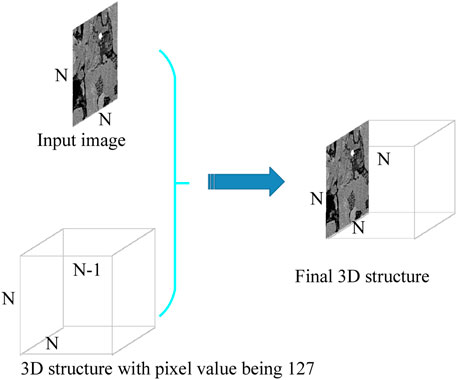
In this study, we used a deep gray-padding technology to fill the input and output 2D images into a 3D structure, with a size similar to that of the final reconstructed target. This ensured that the network learned the mapping relationship between the 3D input and the 3D output. Figure 1 show a schematic diagram of the deep gray padding. This type of network learning is simpler than learning the relationship from 2D to 3D images. Similar techniques have also been used for pedestrian re-identification [52]. Suppose the dimensions of the input image are 1 × N × N, that it is filled with a 3D volume with size (N-1) × N × N, and that all pixel values are 127. The size of the final 3D structure would be N × N × N.

FIGURE 1

FIGURE 1. Schematic diagram of deep gray padding.

3.2.2 Cascade Network Architecture

The CPGAN architecture is composed of node networks in the training stage and a cascaded network in the reconstruction stage.

In the training stage, for a grayscale core reference image of size n², log₂n node networks are required: the trained generators are cascaded in the reconstruction stage. Here, we used a 128 × 128 image as a reference image for reconstruction. In this case, seven-node networks were required during the training stage. For the k^th-node network (1 ≤ k ≤ 7), the input images were 2^k−1 continuous images in the CT sequence, which were padded using the method described in Section 3.2.1. The output images are 2^k continuous CT slices including the 2^k−1 input, which will also be padded.

Under these conditions, we were able to progressively train a mapping relationship with input and output structures that had overlapping parts; this is similar to the idea of dimension promotion in SD theory. Thus, the continuity and variability between the layers were maintained. Besides, as deep learning technology was used to establish the map, the grayscale texture information was maintained. Figures 2A,B show the first and third node networks in the training stage, respectively.

FIGURE 2

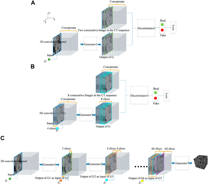
FIGURE 2. Schematic diagram for the training and reconstruction stage of CPGAN. (A) The first node networks in the training process of CPGAN; (B). The third node networks in the training process of CPGAN; (C) The reconstruction stage of CPGAN.

The inputs and outputs of CPGAN’s node network comprised a peer-to-peer structure because they are all 3D objects of the same size. The advantages of adopting this peer-to-peer structure are twofold. On the one hand, we can use the 3D convolution kernel to learn the 3D spatial information of the grayscale core image. On the other hand, 2D to 3D grayscale core image reconstruction, which is an ill-conditioned problem with unbalanced input and output information, is converted to a problem of gradual reconstruction. The first node network can be regarded as mapping from a 2D image to a 2D image and the node network after as mapping from a 3D image to a 3D image. This reduces the information difference between the input and output in the entire process.

For every node network, the generator’s network structure is still based on the classic U-Net. Notably, to better capture 3D spatial information, we used both 3D convolution and 3D transposed convolution. However, the 3D convolution operation greatly complicates the process of training the network, resulting in an insufficient graphics processing unit (GPU) memory. To solve this problem, we cancelled the final channel fusion process, as 3D (transposed) convolution itself is an operation performed in 3D, which can effectively fuse information between channels. In traditional GAN, after the image enters the generator, it is downsampled stepwise to a size of 1 × 1. Regarding the algorithm proposed in this paper, previous experiments have shown that image downsampling to a size of 2 × 2 has little influence on the final accuracy but that this strategy can reduce the network parameters by approximately 30%, save GPU memory, and accelerate network convergence. For the abovementioned reasons, we downsampled the image to a size of 2 × 2.

A schematic diagram of the reconstruction stage of the CPGAN is shown in Figure 2C. Here, the n generators that were trained as described earlier were cascaded (when the reference image size is 128, n = 7). The input is a 3D volume with a reference image as the first layer and other layers were padded with pixels with a gray value of 127. This 3D body was first sent to the first layer of CPGAN, and its output was used as the input for the next layer of the network. We repeated the abovementioned operations to reconstruct 2n images from the original reference image. By stacking these 2n images, the entire 3D structure can be reconstructed. The cascade formula for CPGAN is

$Output=G_7\left(G_2\left(G_1(input,z),z\right),z\cdots ,z\right)(4)$

3.2.3 Histogram matching Constraints for Cascaded Progressive Generative Adversarial Network

The traditional BicycleGAN network uses the weighting of the CGAN loss function, L_GAN, and uses the L1 loss function, L_L1, as the final loss function. The purpose of CPGAN as proposed here is to reconstruct the gray core images. Therefore, it is necessary to propose a new loss function specifically for reconstructing gray core images. It is also necessary to achieve a better reconstruction effect by weighting and summing with the previous L_GAN and L_L1 loss values.

3.2.3.1 L_{grayscale Pixel value}—Histogram matching Constraints Based on the Grayscale Pixel Value Distribution

Traditionally, the loss function is used to measure the difference between the predicted value of the network and the true value. The calculated loss is back propagated to update the parameters. The loss function of the common GAN generator is defined as follows:

$L_{CGAN}\left(G\right)=x\sim p(x)[D{(x,G(x)-1]}^2(5)$

where x is the input, G the generator, D the discriminator, and E the expectation. Eq. 5 shows that the goal of G is to expect the generated fake sample to be judged as 1 (true) by the discriminator. That is, it hopes to produce a more realistic image and achieve the purpose of deceiving the discriminator.

For the reconstruction problem in this study, Eq. 5 only indicates that the fake sample, G(x), is (visually) similar to the real sample. Furthermore, it does not restrict the grayscale distribution of the pores and rock. To reflect this constraint, we added loss to measure the point-to-point difference of the grayscale pixel value between the reconstruction result and the target image. The specific definition is as follows:

$L_{grayscalepixelvalue}={\displaystyle \sum _0^{255}{\Vert {\mathrm{B}}_{grayscalepixelvalue}-{\widehat{\mathrm{B}}}_{grayscalepixelvalue}\Vert }_2^2}(6)$

Here, B_{grayscale pixel value} represents the pixel value distribution of the real image, and ${\widehat{B}}_{grayscalepixelvalue}$ represents the pixel value distribution of the reconstruction result.

3.2.3.2 L_{grayscale pattern}—Histogram matching Constraints Based on the Grayscale Pattern Distribution

Similar to the pattern set in multipoint geostatistics, the grayscale pattern distribution in the grayscale core image can reflect its morphological characteristics. The advantage of using a smaller pattern is that the GPU memory requirement is small and the matching speed is fast. The disadvantage is that the long-range information of the obtained image is limited. The advantage of using a larger pattern is that more information in the long-range can be obtained, but the disadvantage is that the GPU memory requirement is large and the matching speed is slow. Therefore, in CPGAN, we propose a loss function based on the grayscale pattern distribution to measure the difference between the predicted value, G(x, z), and the true value in the pattern distribution, B. The specific definition is as follows:

$L_{grayscalepattern}={\Vert {\mathrm{B}}_{grayscalepattern}-{\widehat{\mathrm{B}}}_{grayscalepattern}\Vert }_2^2(7)$

In this formula, B_{grayscale pattern} represents the grayscale pattern distribution of the real image, and ${\widehat{B}}_{grayscalepattern}$ represents the grayscale pattern distribution of the reconstruction result. Here, a grayscale pattern in the image is defined as data composed of multiple points captured by an N × N template. Taking a 3 × 3 template as an example, Figure 3 shows the calculation process of the pattern distribution. Specifically, this process comprised the following steps: 1) scan the slices in x, y, z directions of the 3D target and the generator output of G((x,z)) with a template to collect all patterns that appear, Pat_i; 2) flatten each pattern and perform binarization to obtain its corresponding binary code and then convert it into a decimal number, PatNum_i; and 3) count the occurrences of each Pat_i to get Num(Pat_i) and then normalize it to get the probability, P_i, of each pattern. P_i is defined as shown in Eq. 8, in which N_total represents the sum of the numbers of all patterns in an image:

$p_i=\frac{NUM\left(Pa{t}_i\right)}{N_{total}}(8)$

FIGURE 3

FIGURE 3. Schematic diagram for the reconstruction stage of CPGAN.

3.2.3.3 L_{total loss}—Total Loss Function

In CPGAN, the total loss function is the weight of L_GAN, L_L1, L_{grayscale pixel value}, and L_{grayscale pattern}. It can be expressed as shown in Eq. 9. Here, the λ_{grayscale pixel value} and λ_{grayscale pattern} represent the weights of the grayscale pixel value loss and the grayscale pattern loss, respectively. The basic principle of the loss function weight setting is to ensure that the contribution of each part of the loss to the total loss is similar. If the weight is set too small, the loss will not constrain the network enough; if the weight is set too large, the loss will contribute too much to the total loss, and the network will have difficulty learning the constraints of other loss functions. In this research, the λ_{grayscale pixel value} and λ_{grayscale pattern} were set to be 1,000 and 5 × 10⁵, respectively.

$L_{totalloss}=L_{CGAN}+L_{L1}+{\lambda }_{pattern}{L}_{pattern}+{\lambda }_{grayscalepixelvalue}{L}_{grayscalepixelvalue}(9)$

4 Experimental Results and Discussion

4.1 Relationship Between the Structure Size, Network, and Reconstruction Time

The running environment of the experiment in this section was as follows: the CPU model was Intel i7-6700k, RAM was 16 GB DDR3, GPU model was Nvidia GTX 1080, and the operating system was Ubuntu 16.04. It took 0.5 s to reconstruct a core image with a size of 128³ pixels. The reconstruction time is proportional to the amount of network input data, for a core image of size n³ in terms of the amount of data, n³ = 128³ × (n/128)³. Thus, the reconstruction time is approximately (n/128)³ times the reconstruction time of the 128³ size core image; that is, (n/128) 3× 0.5 s.

4.2 Experimental Basis and Network Parameter Settings

Batch size is an important parameter in network design based on deep learning. It is related to the GPU memory cost and training speed. Every time we send a part of the data in the training set to the network, and this part of the data is called a batch. The amount of this part of the data is called the batch size. It indicates the number of data passed to the program for training at a time. For example, our training set has 1,000 pieces of data. In this case, if we set the batch size to 100, then the program will first train the model with the first 1–100th data. The batch size cannot be too large or too small. If the batch size is too small, the gradient of the entire network will constantly change, and thus the network will not converge. If the batch size is too large, this will cause insufficient memory, slow parameter modification, and slow network convergence. Based on these factors and after continuous experiments, we set the batch size to four (4 sets of data in the training set) to achieve an optimal network performance.

The learning rate is the step size of the gradient descent. A very small learning rate will ensure that the gradient approaches the minimum value during training. Thus, the minimum value will not be missed, but the corresponding training speed will be slow. If the learning rate is high, the training may cross the minimum value and fluctuate frequently. Based on these considerations, we set the learning rate to 0.0002.

In terms of software configuration, we used an Nvidia GTX 1080 GPU and the Pytorch deep learning framework to build CPGAN for the reconstruction of 3D gray core images.

4.3 Visual Effects of Reconstruction Results

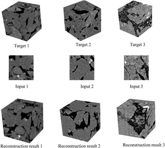
To prove the universality of CPGAN, we selected three sets of gray core sample images composed of different rock components for the experiments. A schematic of the CPGAN reconstruction results is shown in Figure 4. In Figure 4, inputs 1, 2, and 3 are slices randomly selected from targets 1, 2, and 3, respectively. Visually comparing the target system and the reconstructed structure revealed that they have similar morphological characteristics, indicating that our proposed algorithm can successfully reconstruct gray core images. Furthermore, the components in the 2D image were well reflected in the 3D structures, indicating that CPGAN successfully learned the relationship between the component information in the 2D image and the 3D space.

FIGURE 4

FIGURE 4. Schematic diagram of CPGAN reconstruction results.

4.4 Comparative Experiments

In this section, we compare the results of the gray cores reconstructed by the SD and CPGAN algorithms. SD is an algorithm used for binary-image reconstruction. For comparison, the dictionary of the SD algorithm is obtained from grayscale core CT sequence images, which are then used for grayscale core image reconstruction. During reconstruction, a 5 × 5 size 2D template is used to traverse the training images to build a dictionary. For the purposes of this comparison, we trained CPGAN according to the method described in Section 3 to establish the related mapping relationship.

The gray core reference image and the target system that we used in this experiment are shown in Figures 5A,B, respectively. The structures reconstructed using the SD and CPGAN algorithms and their cross-sectional views are shown in Figures 5C–F. A visual comparison of the reconstruction effects revealed that the target system and the reconstructed structure of the CPGAN exhibited more similar morphological characteristics than the other structure. This indicates that the algorithm described in this paper was best at reconstructing the gray core image.

FIGURE 5

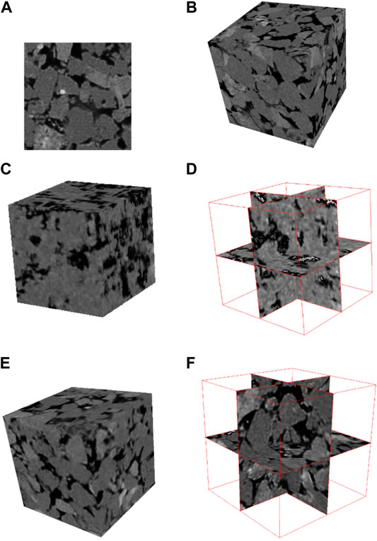
FIGURE 5. Comparison of gray core images reconstructed by SD and CPGAN. (A) Reference image; (B) target sample; (C) SD algorithm reconstruction structure; (D) cross-section of the structure reconstructed by SD; (E) CPGAN algorithm reconstruction structure. (F) cross-section of structure reconstructed by CPGAN.

Based on the experiment shown in Figure 5, we compared sliced images of the reconstruction results of the two algorithms. The sliced images of the reconstruction structures of the SD algorithm are shown in Figures 6A–D. The sliced images of the reconstruction structures of the CPGAN algorithm are shown in Figures 6E–H, respectively.

FIGURE 6

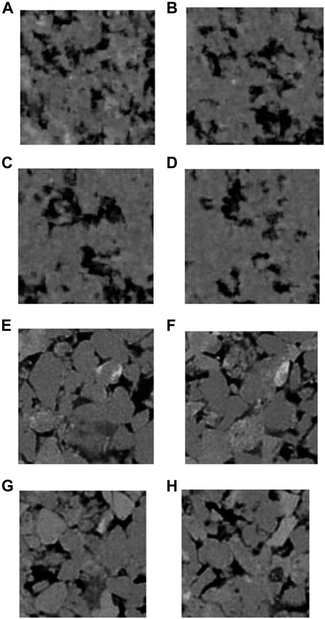
FIGURE 6. Cross-sectional view of structure reconstructed by the SD algorithm (A–D) and the CPGAN algorithm (E–H).

Regarding the grayscale core images reconstructed by the SD algorithm, although there were continuity and variability between the layers of the reconstruction structure, the large number of modes meant that the dictionary was relatively incomplete; this likely resulted in the gradual disappearance of mode information in the later stage of reconstruction, such as the grayscale texture. The CPGAN algorithm not only achieved continuity and variability between the layers of the reconstructed structure but also maintained the textural information through a combination of GAN and SD theory. In the remainder of this section, we used different parameters to quantitatively analyze the reconstruction results.

4.4.1 Variogram

Variogram is a statistic that describes the spatial correlation of a random field or a random process, and is defined as the variance between two points in space. The formula for Variogram is derived as follows: let the regionalized variable Z(x) satisfy the (quasi) eigen hypothesis, h is the spatial separation distance between the two sample points, and Z(x_i) and Z(x_i + h) are respectively the observed value of Z(x) at the spatial positions x_i and x_i+h (i = 1, 2,...N(h)), then the formula for calculating the experimental variogram is:

$\gamma \left(h\right)=\frac{1}{2N\left(h\right)}{\displaystyle \sum _{i=1}^{N\left(h\right)}{[Z\left(x_i\right)-Z(x_i+h)]}^2}(10)$

Here, N(h) represents the number of sample pairs when the separation distance is h.

To further quantify the reconstruction results of the grayscale core image, we compared the variogram of the target sample with the reconstruction structures of the SD and CPGAN algorithms. The comparison curve is shown in Figure 7A. Through the analysis of Figure 7A, it can be seen that the CPGAN reconstruction structure better reproduced the 3D spatial correlation of the target sample. Due to the loss of grayscale information in the reconstruction process by SD algorithm, the variogram of SD is slightly lower than the other two curves as a whole.

FIGURE 7

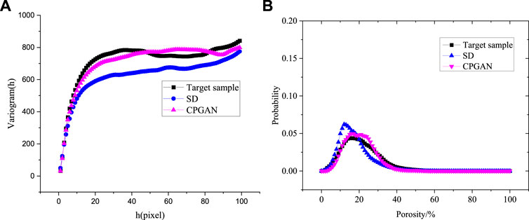
FIGURE 7. Comparison curve of the variogram (A) and local porosity (B) between target sample and reconstructed structure for different algorithms.

4.4.2 Local Pore Distribution Function

In this section, we used the local porosity distribution function [53, 54] to further compare the morphological similarities between the reconstruction result and the target system as shown in Figure 5. This characteristic function is a higher-order statistical function that can effectively describe the spatial distribution of 3D pores. It is defined as follows:

Let us suppose there is a sample of porous media, S∈R³. If the sample includes only the grain phase, M, and the pore phase, P, then $S=P\cup M$ and $P\cap M =Ø$. $K\left(\stackrel{\rightharpoonup }{\text{c}},L\right)$ is a measuring unit in porous media, which is a subset of S and represents a cube with points $\stackrel{\rightharpoonup }{c}$ as the center and L as the side lengths inside the porous media. Then, the local porosity, $\varphi \left(\stackrel{\rightharpoonup }{\text{c}},L\right)$, can be expressed as

$\varphi \left(\stackrel{\rightharpoonup }{c},L\right)=\frac{V\left(P\cap K\left(\stackrel{\rightharpoonup }{c},L\right)\right)}{V\left(K\left(\stackrel{\rightharpoonup }{c},L\right)\right)}(11)$

Here, V(T) represents the volume of the phases T and T∈R³. Based on the definition of local porosity, the local pore distribution function is defined as

$\mu \left(\varphi ,L\right)=\frac{1}{m}{\displaystyle {\sum }_{\stackrel{\rightharpoonup }{r}}\delta \left(\varphi -\varphi \left(\stackrel{\rightharpoonup }{c},L\right)\right)}(12)$

Here, $\text{δ}\left(x\right)$ is the Dirac function and m represents the number of measurement units. The physical meaning of the local pore distribution function is as follows: given any measurement unit, $K\left(\stackrel{\rightharpoonup }{c},L\right)$, the probability of its porosity within the range $\varphi \to \varphi +\text{d}\varphi$ is  $\mu \left(\varphi ,L\right)$ $\varphi$ is the volume porosity.

The distribution curve of the local porosity distribution function, $\mu \left(\varphi ,L\right)$ can be used to determine the structural characteristics of the degree of homogeneity of the porous medium. When the size of the measurement unit, L, is fixed with porosity, $\varphi$, as an independent variable, the function $\mu \left(\varphi ,L\right)$ reflects the distribution of porosity across the entire porous medium. The distribution concentration reflects the degree of structural homogeneity. The more concentrated the curve distribution, the better the homogeneity.

We also compared the abovementioned characteristics of the target system and the reconstructed results from SD, and CPGAN (Figure 5). Figure 7B shows the comparison results. The distribution and peak breadths of the local porosity of the target were similar to those of the structure reconstructed by CPGAN. This indicates that the 3D pore space distribution and degree of homogeneity of the structure reconstructed by CPGAN were more similar to those of the target than to those of SD.

4.4.3 Gray Level Co-Occurrence Matrix

The statistical method of GLCM was proposed by Haralick et al. in the early 1970s. This is a classic and vital texture feature extraction method. It has been widely used in image classification, image segmentation, and other fields because of its simple and effective calculation. Essentially, the GLCM describes the joint conditional probability distribution of two pixels in space as: $\text{G}(i,j|d,\theta )$. It reflects the comprehensive information of the image in the direction, interval, range, and speed of change by calculating the correlation between the grayscale of two points in the image at a certain distance and in a certain direction. In this probability distribution, i and j represent the gray values of these two pixels, respectively, and d and $\theta$ represent the distance and angle relationship between them, respectively. A typical schematic diagram for GLCM calculation is attached as Supplementary Material S1, in which d = 1 and $\theta =\text{0}$.

Generally, some scalars can be used to characterize the features of a GLCM. Some common features of the GLCM are as follows:

Energy (angular second moment; ASM): energy is the sum of the squares of the element values of the GLCM; it reflects the uniformity of the image grayscale distribution and the thickness of the texture. Its expression is

$\text{ASM}={{\displaystyle {\sum }_{i=1}^k{\displaystyle {\sum }_{j=1}^k\left(G(i,j)\right)}}}^2(13)$

Entropy (ENT): entropy is used to measure the degree of disorder of the pore distribution in an image. The larger the value, the more scattered the element values are in the matrix. If there is no texture in the image, then this value will be smaller, whereas if the image’s texture is complex, the value will be larger. Its expression is as follows:

$ENT=-{\displaystyle {\sum }_{i=1}^k{\displaystyle {\sum }_{j=1}^{k}G(i,j)\log G(i,j)}}(14)$

Contrast (CON): the greater the contrast, the deeper the texture grooves and the clearer the image. On contrary, the shallower the texture grooves, the more blurred the image. Its expression is

$CON={\displaystyle {\sum }_{n=0}^{k-1}{n}^2}\left\{{\displaystyle {\sum }_{\left|i-j\right|=n}G(i,j)}\right\}(15)$

Inverse difference moment (IDM): IDM measures the degree of similarity of spatial GLCM elements in the row or column direction. Therefore, the correlation value reflects the local gray level correlation in the image. Its expression is

$IDM={\displaystyle \sum _{i=1}^2{\displaystyle \sum _{j=1}^2\frac{1}{1+{(i-j)}^2}{p}_{ij}\left(r\right)}}.(16)$

Correlation (COR): this can be used to describe the correlation of matrix elements in the row or column direction. If the image has a texture in a certain direction, then the value of the index of the matrix in said direction will be relatively large. Its expression is as follows:

$COR={\displaystyle {\sum }_{i=1}^k{\displaystyle {\sum }_{j=1}^k\frac{\left(ij\right)G(i,j)-u_i{u}_j}{s_i{s}_j}}}(17)$

$u_i={\displaystyle {\sum }_{i=1}^k{\displaystyle {\sum }_{j=1}^{k}iG(i,j)}}(18)$

$s_i^2={\displaystyle {\sum }_{i=1}^k{\displaystyle {\sum }_{j=1}^{k}G(i,j)}}{(i-u_i)}^2(19)$

Here, we used these five feature functions to evaluate the quality of the reconstruction results of different algorithms, including SD and CPGAN. Figure 8 shows the comparison results. Owing to the combination of deep learning and SD theory in the CPGAN algorithm proposed in this study, the GLCM feature function of the reconstructed structure was closest to that of the target system, indicating that CPGAN best maintained the texture information of the reconstructed structure. The texture information would have been gradually lost during the reconstruction process of the SD reconstruction algorithm, which explains why its texture information was poor.

FIGURE 8

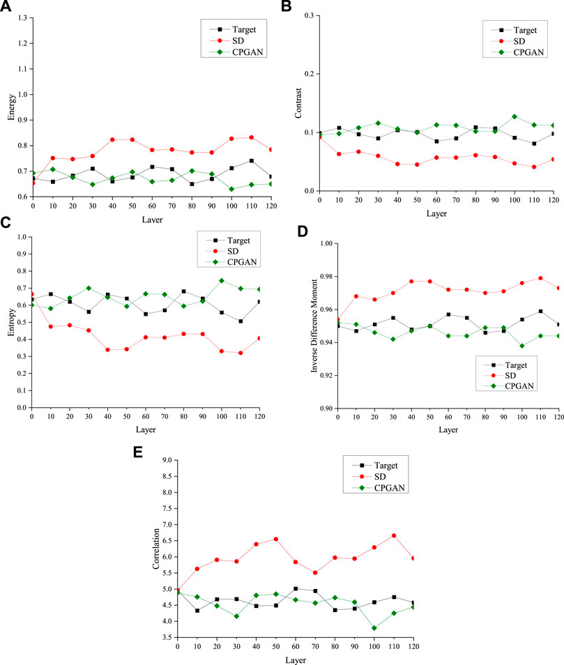
FIGURE 8. Comparison of characteristic functions of structures reconstructed by different algorithms: (A) energy; (B) contrast; (C) entropy; (D) inverse difference moment; and (E) correlation.

4.4.4 Pore Network Model and Seepage Analysis

The 3D reconstruction aims to use the reconstructed structure to analyze the seepage characteristics and other physical characteristics. The seepage characteristics mainly depend on the pore space characteristics and core connectivity characteristics, as well as many other complex factors. Therefore, the seepage experiment can be used to test whether the reconstructed structure has pore space characteristics similar to those of the target sample.

The pore network model is a common tool used for simulating the two-phase seepage characteristics of complex 3D core structures. Here, we used the maximum–minimum ball algorithm to extract pores and throats from core images. The essence of this algorithm is to extract the pore structure inside the core from the actual CT sequence of the core. Dividing pores and throats, their positions, link relationships, and other information reflects the morphological information and topological structure of the pores inside the core. Finally, the segmented pores and throats are abstracted as pipeline objects with different cross-sectional shapes, and dynamic displacement simulation research is carried out. In this study, we performed pore network extraction and seepage analysis on the reconstruction results based on this method.

After the pore network model was established, an oil–water two-phase seepage simulation experiment was carried out. The entire experiment included two stages: oil flooding (drainage) and water flooding (inhalation). To simulate the distribution of oil and water, assuming that the model is initially saturated with water, the oil flooding process simulation was carried out; that is, the wetting phase water was replaced with the non-wetting phase oil. After the process was completed, the middle of the hole contained non-wetting phase oil, while the corners were occupied by the wetting phase water. Water was injected from the inlet, and the water flooding simulation was performed to simulate the water flooding process in the actual formation.

Figures 9A–B shows the pore network model structure of the reference and reconstructed structures. Table 1 summarizes some important comparison parameters between the reconstructed and reference structures in the pore network model. Table 1 reports that the two sets of data are close in agreement, indicating that the pore space structures of the two 3D structures are similar.

FIGURE 9

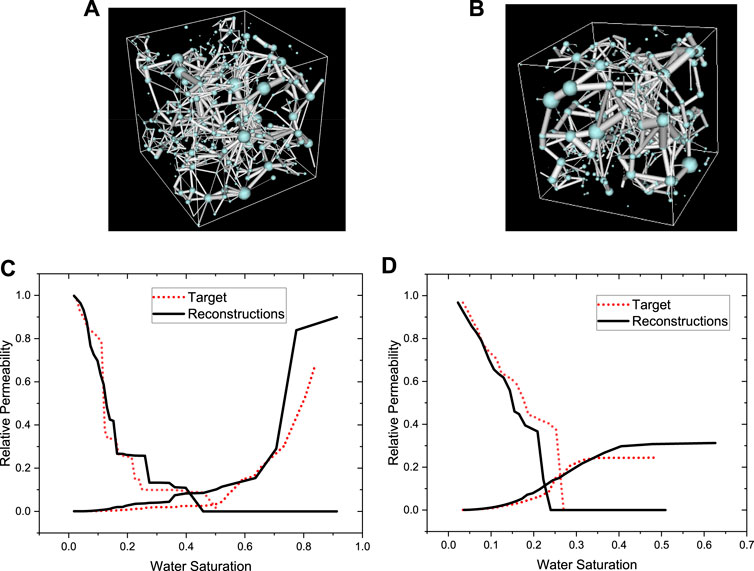
FIGURE 9. Pore network model and seepage experiment of the reconstructed structure and the target sample. (A) Pore network model of micro-CT image; (B) Pore network model of 3D reconstructed image; (C) oil flooding process; (D) water flooding process.

TABLE 1

TABLE 1. Comparison of the morphological parameters.

The experimental results of the seepage of the reconstructed structure and the target sample are also shown in Figure 9. Figures 9C, D shows the oil flooding process (drainage) and water flooding process (inhalation), respectively. As shown in the figure, the two-phase seepage curves, which have a strong dependence on the spatial structure, are also consistent. This shows from another perspective that the proposed algorithm can effectively reconstruct complex 3D structures.

4.4.5 Ablation Experiments

To verify the influence of the proposed and used loss functions on the reconstruction results, four comparative ablation experiments were conducted based on different combinations of loss functions (Table 2).

TABLE 2

TABLE 2. Loss function comparison experiment.

Table 3 presents an analysis of the evaluation function error between the reconstruction results using the four loss function combinations and the target 3D structure. The following equation was used to calculate the reconstruction error:

$error={\displaystyle \sum _r\left|f_{reconstruction}\left(r\right)-f_{t\arg et}\left(r\right)\right|}(20)$

TABLE 3

TABLE 3. Comparison of the reconstruction results. a) Two-point correlation function; (b) Linear path function; (c) Two-point cluster function; (d) Local porosity distribution. Each error is the average of 20 reconstruction results.

As summarized in Table 3, four evaluation functions were adopted. The two-point correlation function S₂(r) represents the correlation of the spatial distribution of two points, that is, the probability that two points belong to the same phase (pixel); the two-point cluster function L(r) is an important function describing the connectivity of porous media. Clusters refer to individual connected regions in the image. The two-point cluster function focuses on the probability that two points belong to the same cluster; the linear path function C₂(r) represents the probability that a line segment is completely contained by a cluster. The local porosity indicates the probability that the porosity of the measurement unit is within the specified range.

A trend of the overall reconstruction accuracy can be seen from the four parameters: the more the loss function is used, the higher the reconstruction accuracy.

In addition, the error obtained when using the original BicycleGAN loss alone is the largest. Based on the original BicycleGAN loss, the increase in the use of L_{grayscale pattern} alone can better improve the reconstruction accuracy compared to using the L_{grayscale pixel value} alone. Increasing the simultaneous use of L_{grayscale pattern} and L_{grayscale pixel value} can help achieve the smallest reconstruction error.

We further analyzed the local porosity distribution results described in Table 3. In the local porosity distribution, the peak reflects the maximum probability value of the porosity distribution. By calculation, in the 20 sets of repeated results in experiments 1-4, the mean and standard deviation of the porosity corresponding to the peak were 0.120 ± 0.022, 0.141 ± 0:015, 0.148 ± 0:012, 0.176 ± 0.010 (Mean ± Standard Deviation), separately. The porosity corresponding to the peak of the target sample is 0.171, which is the closest to the result of experiment 4. This indicates from another aspect that the 3D pore space distribution of the reconstructed structure in experiment 4 is the most similar to the target system.

4.4.6 Additional Performance Analysis of the Reconstruction Results

In the experiment, the test objects are core samples from the supplementary materials of the paper “Segmentation of digital rock images using deep convolutional autoencoder networks” by Sadegh Karimpoulia and Pejman Tahmasebi [56] (3D μCT image of Berea sandstone with a size of 1,024 × 1,024 × 1,024 voxels and a resolution of 0.74 μm). Figure 10B shows the 3D CT image of the real core, Figure 10C shows the reconstruction result, and Figure 10A) is the slice image of the input sample, which was randomly extracted from the core sample in Figure 10B for reconstruction.

FIGURE 10

FIGURE 10. Visual comparison between our reconstructions and the target. (A) reference image; (B) target system; (C) reconstruction structure.

From the perspective of visual effects, the reconstruction results had relatively similar grayscale and structural features to the real 3D structure, and the sizes of the pores and particles were relatively similar.

Figure 11A shows the benchmark samples of Berea sandstone detected in a scanning electron microscopy, which was mainly composed of quarts and K-feldspar. Figure 11B shows the related μCT image, from which the reconstruction experiments are done.

FIGURE 11

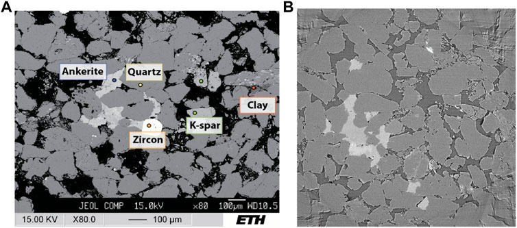
FIGURE 11. (A) Different minerals of Berea sandstone detected in a Scanning electron microscopy and (B) μCT image of Berea sandstone.

We tested the volume fraction, linear path function, and chord length distribution of different mineral compositions of the target system and reconstructed structures through repeating the experiments 20 times. In the target system and reconstructed structure, the average volume fractions of feldspar were 0.0524805 and 0.0627785 and of quartz were 0.760586 and 0.735257, respectively. Mineral composition distributions in the two 3D structures were very close, indicating that the algorithm proposed in this paper can reproduce the composition information of the structures to be reconstructed. The linear path function describes the connectivity of pores in the form of line segments. As shown in Figures 12A–B, the reconstructed structure is in good agreement with the reference structure linear path function. This shows that the algorithm can control the spatial distribution of mineral components in the 3D structure well, making this spatial distribution conform to the reference structure.

FIGURE 12

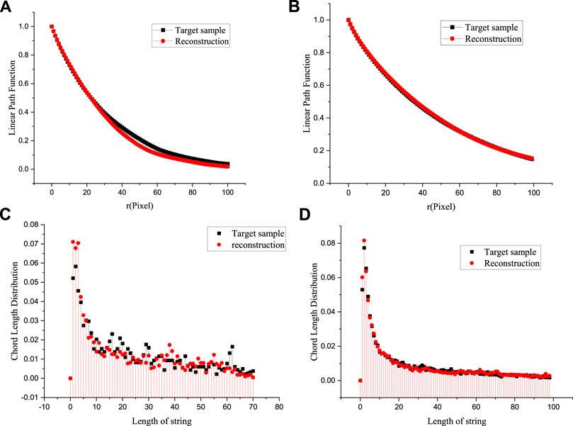
FIGURE 12. Comparison of linear path function (A–B) and chord length distribution function(C–D) between target systems and reconstructed structures for different mineral compositions.

The chord length distribution function of a certain phase of the structure is defined as

$F\left(C\right)=\frac{\overline{\ell \left(C\right)\times N\left(C\right)}}{\varphi }(21)$

Here $C$ represents the chord of the image, $\ell \left(C\right)$ the chord length of the chord, $N\left(C\right)$ the number of occurrences of the chord, and $\varphi$ the overall proportion of a certain phase. For example, when studying the porosity phase, $\varphi$ is the porosity, and $\overline{•}$ represents the overall statistical average. The results of the statistical analysis in Figures 12C–D showed that the chord length distribution functions of the same mineral components of the reconstructed structure and the reference structure have good consistency, that is, these components have similar morphological characteristics as a whole.

5 Conclusion

Here, we proposed a novel CPGAN model and related algorithms for the reconstruction of gray cores. This is achieved by combining the deep learning method with the idea of dimension enhancement in the SD frame. This network sets the input and target as 3D equivalent structures and learns the spatial structure of the gray core image through a 3D convolution kernel and the cascading of individual networks. In addition, we designed loss functions based on grayscale pixel distribution and grayscale pattern distribution for the training process of the network. We conducted experiments to reveal that gray core images reconstructed by CPGAN matched the target system very well. Comparing with the original SD reconstruction algorithm, we revealed that the proposed algorithm could better reconstruct the gray core image.

In summary, CPGAN is a flexible machine-learning framework for predicting gray level distribution and for maintaining the continuity and variability of reconstructed structures. The framework provides the reconstruction of 3D structures from 2D slices for gray level cores with different structure types and compositions. As an example of knowledge extraction, we applied this method to the design of a 3D core and showed that its design results were consistent with the structural characteristics of the target core. Moreover, the reconstruction time was significantly reduced compared to that of traditional algorithms.

Data Availability Statement

The data analyzed in this study is subject to the following licenses/restrictions: The data that has been used is confidential. Requests to access these datasets should be directed to mongli1989@163.com.

Author Contributions

YL designed experiments and wrote the article; PJ modified the article; GH collected samples.

Funding

This work was supported by the National Natural Science Foundation of China (Grant No. 61901533 and No. 61207014), Henan Province Science Foundation for Youths (No. 212300410197), and supported by the Key R & D and Promotion Projects of Henan Province (No. 212102210147).

Conflict of Interest

The authors declare that the research was conducted in the absence of any commercial or financial relationships that could be construed as a potential conflict of interest.

Publisher’s Note

All claims expressed in this article are solely those of the authors and do not necessarily represent those of their affiliated organizations, or those of the publisher, the editors, and the reviewers. Any product that may be evaluated in this article, or claim that may be made by its manufacturer, is not guaranteed or endorsed by the publisher.

Acknowledgments

The authors thank Heiko Andrä of Fraunhofer ITWM, Germany, Claudio Madonna at ETH Zurich, Department of Earth Sciences, Zurich, Switzerland and Sadegh Karimpouli at the Department of Mining Engineering Group, Faculty of Engineering, University of Zanjan for providing several images of porous media used in this work. The authors also would like to thank the constructive comments from reviewers and the associate editor that helped us to improve the manuscript.

Supplementary Material

The Supplementary Material for this article can be found online at: https://www.frontiersin.org/articles/10.3389/fphy.2022.716708/full#supplementary-material

References

1. Ju Y, Huang Y, Gong W, Zheng J, Xie H, Wang L, et al. 3-D Reconstruction Method for Complex Pore Structures of Rocks Using a Small Number of 2-D X-Ray Computed Tomography Images. IEEE Trans Geosci Remote Sensing (2019) 57(4):1873–82. doi:10.1109/tgrs.2018.2869939

CrossRef Full Text | Google Scholar

2. Bostanabad R, Zhang Y, Li X, Kearney T, Brinson LC, Apley DW, et al. Computational Microstructure Characterization and Reconstruction: Review of the State-Of-The-Art Techniques. Prog Mater Sci (2018) 95:1–41. doi:10.1016/j.pmatsci.2018.01.005

CrossRef Full Text | Google Scholar

3. Li H, Singh S, Chawla N, Jiao Y. Direct Extraction of Spatial Correlation Functions from Limited X-ray Tomography Data for Microstructural Quantification. Mater Characterization (2018) 140:265–74. doi:10.1016/j.matchar.2018.04.020

CrossRef Full Text | Google Scholar

4. Wang Y, Arns J-Y, Rahman SS, Arns CH. Three-dimensional Porous Structure Reconstruction Based on Structural Local Similarity via Sparse Representation on Micro-computed-tomography Images. Phys Rev E (2018) 98(4):043310. doi:10.1103/physreve.98.043310

CrossRef Full Text | Google Scholar

5. Tahmasebi P, Javadpour F, Sahimi M. Three-Dimensional Stochastic Characterization of Shale SEM Images. Transp Porous Media (2015) 110(3):1–11. doi:10.1007/s11242-015-0570-1

CrossRef Full Text | Google Scholar

6. Zhang W, Song L, Li J. Efficient 3D Reconstruction of Random Heterogeneous media via Random Process Theory and Stochastic Reconstruction Procedure. Comp Methods Appl Mech Eng (2019) 354:1–15. doi:10.1016/j.cma.2019.05.033

CrossRef Full Text | Google Scholar

7. Lamine S, Edwards MG. Multidimensional Upwind Schemes and Higher Resolution Methods for Three-Component Two-phase Systems Including Gravity Driven Flow in Porous media on Unstructured Grids. Comp Methods Appl Mech Eng (2015) 292:171–94. doi:10.1016/j.cma.2014.12.022

CrossRef Full Text | Google Scholar

8. Kalukin AR, Van Geet M, Swennen R. Principal Components Analysis of Multienergy X-ray Computed Tomography of mineral Samples. IEEE Trans Nucl Sci (2000) 47(5):1729–36. doi:10.1109/23.890998

CrossRef Full Text | Google Scholar

9. Guo X, Zou G, Wang Y, Wang Y, Gao T. Investigation of the Temperature Effect on Rock Permeability Sensitivity. J Pet Sci Eng (2017) 156:616–22. doi:10.1016/j.petrol.2017.06.045

CrossRef Full Text | Google Scholar

10. Zhu SY, Du ZM, Li CL, Salmachi A, Peng XL, Wang CW, et al. A Semi-analytical Model for Pressure-dependent Permeability of Tight Sandstone Reservoirs. Transport Porous Med (2018) 122(2):1–18. doi:10.1007/s11242-018-1001-x

CrossRef Full Text | Google Scholar

11. Munawar MJ, Lin C, Cnudde V, Bultreys T, Dong C, Zhang X, et al. Petrographic Characterization to Build an Accurate Rock Model Using micro-CT: Case Study on Low-Permeable to Tight Turbidite sandstone from Eocene Shahejie Formation. Micron (2018) 109:22–33. doi:10.1016/j.micron.2018.02.010

PubMed Abstract | CrossRef Full Text | Google Scholar

12. Suehiro S, Ohta K, Hirose K, Morard G, Ohishi Y. The Influence of Sulfur on the Electrical Resistivity of Hcp Iron: Implications for the Core Conductivity of Mars and Earth. Geophys Res Lett (2017) 44(16):8254–9. doi:10.1002/2017gl074021

CrossRef Full Text | Google Scholar

13. Bayrakci G, Falcon-Suarez IH, Minshull TA, North L, Best AI. Anisotropic Physical Properties of Mafic and Ultramafic Rocks from an Oceanic Core Complex. Geochem Geophy Geosy (2018) 19(11). doi:10.1029/2018gc007738

CrossRef Full Text | Google Scholar

14. Li Y, Yang X, Yu JH, Cai YF. Unusually High Electrical Conductivity of Phlogopite: the Possible Role of Fluorine and Geophysical Implications. Contrib Mineral Petr (2016) 171(4):1–11. doi:10.1007/s00410-016-1252-x

CrossRef Full Text | Google Scholar

15. Chekhonin E, Popov E, Popov Y, Gabova A, Romushkevich R, Spasennykh M, et al. High-Resolution Evaluation of Elastic Properties and Anisotropy of Unconventional Reservoir Rocks via Thermal Core Logging. Rock Mech Rock Eng (2018) 51(9):2747–59. doi:10.1007/s00603-018-1496-z

CrossRef Full Text | Google Scholar

16. Sone H, Zoback MD. Mechanical Properties of Shale-Gas Reservoir Rocks — Part 2: Ductile Creep, Brittle Strength, and Their Relation to the Elastic Modulus. Geophysics (2013) 78(5):D390–D399. doi:10.1190/geo2013-0051.1

CrossRef Full Text | Google Scholar

17. Piasta W, Góra J, Budzyński W. Stress-strain Relationships and Modulus of Elasticity of Rocks and of Ordinary and High Performance Concretes. Construction Building Mater (2017) 153:728–39. doi:10.1016/j.conbuildmat.2017.07.167

CrossRef Full Text | Google Scholar

18. Muljadi BP, Blunt MJ, Raeini AQ, Bijeljic B. The Impact of Porous media Heterogeneity on Non-darcy Flow Behaviour from Pore-Scale Simulation. Adv Water Resour (2016) 95:329–40. doi:10.1016/j.advwatres.2015.05.019

CrossRef Full Text | Google Scholar

19. Yan C, Zheng H. FDEM-flow3D: A 3D Hydro-Mechanical Coupled Model Considering the Pore Seepage of Rock Matrix for Simulating Three-Dimensional Hydraulic Fracturing. Comput Geotechnics (2017) 81:212–28. doi:10.1016/j.compgeo.2016.08.014

CrossRef Full Text | Google Scholar

20. Nash S, Rees DAS. The Effect of Microstructure on Models for the Flow of a Bingham Fluid in Porous Media: One-Dimensional Flows. Transp Porous Med (2017) 116(3):1073–92. doi:10.1007/s11242-016-0813-9

CrossRef Full Text | Google Scholar

21. Vilcáez J, Morad S, Shikazono N. Pore-scale Simulation of Transport Properties of Carbonate Rocks Using FIB-SEM 3D Microstructure: Implications for Field Scale Solute Transport Simulations. J Nat Gas Sci Eng (2017) 42:13–22.

Google Scholar

22. Zhang J, Ma G, Ming R, Cui X, Li L, Xu H. Numerical Study on Seepage Flow in Pervious concrete Based on 3D CT Imaging. Construction Building Mater (2018) 161:468–78. doi:10.1016/j.conbuildmat.2017.11.149

CrossRef Full Text | Google Scholar

23. Zhang Y, Lebedev M, Jing Y, Yu H, Iglauer S. In-situ X-ray Micro-computed Tomography Imaging of the Microstructural Changes in Water-Bearing Medium Rank Coal by Supercritical CO2 Flooding. Int J Coal Geology (2019) 203:28–35. doi:10.1016/j.coal.2019.01.002

CrossRef Full Text | Google Scholar

24. Zhang Y, Lebedev M, Al-Yaseri A, Yu H, Xu X, Sarmadivaleh M, et al. Nanoscale Rock Mechanical Property Changes in Heterogeneous Coal after Water Adsorption. Fuel (2018) 218:23–32. doi:10.1016/j.fuel.2018.01.006

CrossRef Full Text | Google Scholar

25. Bouchelaghem F, Pusch R. Fluid Flow and Effective Conductivity Calculations on Numerical Images of Bentonite Microstructure. Appl Clay Sci (2017) 144:9–18. doi:10.1016/j.clay.2017.04.023

CrossRef Full Text | Google Scholar

26. Bai B, Elgmati M, Zhang H, Wei M. Rock Characterization of Fayetteville Shale Gas Plays. Fuel (2013) 105:645–52. doi:10.1016/j.fuel.2012.09.043

CrossRef Full Text | Google Scholar

27. Pejman T, Muhammad S. A Stochastic Multiscale Algorithm for Modeling Complex Granular Materials. Granul Matter (2018) 20(3):45.

Google Scholar

28. Yeong S, Torquato CLY. Reconstructing Random media. Phys Rev E (1998) 57(1):495–506.

CrossRef Full Text | Google Scholar

29. Yeong CLY, Torquato S. Reconstructing Random Media: II, Three-Dimensional Media from Two-Dimensional Cuts. Phys Rev E (1998) 58(1). doi:10.1103/physreve.58.224

CrossRef Full Text | Google Scholar

30. Izadi H, Baniassadi M, Hasanabadi A, Mehrgini B, Memarian H, Soltanian-Zadeh H, et al. Application of Full Set of Two point Correlation Functions from a Pair of 2D Cut Sections for 3D Porous media Reconstruction. J Pet Sci Eng (2017) 149:789–800. doi:10.1016/j.petrol.2016.10.065

CrossRef Full Text | Google Scholar

31. Okabe H, Blunt MJ. Pore Space Reconstruction Using Multiple-point Statistics. J Petrol Sci Eng (2005) 46(1):121–37. doi:10.1016/j.petrol.2004.08.002

CrossRef Full Text | Google Scholar

32. Liang ZR, Fernandes CP, Magnani FS, Philippi PC. A Reconstruction Technique for Three-Dimensional Porous media Using Image Analysis and Fourier Transforms. J Pet Sci Eng (1998) 21:273–83. doi:10.1016/s0920-4105(98)00077-1

CrossRef Full Text | Google Scholar

33. Xiaohai H, Yang L, Qizhi T, Zhengji L, Linbo Q. Learning-based Super-dimension (SD) Reconstruction of Porous media from a Single Two-Dimensional Image. In: 2016 IEEE International Conference on Signal Processing, Communications and Computing (ICSPCC) (2016). doi:10.1109/icspcc.2016.7753653

CrossRef Full Text | Google Scholar

34. Li Y, He X, Teng Q, Feng J, Wu X. Markov Prior-Based Block-Matching Algorithm for Superdimension Reconstruction of Porous media. Phys Rev E (2018) 97(4):043306. doi:10.1103/PhysRevE.97.043306

PubMed Abstract | CrossRef Full Text | Google Scholar

35. Li Y, Teng Q, He X, Feng J, Xiong S. Super-dimension-based Three-Dimensional Nonstationary Porous Medium Reconstruction from Single Two-Dimensional Image. J Pet Sci Eng (2019) 174:968–83. doi:10.1016/j.petrol.2018.12.004

CrossRef Full Text | Google Scholar

36. Li Y, Teng Q, He X, Ren C, Chen H, Feng J. Dictionary Optimization and Constraint Neighbor Embedding-Based Dictionary Mapping for Superdimension Reconstruction of Porous media. Phys Rev E (2019) 99(6):062134. doi:10.1103/PhysRevE.99.062134

PubMed Abstract | CrossRef Full Text | Google Scholar

37. Freeman WT, Jones W, Jones TR, Pasztor EC. Example-Based Super-resolution. IEEE Comput Grap Appl (2002) 22(2):56–65. doi:10.1109/38.988747

CrossRef Full Text | Google Scholar

38. Mishra D, Majhi B, Sa PK, Dash R. Development of Robust Neighbor Embedding Based Super-resolution Scheme. Neurocomputing (2016) 202(19):49–66. doi:10.1016/j.neucom.2016.04.013

CrossRef Full Text | Google Scholar

39. Kumar N, Sethi A. Fast Learning-Based Single Image Super-resolution. IEEE Trans Multimedia (2016) 18(8):1504–15. doi:10.1109/tmm.2016.2571625

CrossRef Full Text | Google Scholar

40. Sandeep P, Jacob T. Single Image Super-resolution Using a Joint GMM Method. IEEE Trans Image Process (2016) 25(9):4233–44. doi:10.1109/TIP.2016.2588319

PubMed Abstract | CrossRef Full Text | Google Scholar

41. Feng J, Teng Q, He X, Wu X. Accelerating Multi-point Statistics Reconstruction Method for Porous media via Deep Learning. Acta Materialia (2018) 159:296–308. doi:10.1016/j.actamat.2018.08.026

CrossRef Full Text | Google Scholar

42. Mosser L, Dubrule O, Blunt MJ. Reconstruction of Three-Dimensional Porous media Using Generative Adversarial Neural Networks. Phys Rev E (2017) 96(4):043309. doi:10.1103/PhysRevE.96.043309

PubMed Abstract | CrossRef Full Text | Google Scholar

43. Mosser L, Dubrule O, Blunt MJ. Conditioning of Three-Dimensional Generative Adversarial Networks for Pore and Reservoir-Scale Models. In: 80th EAGE Conference and Exhibition (2018).

Google Scholar

44. Mosser L, Dubrule O, Blunt MJ. Stochastic Reconstruction of an Oolitic Limestone by Generative Adversarial NetworksTransp Porous Med (2018) 125. New York, NY, USA: Springer p. 81–103. doi:10.1007/s11242-018-1039-9

CrossRef Full Text | Google Scholar

45. Sermanet P, Kavukcuoglu K, Chintala S, Lecun Y. Pedestrian Detection with Unsupervised Multi-Stage Feature Learning. In: 2013 IEEE Conference on Computer Vision and Pattern Recognition (2013). p. 3626–33. doi:10.1109/cvpr.2013.465

CrossRef Full Text | Google Scholar

46. Chong E, Han C, Park FC. Deep Learning Networks for Stock Market Analysis and Prediction: Methodology, Data Representations, and Case Studies. Expert Syst Appl (2017) 83:187–205. doi:10.1016/j.eswa.2017.04.030

CrossRef Full Text | Google Scholar

47. Feng J, Teng Q, Li B, He X, Chen H, Li Y. An End-To-End Three-Dimensional Reconstruction Framework of Porous media from a Single Two-Dimensional Image Based on Deep Learning. Comp Methods Appl Mech Eng (2020) 368:113043. doi:10.1016/j.cma.2020.113043

CrossRef Full Text | Google Scholar

48. Laloy E, Hérault R, Lee J, Jacques D, Linde N. Inversion Using a New Low-Dimensional Representation of Complex Binary Geological media Based on a Deep Neural Network. Adv Water Resour (2017) 110:387–405. doi:10.1016/j.advwatres.2017.09.029

CrossRef Full Text | Google Scholar

49. Laloy E, Hérault R, Jacques D, Linde N. Training‐Image Based Geostatistical Inversion Using a Spatial Generative Adversarial Neural Network. Water Resour Res (2018) 54(1):381–406. doi:10.1002/2017wr022148

CrossRef Full Text | Google Scholar

50. Zhu J-Y, Zhang R, Pathak D, Darrell T, Efros AA, Wang O, et al. Toward Multimodal Image-To-Image Translation. In: Proc. Proceedings of the 31st International Conference on Neural Information Processing Systems. California, USA: Long Beach (2017). p. 465–76.

Google Scholar

51. Isola P, Zhu J, Zhou T, Efros AA. Image-to-Image Translation with Conditional Adversarial Networks. In: 2017 IEEE Conference on Computer Vision and Pattern Recognition (CVPR) (2017). p. 5967–76. doi:10.1109/cvpr.2017.632

CrossRef Full Text | Google Scholar

52. Wu A, Zheng W, Yu H, Gong S, Lai J. RGB-infrared Cross-Modality Person Re-identification. In: 2017 IEEE International Conference on Computer Vision (ICCV) (2017). p. 5390–9. doi:10.1109/iccv.2017.575

CrossRef Full Text | Google Scholar

53. Biswal B, Manwart C, Hilfer R. Three-dimensional Local Porosity Analysis of Porous media. Physica A (1998) 255(3-4):221–41. doi:10.1016/s0378-4371(98)00111-3

CrossRef Full Text | Google Scholar

54. Hu J, Stroeven P. Local Porosity Analysis of Pore Structure in Cement Paste. Cement Concrete Res (2005) 35(2):233–42. doi:10.1016/j.cemconres.2004.06.018

CrossRef Full Text | Google Scholar

55. Ding K, Ma K, Wang S, Simoncel li EP. Image Quality Assessment: Unifying Structure an and Texture Similarity. In: IEEE Transactions on Pattern Analysis and Machine Intelligence (2020).

Google Scholar

56. Karimpouli S, Tahmasebi P. Segmentation of Digital Rock Images Using Deep Convolutional Autoencoder Networks. Comput Geosciences (2019) 126(MAY):142–50. doi:10.1016/j.cageo.2019.02.003

CrossRef Full Text | Google Scholar