Approximate solutions to shallow water wave equations by the homotopy perturbation method coupled with Mohand transform

In this paper, the Mohand transform-based homotopy perturbation method is proposed to solve two-dimensional linear and non-linear shallow water wave equations. This approach has been proved suitable for a broad variety of non-linear differential equations in science and engineering. The variation trend of the water surface elevation at different time levels and depths are given by some graphs. Moreover, the obtained solutions are compared with the existing results, which show higher efficiency and fewer computations than other approaches studied in the literature.

1 Introduction

Water waves that have a horizontal scale much larger than the depth of the fluid are considered shallow water waves (SWWs). SWWs describe the evolution of incompressible flow, neglecting density change along the depth, which are widely used to simulate the propagation of tsunami waves, tidal currents, storm floods, and shock waves [1–5]. Karunakar and Chakraverty applied the homotopy perturbation method (HPM) to solve linear and non-linear one-dimensional shallow water wave equations (SWWEs) [1], while the two-dimensional equations were solved in [6]. Sahoo and Chakraverty [7] used the Sawi transform-based homotopy perturbation method to solve the one-dimensional SWWEs. The application of the variational iteration method and homotopy perturbation method (HPM) was given in [8] for solving one-dimensional shallow water equations with crisp and fuzzy uncertain initial conditions. Noeiaghdam and Sidorov [9] used the homotopy analysis method to solve the non-linear shallow water wave equation. Safari [10] gave solutions to two extended model equations for shallow water waves by He’s variational iteration method. In [11], the Adomian decomposition method was used to solve two extended model equations for SWWEs. In addition, Bekir and Aksoy [12] applied the Exp-function method to construct exact solutions to non-linear wave equations.

Mohand transform (MT) [13] is an integral transformation, which is obtained from the classical Fourier integral, and it was initiated by Mohand Mahgoub to solve some integral and differential equations (14–16). Khandelwal [17] combined the Adomian decomposition method and Mohand transform for solving a differential equation of mixing layers that arise in a viscous incompressible form. The comparison of two integral transforms between Mohand and Laplace is given in [18]; the results show that the two transforms are closely related. Aggarwal, Sharma, and Chauhan [19] gave the duality relations of Kamal transform with Laplace, Laplace−Carson, Aboodh, Sumudu, Elzaki, Mohand, and Sawi transforms [20]. They used an effective scheme based on Mohand transform and the homotopy perturbation method to find numerical solutions to non-linear fractional shock wave equations. Althobaiti, Dubey, and Prasad [21] presented the local fractional Mohand transform with the Adomian decomposition method to solve the local fractional generalized Fokker–Planck equation. Shah, Khan, and Farooq et al. [22] employed the Mohand transform to provide the analytical solution to the one-dimensional time fractional system of PDEs.

The homotopy perturbation method (HPM) [23] has been widely used for solving differential and integral equations, which was first proposed and developed by the Chinese mathematician Ji-Huan He [24–28]. Laplace transformation coupled with the homotopy perturbation method is called the He−Laplace method. Madani and Mishra [29, 30] adopted this method to solve non-linear ordinary and partial differential equations. It is proved that this method needs fewer computations and is much easier than other methods. He, Moatimid, and Zekry [31] used the two-scale transforms and He−Laplace method to get an analytic approximate solution to a fractal−differential model [32]. They presented the combination of the enhanced perturbation method and the parameter expansion technology based on Li−He’s approach, aiming to find an approximate solution to the given second-order non-linear ordinary differential equation [33]. They applied the basic idea of the perturbation method to construct a homotopy equation with a higher order; the results show a highly effective obtained solution. The approximation of the damped non-linear Klein–Gordon equation was given [34] by the coupling of the exponential decay parameter with the homotopy perturbation method, which overcomes the shortcomings of the classical method [35]. They used the reducing rank method with the homotopy perturbation method to solve the third-order Duffing equation.

The main purpose of the present work is to solve two-dimensional linear and non-linear shallow water wave equations by coupling Mohand transform with the homotopy perturbation method. The remainder of the paper is organized as follows: in Section 2, we present some preliminaries about shallow water wave equations (SWWEs), Mohand transform (MT), and the homotopy perturbation method (HPM). In Section 3, the Mohand transform (MT)-based homotopy perturbation method (HPM) is applied to solve coupled linear and non-linear SWWEs in two dimensions. In Section 4, the variations in the water surface elevation have been demonstrated at different time levels and depths. Finally, conclusions have been drawn in Section 5.

2 Preliminaries

2.1 Shallow water wave equations (SWWEs)

The linear SWWEs in two dimensions [2, 3] may be given as follows:

$\begin{array}{l}\frac{\partial \eta }{\partial t}+\frac{\partial R}{\partial x}+\frac{\partial Q}{\partial y}=0\\ \frac{\partial R}{\partial t}+gh\frac{\partial \eta }{\partial x}=0\\ \frac{\partial Q}{\partial t}+gh\frac{\partial \eta }{\partial y}=0\end{array}(1)$

As such, the non-linear SWWEs [2, 3] may be written as

$\begin{array}{l}\frac{\partial \eta }{\partial t}+\frac{\partial R}{\partial x}+\frac{\partial Q}{\partial y}=0\\ \frac{\partial R}{\partial t}+g\left(h+\eta \right)\frac{\partial \eta }{\partial x}=0\\ \frac{\partial Q}{\partial t}+g\left(h+\eta \right)\frac{\partial \eta }{\partial y}=0\end{array}(2)$

where $\eta$ is the water surface elevation, $t$ is the time, $R$ and $Q$ are the depth-averaged volume flux in $x$ and $y$ directions, $g$ is the acceleration due to gravity $\left(g=9.8\right)$, and $h$ is the water depth.

2.2 Mohand transform (MT) and some of its properties

The Mohand transform of the function $w\left(t\right),t\ge 0$ is given by [13]

$M\left\{w\left(t\right)\right\}=u^2{\int }_0^{\infty }w\left(t\right)e^{-ut}dt=T\left(u\right)(3)$

Mohand transform of some useful fundamental functions is given in Table 1.

TABLE 1

TABLE 1. MT of frequently encountered functions.

The linearity property of MT is given as follows [15]: if $M\left\{w_1\left(t\right)\right\}=T_1\left(u\right),M\left\{w_2\left(t\right)\right\}=T_2\left(u\right)$, then $M\left\{l{w}_1\left(t\right)+m{w}_2\left(t\right)\right\}=lM\left\{w_1\left(t\right)\right\}+mM\left\{w_2\left(t\right)\right\}=l{T}_1\left(u\right)+m{T}_2\left(u\right)$, where $l$ and $m$ are the arbitrary constants.

Let $M\left\{w\left(x,t\right)\right\}=T\left(x,u\right)$; to obtain MT of a partial derivative, we use integration by parts, and then we derive the following [15]:

$\begin{array}{l}M\left\{\frac{\partial w\left(x,t\right)}{\partial t}\right\}=uT\left(x,u\right)-u^{2}w\left(x,0\right),\\ M\left\{\frac{{\partial }^{2}w\left(x,t\right)}{\partial t^2}\right\}=u^{2}T\left(x,u\right)-u^{3}w\left(x,0\right)-u^2\frac{\partial w\left(x,0\right)}{\partial t}\\ M\left\{\frac{{\partial }^{n}w\left(x,t\right)}{\partial t^n}\right\}=u^{n}T\left(x,u\right)-{\displaystyle \sum }_{k=0}^{n-1}{u}^{n-k+1}\frac{{\partial }^{k}w\left(x,0\right)}{\partial t^k}.\end{array}(4)$

The function $w\left(t\right)$ is called the inverse Mohand transform of the function $T\left(u\right)$ if it has the following property: $M^{-1}\left[T\left(u\right)\right]=w\left(t\right)$. The inverse Mohand transform of some useful fundamental functions [15] is given in Table2.

TABLE 2

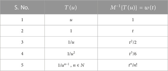
TABLE 2. Inverse MT of frequently encountered functions.

2.3 Homotopy perturbation method (HPM)

To illustrate the basic ideas of the HPM [19], we consider the following non-linear differential equation:

$A\left(u\right)-f\left(r\right)=0,r\in \mathrm{\Omega }(5)$

with the following boundary conditions:

$B\left(u,\partial u/\partial n\right)=0,r\in \mathrm{\Gamma }(6)$

Here, $A$ is a general differential operator, $B$ is a boundary operator, $f\left(r\right)$ is a known analytic function, and $\mathrm{\Gamma }$ is the boundary of the domain $\mathrm{\Omega }$.

The operator $A$ can be divided into two parts $L$ and $N$, where $L$ is linear and $N$ is non-linear; Eq. 5 can be rewritten as follows:

$L\left(u\right)+N\left(u\right)-f\left(r\right)=0(7)$

Using the homotopy technique, one may construct a homotopy $v\left(r,p\right):\mathrm{\Omega }\times \left[\mathrm{0,1}\right]\to R$, which satisfies the following:

$H\left(v,p\right)=\left(1-p\right)\left[L\left(u\right)-L\left(u_0\right)\right]+p\left[A\left(v\right)-f\left(r\right)\right]=0,p\in \left[\mathrm{0,1}\right](8)$

or

$H\left(v,p\right)=L\left(v\right)-L\left(u_0\right)+pL\left(u_0\right)+p\left[N\left(v\right)-f\left(r\right)\right]=0(9)$

where $p\in \left[\mathrm{0,1}\right]$ is an embedding parameter and $u_0$ is an initial approximation of Eq. 5, which satisfies the boundary conditions. Evidently, from Eqs 8, 9, we obtain the following:

$\begin{array}{l}H\left(v,0\right)=L\left(v\right)-L\left(u_0\right)=0\\ H\left(v,1\right)=A\left(v\right)-f\left(r\right)=0\end{array}(10)$

The changing process of $p$ from zero to unity is same as that of $v\left(r,p\right)$ from $u_0\left(r\right)$ to $u\left(r\right)$. In topology, this is called deformation, and $L\left(v\right)-L\left(u_0\right)$ and $A\left(v\right)-f\left(r\right)$ are called homotopic functions.

We consider the solution to Eq. 8 as a power series in $p\in \left[\mathrm{0,1}\right]$, given as follows:

$v=v_0+p{v}_1+p^2{v}_2+\cdots (11)$

The approximate solution to Eq. 5 will be obtained by substituting $p=1$ in Eq. 11.

$u=\underset{p\to 1}{\lim }v=v_0+v_1+v_2+\cdots (12)$

3 Approximate solutions to shallow water wave equations using the Mohand transform-based homotopy perturbation method (MHPM)

3.1 Linear shallow water wave equations

In this section, we obtain the series solution to linear two-dimensional shallow water Eq. 1 by the MHPM.

Let us consider the Gaussian initial conditions for $\eta ,R$ and Q, given as follows:

$\begin{array}{l}\eta \left(x,y,0\right)=0.5e^{-\frac{{\left(x-20\right)}^2}{10}-\frac{{\left(y-20\right)}^2}{20}}\\ R\left(x,y,0\right)=50e^{-\frac{{\left(x-20\right)}^2}{10}-\frac{{\left(y-20\right)}^2}{20}}\\ Q\left(x,y,0\right)=50e^{-\frac{{\left(x-20\right)}^2}{10}-\frac{{\left(y-20\right)}^2}{20}}\end{array}(13)$

Applying Mohand transform in Eq. 1, we obtain

$M\left\{\frac{\partial \eta }{\partial t}\right\}+M\left\{\frac{\partial R}{\partial x}\right\}+M\left\{\frac{\partial Q}{\partial y}\right\}=0(14)$

$M\left\{\frac{\partial R}{\partial t}\right\}+M\left\{gh\frac{\partial \eta }{\partial x}\right\}=0(15)$

$M\left\{\frac{\partial Q}{\partial t}\right\}+M\left\{gh\frac{\partial \eta }{\partial y}\right\}=0(16)$

Using the derivative characteristics of Mohand transform, Eq. 14 may be written as

$M\left\{\eta \left(x,y,t\right)\right\}=0.5u{e}^{-\frac{{\left(x-20\right)}^2}{10}-\frac{{\left(y-20\right)}^2}{20}}-\frac{1}{u}M\left\{\frac{\partial R\left(x,y,t\right)}{\partial x}\right\}-\frac{1}{u}M\left\{\frac{\partial Q\left(x,y,t\right)}{\partial y}\right\}(17)$

Taking the inverse of Mohand transform on both sides of Eq. 17, we may obtain the following:

$\eta \left(x,y,t\right)=0.5e^{-\frac{{\left(x-20\right)}^2}{10}-\frac{{\left(y-20\right)}^2}{20}}-M^{-1}\left[\frac{1}{u}M\left\{\frac{\partial R\left(x,y,t\right)}{\partial x}\right\}\right]-M^{-1}\left[\frac{1}{u}M\left\{\frac{\partial Q\left(x,y,t\right)}{\partial y}\right\}\right](18)$

Similarly, on solving Eqs 15, 16 by applying the same aforementioned procedure, we may obtain

$R\left(x,y,t\right)=50e^{-\frac{{\left(x-20\right)}^2}{10}-\frac{{\left(y-20\right)}^2}{20}}-M^{-1}\left[\frac{1}{u}M\left\{gh\frac{\partial \eta \left(x,y,t\right)}{\partial x}\right\}\right](19)$

$Q\left(x,y,t\right)=50e^{-\frac{{\left(x-20\right)}^2}{10}-\frac{{\left(y-20\right)}^2}{20}}-M^{-1}\left[\frac{1}{u}M\left\{gh\frac{\partial \eta \left(x,y,t\right)}{\partial y}\right\}\right](20)$

Now using the HPM technique, we may construct a homotopy for Eqs 18, 19, 20 in the following form:

$\begin{array}{l}\left(1-p\right)\left[\eta -{\eta }_0\right]+p\left[\eta -{\eta }_0+M^{-1}\left[\frac{1}{u}M\left\{\frac{\partial R}{\partial x}\right\}\right]+M^{-1}\left[\frac{1}{u}M\left\{\frac{\partial Q}{\partial y}\right\}\right]\right]=0\\ \left(1-p\right)\left[R-R_0\right]+p\left[R-R_0+M^{-1}\left[\frac{1}{u}M\left\{\frac{\partial \eta }{\partial x}\right\}\right]\right]=0\\ \left(1-p\right)\left[Q-Q_0\right]+p\left[Q-Q_0+M^{-1}\left[\frac{1}{u}M\left\{\frac{\partial \eta }{\partial y}\right\}\right]\right]=0\end{array}(21)$

By simplifying the aforementioned formulas, we may obtain

$\begin{array}{l}\eta ={\eta }_0-p{M}^{-1}\left[\frac{1}{u}M\left\{\frac{\partial R}{\partial x}\right\}\right]-p{M}^{-1}\left[\frac{1}{u}M\left\{\frac{\partial Q}{\partial y}\right\}\right]\\ R=R_0-p{M}^{-1}\left[\frac{1}{u}M\left\{gh\frac{\partial \eta }{\partial x}\right\}\right]\\ Q=Q_0-p{M}^{-1}\left[\frac{1}{u}M\left\{gh\frac{\partial \eta }{\partial y}\right\}\right]\end{array}(22)$

Let us consider the solution to Eq. 1 in the power series form as:

$\begin{array}{l}\eta ={\eta }_0+p{\eta }_1+p^2{\eta }_2+\cdots \\ R=R_0+p{R}_1+p^2{R}_2+\cdots \\ Q=Q_0+p{Q}_1+p^2{Q}_2+\cdots \end{array}(23)$

we may get the following results by applying Eq. 23 in Eq. 22 and comparing the coefficients of $p^0$:

$\begin{array}{l}{\eta }_0=0.5e^{-\frac{{\left(x-20\right)}^2}{10}-\frac{{\left(y-20\right)}^2}{20}}\\ R_0=50e^{-\frac{{\left(x-20\right)}^2}{10}-\frac{{\left(y-20\right)}^2}{20}}\\ Q_0=50e^{-\frac{{\left(x-20\right)}^2}{10}-\frac{{\left(y-20\right)}^2}{20}}\end{array}(24)$

Comparing the coefficients of $p^1$ , we get

$\begin{array}{l}{\eta }_1=-M^{-1}\left[\frac{1}{u}M\left\{\frac{\partial R_0}{\partial x}\right\}\right]-M^{-1}\left[\frac{1}{u}M\left\{\frac{\partial Q_0}{\partial y}\right\}\right]\\ R_1=-M^{-1}\left[\frac{1}{u}M\left\{gh\frac{\partial {\eta }_0}{\partial x}\right\}\right]\\ Q_1=-M^{-1}\left[\frac{1}{u}M\left\{gh\frac{\partial {\eta }_0}{\partial y}\right\}\right]\end{array}(25)$

Similarly, comparing the coefficients of $p^2$ and $p^3$, we get

$\begin{array}{l}{\eta }_2=-M^{-1}\left[\frac{1}{u}M\left\{\frac{\partial R_1}{\partial x}\right\}\right]-M^{-1}\left[\frac{1}{u}M\left\{\frac{\partial Q_1}{\partial y}\right\}\right]\\ R_2=-M^{-1}\left[\frac{1}{u}M\left\{gh\frac{\partial {\eta }_1}{\partial x}\right\}\right]\\ Q_2=-M^{-1}\left[\frac{1}{u}M\left\{gh\frac{\partial {\eta }_1}{\partial y}\right\}\right]\end{array}(26)$

$\begin{array}{l}{\eta }_3=-M^{-1}\left[\frac{1}{u}M\left\{\frac{\partial R_2}{\partial x}\right\}\right]-M^{-1}\left[\frac{1}{u}M\left\{\frac{\partial Q_2}{\partial y}\right\}\right]\\ R_3=-M^{-1}\left[\frac{1}{u}M\left\{gh\frac{\partial {\eta }_2}{\partial x}\right\}\right]\\ Q_3=-M^{-1}\left[\frac{1}{u}M\left\{gh\frac{\partial {\eta }_2}{\partial y}\right\}\right]\end{array}(27)$

In the same way, by correlating the coefficients of $p^{n+1}$, we obtain the following generic pattern:

$\begin{array}{l}{\eta }_{n+1}=-M^{-1}\left[\frac{1}{u}M\left\{\frac{\partial R_n}{\partial x}\right\}\right]-M^{-1}\left[\frac{1}{u}M\left\{\frac{\partial Q_n}{\partial y}\right\}\right]\\ R_{n+1}=-M^{-1}\left[\frac{1}{u}M\left\{gh\frac{\partial {\eta }_n}{\partial x}\right\}\right]\\ Q_{n+1}=-M^{-1}\left[\frac{1}{u}M\left\{gh\frac{\partial {\eta }_n}{\partial y}\right\}\right]\end{array}(28)$

Finally, by performing MT on the right hand side of Eq. 25 and then taking inverse MT, at a constant depth $h=.1$, we obtain

$\begin{array}{l}{\eta }_1=\left[50\left(\frac{1}{5}x-4\right)+50\left(\frac{1}{10}y-2\right)\right]e^{-\frac{{\left(x-20\right)}^2}{10}-\frac{{\left(y-20\right)}^2}{20}}t\\ R_1=0.49\left(\frac{1}{5}x-4\right)e^{-\frac{{\left(x-20\right)}^2}{10}-\frac{{\left(y-20\right)}^2}{20}}t\\ Q_1=0.49\left(\frac{1}{10}y-2\right)e^{-\frac{{\left(x-20\right)}^2}{10}-\frac{{\left(y-20\right)}^2}{20}}t\end{array}(29)$

We can also get ${\eta }_2,{\eta }_3,\cdots$ by Eq. 28; the solution of Eq. 1 may be found in the following form:

$\eta ={\eta }_0+{\eta }_1+{\eta }_2+{\eta }_3+\cdots (30)$

3.2 Non-linear shallow water wave equations

In this section, we obtain the series solution to the non-linear shallow water wave equation in two-dimensional Eq. 2 using the MHPM with the same initial conditions in Eq. 24.

Applying the MT and HPM in Eq. 2, we may obtain

$\begin{array}{l}\eta ={\eta }_0-p{M}^{-1}\left[\frac{1}{u}M\left\{\frac{\partial R}{\partial x}\right\}\right]-p{M}^{-1}\left[\frac{1}{u}M\left\{\frac{\partial Q}{\partial y}\right\}\right]\\ R=R_0-p{M}^{-1}\left[\frac{1}{u}M\left\{g\left(h+\eta \right)\frac{\partial \eta }{\partial x}\right\}\right]\\ Q=Q_0-p{M}^{-1}\left[\frac{1}{u}M\left\{g\left(h+\eta \right)\frac{\partial \eta }{\partial y}\right\}\right]\end{array}(31)$

Here, we again consider the power series solution to Eq. 2 as in (Eq. 23). We may get the following results by substituting Eq. 23 in Eq. 31 and comparing the coefficients of $p^0$:

$\begin{array}{l}{\eta }_0=0.5e^{-\frac{{\left(x-20\right)}^2}{10}-\frac{{\left(y-20\right)}^2}{20}}\\ R_0=50e^{-\frac{{\left(x-20\right)}^2}{10}-\frac{{\left(y-20\right)}^2}{20}}\\ Q_0=50e^{-\frac{{\left(x-20\right)}^2}{10}-\frac{{\left(y-20\right)}^2}{20}}\end{array}(32)$

Comparing the coefficients of $p^1$, we get

$\begin{array}{l}{\eta }_1=-M^{-1}\left[\frac{1}{u}M\left\{\frac{\partial R_0}{\partial x}\right\}\right]-M^{-1}\left[\frac{1}{u}M\left\{\frac{\partial Q_0}{\partial y}\right\}\right]\\ R_1=-M^{-1}\left[\frac{1}{u}M\left\{g\left(h+{\eta }_0\right)+\frac{\partial {\eta }_0}{\partial x}\right\}\right]\\ Q_1=-M^{-1}\left[\frac{1}{u}M\left\{g\left(h+{\eta }_0\right)\frac{\partial {\eta }_0}{\partial y}\right\}\right]\end{array}(33)$

Similarly, comparing the coefficients of $p^2$, we get

$\begin{array}{l}{\eta }_2=-M^{-1}\left[\frac{1}{u}M\left\{\frac{\partial R_1}{\partial x}\right\}\right]-M^{-1}\left[\frac{1}{u}M\left\{\frac{\partial Q_1}{\partial y}\right\}\right]\\ R_2=-M^{-1}\left[\frac{1}{u}M\left\{g\left(\left(h+{\eta }_0\right),\frac{\partial {\eta }_1}{\partial x},+,{\eta }_1,\frac{\partial {\eta }_0}{\partial x}\right)\right\}\right]\\ Q_2=-M^{-1}\left[\frac{1}{u}M\left\{g\left(\left(h+{\eta }_0\right),\frac{\partial {\eta }_1}{\partial y},+,{\eta }_1,\frac{\partial {\eta }_0}{\partial y}\right)\right\}\right]\end{array}(34)$

By continuing to compare the coefficients of $p^3$, we get

$\begin{array}{l}{\eta }_3=-M^{-1}\left[\frac{1}{u}M\left\{\frac{\partial R_2}{\partial x}\right\}\right]-M^{-1}\left[\frac{1}{u}M\left\{\frac{\partial Q_2}{\partial y}\right\}\right]\\ R_3=-M^{-1}\left[\frac{1}{u}M\left\{g\left(\left(h+{\eta }_0\right),\frac{\partial {\eta }_2}{\partial x},+,{\eta }_1,\frac{\partial {\eta }_1}{\partial x},+,{\eta }_2,\frac{\partial {\eta }_0}{\partial x}\right)\right\}\right]\\ Q_3=-M^{-1}\left[\frac{1}{u}M\left\{g\left(\left(h+{\eta }_0\right),\frac{\partial {\eta }_2}{\partial y},+,{\eta }_1,\frac{\partial {\eta }_1}{\partial y},+,{\eta }_2,\frac{\partial {\eta }_0}{\partial y}\right)\right\}\right]\end{array}(35)$

By this way, comparing the coefficients of $p^{n+1}$, we get

$\begin{array}{l}{\eta }_{n+1}=-M^{-1}\left[\frac{1}{u}M\left\{\frac{\partial R_n}{\partial x}\right\}\right]-M^{-1}\left[\frac{1}{u}M\left\{\frac{\partial Q_n}{\partial y}\right\}\right]\\ R_{n+1}=-M^{-1}\left[\frac{1}{u}M\left\{g\left(\left(h+{\eta }_0\right),\frac{\partial {\eta }_n}{\partial x},+,{\eta }_1,\frac{\partial {\eta }_{n-1}}{\partial x},+,{\eta }_2,\frac{\partial {\eta }_{n-2}}{\partial x},+,\cdots ,+,{\eta }_{n-1},\frac{\partial {\eta }_1}{\partial x},+,{\eta }_n,\frac{\partial {\eta }_0}{\partial x}\right)\right\}\right]\\ Q_{n+1}=-M^{-1}\left[\frac{1}{u}M\left\{g\left(\left(h+{\eta }_0\right),\frac{\partial {\eta }_n}{\partial y},+,{\eta }_1,\frac{\partial {\eta }_{n-1}}{\partial y},+,{\eta }_2,\frac{\partial {\eta }_{n-2}}{\partial y},+,\cdots ,+,{\eta }_{n-1},\frac{\partial {\eta }_1}{\partial y},+,{\eta }_n,\frac{\partial {\eta }_0}{\partial y}\right)\right\}\right]\end{array}(36)$

where $n=\mathrm{1,2,3},\cdots$; calculating Eqs 33–36 with respect to $t$, we get ${\eta }_1,{\eta }_2,{\eta }_3,\cdots$. The solution to Eq. 2 may be obtained in the series form by combining ${\eta }_0,{\eta }_1,{\eta }_2,\cdots ,{\eta }_{n+1},$ given as follows:

$\eta ={\eta }_0+{\eta }_1+{\eta }_2+\cdots {\eta }_{n+1}+\cdots (37)$

4 Numerical results and discussion

In this section, the results obtained for both linear and non-linear SWWEs have been presented, and the graphs of solutions obtained by the MHPM for various time levels ($t$), water depths ($h$), and distances ($x$) are investigated. Figure 1 represents the term-wise solutions to linear SWWEs in Eq. 1, which are obtained by the MHPM at the fixed basin depth of $h=.1$ and time $=2s$.

FIGURE 1

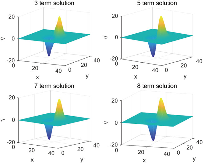
FIGURE 1. Term-wise solutions to linear SWWEs obtained by the MHPM.

The term-wise solutions in $x=22$ and $y=22$ at the same time and depth are presented in Table 3. One may observe that the convergent solution is obtained as the number of terms increasing. It can also be seen from Figure 1 that the images possess a symmetrical property, and the images of non-linear SWWEs in Eq. 2 also have this property. Figures 2–7 show the plane images for the variation in the water surface elevation (WSE) (η) with respect to $x$, when $y$ is fixed at $y=20$. Depending on the symmetry of the images, the same results will be obtained when x has a fixed value.

TABLE 3

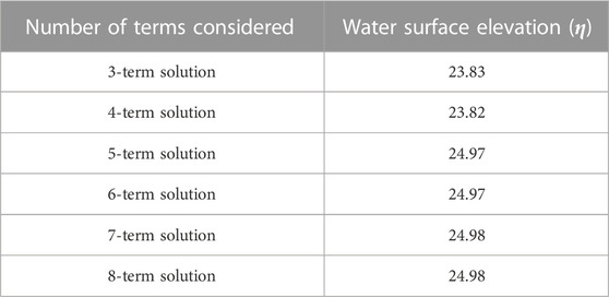
TABLE 3. MHPM at $\mathit{x}\mathit{=}\mathbf{22},\mathit{y}=\mathbf{22}$, and $\mathit{t}=\mathbf{2}\mathit{s},\mathit{h}=.\mathbf{1}$.

FIGURE 2

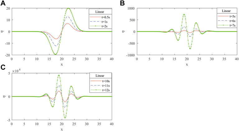
FIGURE 2. WSE of linear SWWEs at $h=.1$ at different time levels.

The water surface elevation (WSE) ($\eta$) of linear SWWEs are depicted at various time levels in Figure 2, at the fixed water depth of $h=.1$. Figure 2A shows the WSE vs. the global coordinate $x$ at three distinct time levels ($t=.5s,1s$, and $2s$), whereas Figures 2B, C represent time levels $t=5s,6s,\mathrm{a}\mathrm{n}\mathrm{d}7s$ and $t=10s,11s,\mathrm{a}\mathrm{n}\mathrm{d}12s$, respectively.

Diagrams in Figure 3 depict changes in the amplitude of linear SWWEs as the basin depth varies from $h=.1$ to $h=.2$ at two different time levels $t=5s$ and $10s$. It can be seen in Table 4 that the WSE increases when the water depth ($h$) increases from .1 to .2 at a fixed time $t=5s$. Similar observations can be found for $t=10s$. Additionally, when time is increased from $t=5s$ to $t=10s$, the WSE increases at a fixed water depth $h=.1$. Similarly, we get comparable results for $h=.2$.

FIGURE 3

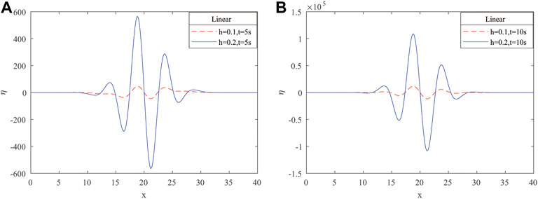
FIGURE 3. WSE of linear SWWEs at $h=.1$ and $h=.2$ at different time levels.

TABLE 4

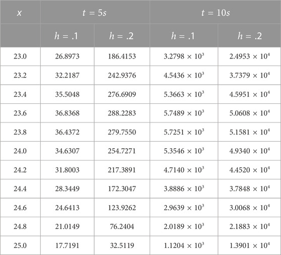
TABLE 4. WSE of linear SWWEs at $5s$ and $10s$ with different $h$ values.

Figure 4 represents the results of WSE of non-linear SWWEs at various time levels with $h=.1$. Also in Figure 4A, the WSE is plotted against the spatial coordinate x at three different time levels $t=.5s,1s$, and $2s$, while Figures 4B, C include results at time levels $t=5s,6s,\mathrm{a}\mathrm{n}\mathrm{d}7s$ and $t=10s,11s,\mathrm{a}\mathrm{n}\mathrm{d}12s$, respectively.

FIGURE 4

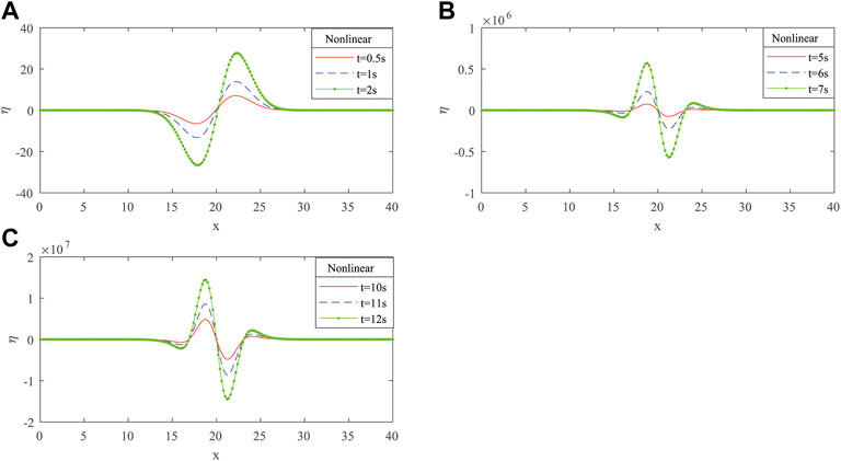
FIGURE 4. WSE of non-linear SWWEs at $h=.1$ at different time levels.

Figure 5 demonstrates changes in non-linear SWWEs as the water depth changes from $h=.1$ to $h=.5$ over two distinct time periods $t=5s$ and $10s$, respectively. Table 5 shows that at a fixed time $t=5s$, the WSE increases when the water depth ($h$) increases from .1 to 0.5. Similar results can be found for $t=10s$. Additionally, at a fixed water depth $h=.1$, the WSE increases when time is increased from $t=5s$ to $t=10s$. We obtain same results when $h=0.5$.

FIGURE 5

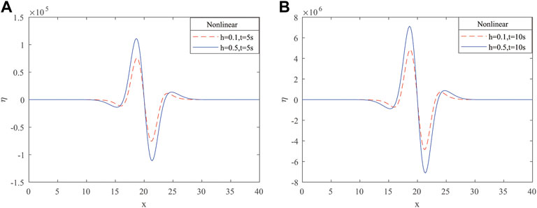
FIGURE 5. WSE of non-linear SWWEs at $h=.1$ and $h=.5$ at different time levels.

TABLE 5

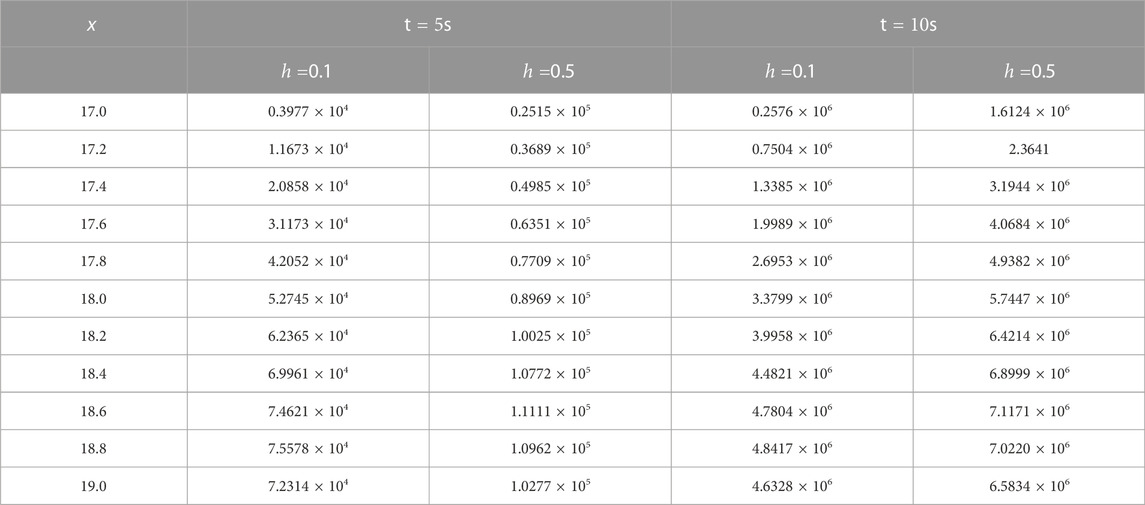
TABLE 5. WSE of nonlinear SWWEs in $5s$ and $10s$ with different h.

Figure 6 shows a comparison graph between the MHPM and HPM for the water surface elevation of the linear SWWEs at the fixed water depth of $h=.1$ at various time levels ($t=2s,5s$). The comparison for the WSE of non-linear SWWEs at fixed $t=2s,5s$ and $h=.1$ by the MHPM and HPM is given in Figure 7, respectively.

FIGURE 6

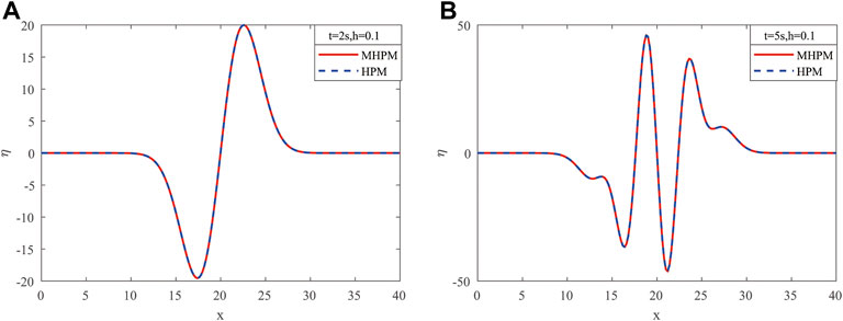
FIGURE 6. WSE of linear SWWEs by the MHPM and HPM at $t=2s$ and $t=5s.$

FIGURE 7

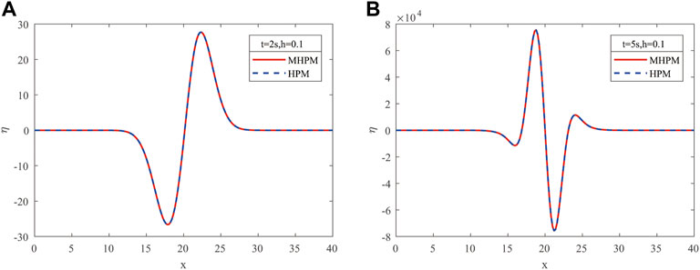
FIGURE 7. WSE of non-linear SWWEs by the MHPM and HPM at $t=2s$ and $t=5s$.

From Figures 2, 4, we may conclude that as time increases, the water surface elevations also increase both in linear and non-linear cases. It can be seen in Figures 3, 5 that the amplitudes of the linear and non-linear shallow water waves increase when the water depth ($h$) increases at a fixed time. The results obtained are consistent with the characteristics of shallow water waves. By comparing Figures 6, 7, the solutions to both linear and non-linear SWWEs obtained by the MHPM are found to be in excellent agreement with the results obtained by the HPM in [6].

5 Conclusion

The main goal of this work is to solve shallow water wave equations using the Mohand transform-based homotopy perturbation method. The variation in the water surface height at different time levels and depths are given in this paper; the results are consistent with the characteristics of shallow water waves. It is proved that this method is a very good tool for solving SWWEs, which can easily be applied in finding out the approximate analytic solutions. The main advantage of this method over the HPM is that it is a powerful and efficient method to determine the analytical solution of the wave equation. In future research, we can also explore the effectiveness of this method in solving other problems, so as to improve the problem-solving efficiency.

Data availability statement

The original contributions presented in the study are included in the article/supplementary material; further inquiries can be directed to the corresponding authors.

Author contributions

Conceptualization, YL, YZ, and JP; methodology, YL, YZ, and JP; software, YL and YZ; validation, YL and JP; writing—original draft preparation, YL, YZ, and JP; writing—review and editing, YL, YZ, and JP; supervision, JP; funding acquisition, JP. All authors have read and agreed to the published version of the manuscript.

Funding

This research was supported by the National Natural Science Foundation of China (Grant No. 10561151), the Basic Science Research Fund in the universities directly under the Inner Mongolia Autonomous Region (Grant No. JY20220003), and the Scientific Research Project of Hetao College (Grant No. HYZQ202122).

Acknowledgments

The authors would like to express their gratitude to the reviewers and editors for their insightful remarks and ideas, which helped them improve the paper’s quality.

Conflict of interest

The authors declare that the research was conducted in the absence of any commercial or financial relationships that could be construed as a potential conflict of interest.

Publisher’s note

All claims expressed in this article are solely those of the authors and do not necessarily represent those of their affiliated organizations, or those of the publisher, the editors, and the reviewers. Any product that may be evaluated in this article, or claim that may be made by its manufacturer, is not guaranteed or endorsed by the publisher.

References

1. Perumandla K, Chakraverty S. Comparison of solutions of linear and non-linear shallow water wave equations using homotopy perturbation method. Int J Numer Methods Heat Fluid flow (2017) 27(9):2015–29. doi:10.1108/HFF-09-2016-0329

CrossRef Full Text | Google Scholar

Liu Y, Shi Y, Yuen D A, Sevre EOD, Yuan X, Xing HL. Comparison of linear and nonlinear shallow wave water equations applied to tsunami waves over the China Sea. Acta Geotechnica (2009) 4(2):129–37. doi:10.1007/s11440-008-0073-0

CrossRef Full Text | Google Scholar

3. Cho YS, Sohn DH, Lee SO. Practical modified scheme of linear shallow-water equations for distant propagation of tsunamis. Ocean Eng (2007) 34(11):1769–77. doi:10.1016/j.oceaneng.2006.08.014

CrossRef Full Text | Google Scholar

4. Tandel P, Patel H, Patel T. Tsunami wave propagation model: A fractional approach. J Ocean Eng Sci (2021) 7:509–20. doi:10.1016/j.joes.2021.10.004

CrossRef Full Text | Google Scholar

5. Wu NJ, Chen C, Tsay TK. Application of weighted-least-square local polynomial approximation to 2D shallow water equation problems. Eng Anal Boundary Elem (2016) 68:124–34. doi:10.1016/j.enganabound.2016.04.010

CrossRef Full Text | Google Scholar

6. Karunakar P, Chakraverty S. 2-D shallow water wave equations with fuzzy parameters. Germany: Springer (2018).

PubMed Abstract | Google Scholar

7. Sahoo M, Chakraverty S. Sawi transform based homotopy perturbation method for solving shallow water wave equations in fuzzy environment. Mathematics (2022) 10:2900. doi:10.3390/math10162900

CrossRef Full Text | Google Scholar

8. Perumandla K, Chakraverty S. Solving shallow water equations with crisp and uncertain initial conditions. Int J Numer Methods Heat Fluid Flow (2018) 28:2801–15. doi:10.1108/hff-09-2017-0351

CrossRef Full Text | Google Scholar

9. Noeiaghdam L, Sidorov DN, Noeiaghdam S. Dynamical control on the homotopy analysis method for solving nonlinear shallow water wave equation. Dynamic Syst Comp Sci Theor Appl (Dysc) (2020) 1847:012010. doi:10.1088/1742-6596/1847/1/012010

CrossRef Full Text | Google Scholar

10. Safari M, Safari M. Analytical solution of two extended model equations for shallow water waves by He's variational iteration method. Am J Comput Math (2011) 1(4):235–9. doi:10.4236/ajcm.2011.14027

CrossRef Full Text | Google Scholar

11. Safari M. Analytical solution of two extended model equations for shallow water waves by adomian's decomposition method. Adv Pure Math (2011) 1(4):238–42. doi:10.4236/apm.2011.14042

CrossRef Full Text | Google Scholar

12. Bekir A, Aksoy E. Exact solutions of extended shallow water wave equations by exp-function method. Int J Numer Methods Heat Fluid Flow (2013) 23(2):305–19. doi:10.1108/09615531311293489

CrossRef Full Text | Google Scholar

13. Mohand M, Mahgoub A. The new integral transform Mohand transform. Appl Math Sci (2017) 12(2):113–20.

Google Scholar

14. Aggarwa S, Sharma N, Chauhan R. Solution of linear volterra integral equations of second kind using Mohand transform. Int J Res Advent Tech (2018) 6(11):3098–102.

Google Scholar

15. Aggarwal S, Vyas A, Sharma SD. Mohand transform for handling convolution type volterra integro-differential equation of first kind. Int J Latest Tech Eng Manag Appl Sci (2020) IX(VII):78–84.

Google Scholar

16. Nadeem M, He JH, Islam A. The homotopy perturbation method for fractional differential equations: Part 1 Mohand transform. Int J Numer Methods Heat Fluid Flow (2021) 31(11):3490–504. doi:10.1108/hff-11-2020-0703

CrossRef Full Text | Google Scholar

17. Khandelwal R, Khandelwal Y. Solution of blasius equation concerning with Mohand transform. Int J Appl Comput Math (2020) 6(5):128. doi:10.1007/s40819-020-00871-w

CrossRef Full Text | Google Scholar

18. Aggarwal S, Chaudhary R. A comparative study of Mohand and Laplace transforms. J Emerging Tech Innovative Res (2019) 6(2):230–40.

Google Scholar

19. Aggarwal S, Sharma N, Chauhan R. Duality relations of kamal transform with Laplace, laplace-carson, Aboodh, Sumudu, Elzaki, Mohand and Sawi transforms. SN Appl Sci (2020) 2(1):135–8. doi:10.1007/s42452-019-1896-z

CrossRef Full Text | Google Scholar

20. Fang JH, Nadeem M, Habib M, Akgül A. Numerical investigation of nonlinear shock wave equations with fractional order in propagating disturbance. Symmetry (2022) 14:1179. doi:10.3390/sym14061179

CrossRef Full Text | Google Scholar

21. Althobaiti S, Dubey RS, Prasad JG. Solution of local fractional generalized fokker-planck equation using local fractional Mohand adomian decomposition method. Fractals (2022) 30(01):2240028. doi:10.1142/s0218348x2240028x

CrossRef Full Text | Google Scholar

22. Shah R, Khan H, Farooq U, Baleanu D, Kumam P, Arif M. A new analytical technique to solve system of fractional-order partial differential equations. IEEE Access (2019) 7:150037–50. doi:10.1109/access.2019.2946946

CrossRef Full Text | Google Scholar

23. He JH. Homotopy perturbation technique. Comp Methods Appl Mech Eng (1999) 178(3-4):257–62. doi:10.1016/s0045-7825(99)00018-3

CrossRef Full Text | Google Scholar

24. Anjum N, He JH. Higher-order homotopy perturbation method for conservative nonlinear oscillators generally and microelectromechanical systems' oscillators particularly. Int J Mod Phys B (2020) 34(32):2050313. doi:10.1142/s0217979220503130

CrossRef Full Text | Google Scholar

25. Yu DN, He JH, Garca AG. Homotopy perturbation method with an auxiliary parameter for nonlinear oscillators. J Low Frequency Noise, Vibration Active Control (2019) 38(3-4):1540–54. doi:10.1177/1461348418811028

CrossRef Full Text | Google Scholar

26. He JH, El-Dib YO. Homotopy perturbation method with three expansions. J Math Chem (2021) 59:1139–50. doi:10.1007/s10910-021-01237-3

CrossRef Full Text | Google Scholar

27. He JH. Application of homotopy perturbation method to nonlinear wave equations. Chaos Solitons and Fractals (2005) 26(3):695–700. doi:10.1016/j.chaos.2005.03.006

CrossRef Full Text | Google Scholar

28. Hemeda AA. Homotopy perturbation method for solving systems of nonlinear coupled equations. Appl Math Sci (2012) 6(96):4787–800.

Google Scholar

29. Madani M, Fathizadeh M, Khan Y, Yildirim A. On the coupling of the homotopy perturbation method and Laplace transformation. Math Comp Model (2011) 53:1937–45. doi:10.1016/j.mcm.2011.01.023

CrossRef Full Text | Google Scholar

30. Mishra HK. A comparative study of variational iteration method and He-Laplace method. Appl Math (2012) 3:1193–201. doi:10.4236/am.2012.310174

CrossRef Full Text | Google Scholar

31. He JH, Moatimid GM, Zekry MH. Forced nonlinear oscillator in a fractal space. Facta Universitatis Series: Mech Eng (2022) 20(1):001–20. doi:10.22190/fume220118004h

CrossRef Full Text | Google Scholar

32. Anjum N, He JH, Ain QT, Tian D. LI-HE’S modified homotopy perturbation method for doubly-clamped electrically actuated microbeams-based microelectromechanical system. Ser Mech Eng (2021) 19(4):601–12. doi:10.22190/fume210112025a

CrossRef Full Text | Google Scholar

33. Li XX, He CH. Homotopy perturbation method coupled with the enhanced perturbation method. J Low Frequency Noise Vibration Active Control (2018) 0(0):1399–403. doi:10.1177/1461348418800554

CrossRef Full Text | Google Scholar

34. He JH, El-Dib YO. The enhanced homotoyp perturbation method for axxial vibration of strings. Facta Universitatis Ser Mech Eng (2021) 19(4):735–50. doi:10.22190/fume210125033h

CrossRef Full Text | Google Scholar

35. He J, El-Dib YO. The reducing rank method to solve third-order Duffing equation with the homotopy perturbation. Numer Methods Partial Differential Equations (2020) 37:1800–8. doi:10.1002/num.22609

CrossRef Full Text | Google Scholar