Direction and distribution sensitivity of sup-DOF interference suppression for GNSS array antenna receiver

Introduction: Distributed wideband jamming (interference) is commonly used in navigation countermeasure. Due to the limited volume of GNSS (Global Navigation Satellite System) array antenna receiver, the number of interferences usually exceeds the number of array elements. At present, the anti-jamming capability and mechanism of Global Navigation Satellite System array antenna against distributed sup-DOF (Degree of Freedom) interference have not been fully studied.

Methods and innovation: To solve this problem, this paper analyzes the characteristics of GNSS System array antenna against sup-Degree of Freedom interference by formula derivation and simulation. Firstly, the definition of sup-Degree of Freedom interference of Global Navigation Satellite System array antenna is proposed from the perspective of spatial anti-jamming; Secondly, the directional characteristics of Global Navigation Satellite System array antenna for sup-Degree of Freedom interference suppression are analyzed.

Results: The results show that the performance of sup-Degree of Freedom interference suppression is sensitive to the direction and distribution of interference. On the one hand, the residual interference power varies from interference direction and distribution, while the minimum value of which is zero and the maximum value is the sum of interference power. On the other hand, the suppression performance of UCA (Uniform Circular Array) and central Uniform Circular Array is periodic along azimuth. If the number of elements on the circumference is M (M ≥ 3), the period of the suppression performance is $\left.4\pi /M/{\left(3+(-1\right)}^{M+1}\right)$.

Discussion: The conclusion of this paper show the upper and lower bounds of sup-Degree of Freedom interference suppression performance and the variation rule in azimuth, which can be used in the fields such as interference deployment, anti-jamming performance evaluation and anti-jamming algorithm development.

1 Introduction

GNSS (Global Navigation Satellite System) provides convenient positioning, navigation and timing services for its application terminals [1]. It has played an important role in transportation, marine fishery, geological disaster monitoring and emergency rescue. However, the GNSS signal power received on ground is weak [2], which is 30 dB lower than the thermal noise of the receiver [3]. The GNSS receiver is vulnerable to unintentional or intentional interference (jamming) under the complex electromagnetic environment, resulting in the receiver performance degradation or failure [4].

Distributed interference is a commonly used interference style in navigation countermeasure [5]. In this case, the number of interferences usually exceeds the number of elements of GNSS antenna array, which might make the receiver unavailable for positioning [6]. On the one hand, it is difficult to completely suppress interferences since the orthogonality between the spatial filter coefficients and the interference steering vectors no longer exist [7, 8]. On the other hand, most GNSS array antennas have only 4–7 elements [9, 10]. Due to limited space of navigation facilities, half wavelength of L-band GNSS signal and low cost of interference equipment, it is easier to increase the number of interferences than the number of array elements [11, 12].

There is a lack of definition of sup-degree-of-freedom interference in GNSS anti-jamming research. In array signal processing, it is generally considered that the DOF (Degree of Freedom) of an array with N elements is N-1. In the field such as sparse array [13], virtual array [14], polarized array antenna [15] and synthetic aperture [16], there is only the concept of “interference exceeds array DOF” without clear definition; In the field of DOA (Direction of Arrival) estimation, direction estimation ambiguity is defined and classified [17, 18], which provides reference for the study of interference direction against array DOF; Some researchers propose that N-element GNSS antenna array receiver can at most suppress N-1 interference [19], but this statement is not accurate considering the preconditions for the conclusion are not clearly explained, and the signal types and parameters are not limited; At the same time, most beamforming algorithms and DOA estimation algorithms focus on the precondition that the number of interference is less than N [20, 21]. In order to further study the anti-jamming characteristics of array antenna while the number of interferences is equal or larger than N, a clear and simple definition of sup-degree-of-freedom interference is needed to specify the background. It would be better if the definition focuses on the array anti-jamming module rather than considering the positioning performance of GNSS receivers. Otherwise, parameters related to signal and data processing should be further introduced [22], such as receiver acquisition and tracking threshold and DOP (Dilution of Precision) constrains, which makes the definition complicated.

To solve the above problems, from the perspective of spatial anti-jamming, this paper first analyzes the precondition that N-element array can suppress at most N-1 interferences, and proposes the definition of sup-DOF interference; Secondly, according to theoretical analysis and simulation, the paper proposes that the suppression performance of array antenna is sensitive to direction and distribution of sup-DOF interference. The structure of the paper is as follows: In the second section, the model of array signal reception and anti-jamming is established; In the third section, the definition of sup-DOF interference is proposed and is explained by numerical calculation; In the fourth section, based on theoretical analysis and numerical calculation, it is proposed that the suppression performance has directional sensitivity, distribution sensitivity, as well as azimuthal periodicity; In the fifth section, the conclusion in the fourth section is verified by simulation; The structure block diagram of the article is shown in Figure 1, in which the orange part is the innovation of this article.

FIGURE 1

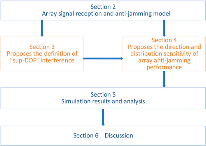
FIGURE 1. Article structure block diagram.

For the convenience of reading, the commonly used symbols in this paper are shown in Table 1. In the text, symbols in italics represent variables, and non-italics in bold represent vectors or matrices.

TABLE 1

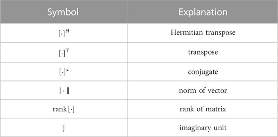
TABLE 1. Common symbols in this article.

2 Signal reception and anti-jamming model of antenna array

Suppose that the navigation signal and interference signal are received by an N-element array antenna. Denote navigation signal, signal power and steering vector as $s\left(t\right)$, $p_s$, and ${\mathbf{a}}_{\mathbf{s}}$ respectively. Denote the interference, power and steering vector as $j\left(t\right)$, $p_j$, and ${\mathbf{a}}_{\mathbf{j}}$ respectively. Denote the noise power as $p_n$, while t represents time. The steering vector is N × 1 dimensional column vector. Let the number of navigation signals and interference be I and K respectively, the received signal of N-element array is

$\mathbf{x}\left(t\right)={\displaystyle \sum }_{i=1}^I{p}_{s_i}{s}_i\left(t\right){\mathbf{a}}_{{\mathbf{s}}_{\mathbf{i}}}+{\displaystyle \sum }_{k=1}^K{p}_{j_k}{j}_k\left(t\right){\mathbf{a}}_{{\mathbf{j}}_{\mathbf{k}}}+\sqrt{p_n}{\mathbf{n}}_{\mathbf{N}}\left(t\right)(1)$

where i represents the ith navigation signal, k represents the kth interference signal, and ${\mathbf{n}}_{\mathbf{N}}\left(\mathbf{t}\right)$ represents the thermal noise of the N-dimensional array. The steering vector is composed by the signal phase difference between each array element and the reference element. In order to simplify the analysis, the non-ideal factors that cause the steering vector mismatch is ignord, and the narrowband signal model is adopted. The steering vector has the following form, where ${\tau }_1,{\tau }_2,\cdots {\tau }_{N-1}$ is the time delay between the received signal of each array element and the reference element, and $f_c$ is the carrier frequency.

$\mathbf{a}={\left[\begin{array}{cccc}1& \exp \left[\mathrm{j}2\pi f_c{\tau }_1\right]& \cdots & \exp \left[\mathrm{j}2\pi f_c{\tau }_{N-1}\right]\end{array}\right]}^{\mathrm{T}}(2)$

Denote the normalized spatial filter coefficient as $\overline{\mathbf{w}}$.it is an N × 1 dimensional column vector with the modulus of 1.

$\overline{\mathbf{w}}={\left[\begin{array}{cccc}{w}_1& w_2& \cdots & w_N\end{array}\right]}^T(3)$

$‖\overline{\mathbf{w}}‖=1(4)$

Then the output signal of spatial anti-jamming processing is

$y\left(t\right)={\overline{\mathbf{w}}}^{\mathrm{H}}\mathbf{x}\left(t\right)(5)$

If interference signals are independent of each other, the covariance matrix of interference signals is

${\mathbf{R}}_{\mathbf{j}\mathbf{j}}={\displaystyle \sum }_{k=1}^K{p}_{j_k}{\mathbf{a}}_{{\mathbf{j}}_{\mathbf{k}}}{\mathbf{a}}_{{\mathbf{j}}_{\mathbf{k}}}^{\mathrm{H}}(6)$

3 Definition of sup-DOF interference and numerical analysis

In array signal processing, it is generally considered that the DOF of an N-element array is N-1. However, the statement that N-element array can suppress at most N-1 interferences is not accurate. In this section, from the perspective of spatial anti-jamming, the preconditions for the above statement are analyzed, and the definition of sup-DOF interference is proposed.

3.1 Definition of sup-DOF interference

According to Eqs 1, 5, the residual interference signal is

$y_j\left(t\right)={\overline{\mathbf{w}}}^{\mathrm{H}}{\displaystyle \sum }_k{j}_k\left(t\right){\mathbf{a}}_{{\mathbf{j}}_{\mathbf{k}}}(7)$

There are two ways to interpret principle of spatial interference suppression. One is to figure out $\overline{\mathbf{w}}$ satisfies $\overline{\mathbf{w}}\ne \mathbf{0}$ and the following equation set

$\left\{\begin{array}{c}{\overline{\mathbf{w}}}^{\mathrm{H}}{\mathbf{a}}_{{\mathbf{j}}_{\mathbf{1}}}{j}_1\left(t\right)=0\\ {\overline{\mathbf{w}}}^{\mathrm{H}}{\mathbf{a}}_{{\mathbf{j}}_{\mathbf{2}}}{j}_2\left(t\right)=0\\ ⋮\\ {\overline{\mathbf{w}}}^{\mathrm{H}}{\mathbf{a}}_{{\mathbf{j}}_{\mathbf{K}}}{j}_K\left(t\right)=0\end{array}\right.(8)$

The constrains make sure that the antenna gain of direction described by ${\mathbf{a}}_{{\mathbf{j}}_{\mathbf{k}}}$ is 0, thus suppress the interference coming from this direction. The other way is to solve $\overline{\mathbf{w}}$ that makes the residual interference power zero:

$p_{jres}=E\left\{\left({\displaystyle \sum }_{k=1}^K{\overline{\mathbf{w}}}^{\mathrm{H}}{\mathbf{a}}_{{\mathbf{j}}_{\mathbf{k}}}{j}_k(t))\cdot \right({\displaystyle \sum }_{k=1}^K{\overline{\mathbf{w}}}^{\mathrm{H}}{\mathbf{a}}_{{\mathbf{j}}_{\mathbf{k}}}{j}_k\left(t\right){)}^{*}\right\}=0(9)$

where $p_{jres}$ is the residual interference power.

Denote the interference steering vector matrix as

${\mathbf{A}}_{\mathbf{j}}=\left[\begin{array}{cccc}{\mathbf{a}}_{{\mathbf{j}}_{\mathbf{1}}}& {\mathbf{a}}_{{\mathbf{j}}_{\mathbf{2}}}& \cdots & {\mathbf{a}}_{{\mathbf{j}}_{\mathbf{K}}}\end{array}\right](10)$

According to Eq. 6, the covariance matrix of the interference signal is non-negative. As a result, Eq. 8 is equivalent to the following form:

${\overline{\mathbf{w}}}^{\mathrm{H}}{\mathbf{A}}_{\mathbf{j}}={\mathbf{0}}_{\mathbf{r}}(11)$

where ${\mathbf{0}}_{\mathbf{r}}$ is a row vector, ${\mathbf{A}}_{\mathbf{j}}$ is an and matrix of dimension N×K. Denote the rank of ${\mathbf{A}}_{\mathbf{j}}$ as $rank\left({\mathbf{A}}_{\mathbf{j}}\right)$, the maximum value of $rank\left({\mathbf{A}}_{\mathbf{j}}\right)$ is N. Analyze the solution set of Eq. 8. If $rank\left({\mathbf{A}}_{\mathbf{j}}\right)$ ≤ N-1, $\overline{\mathbf{w}}$ satisfies Eq. 8 and $\overline{\mathbf{w}}\ne \mathbf{0}$, thus the interferences can be completely suppressed. If $rank\left({\mathbf{A}}_{\mathbf{j}}\right)$ = N, Eq. 8 is satisfied only if $\overline{\mathbf{w}}=\mathbf{0}$, thus the navigation signal cannot be retained while suppressing interference, and anti-interference processing becomes invalid. It can be seen that for mutually independent interferences, the anti-jamming ability of the N-element array antenna depends not only on the number of interferences, but also on the spatial correlation of the interference signal steering vector. The precondition for the N-element array to suppress at most N-1 interference is that the steering vectors of the interference signal are linearly uncorrelated. The precondition for N-element array to suppress more than N-1 interferences is that the rank of the interference steering vector matrix is not greater than N-1.

Under the condition that the interferences are independent of each other, the definition of array sup-DOF interference is proposed according to spatial anti-jamming principle.

Definition 1: Assume interferences are independent of each other, and their steering vectors can be represented by a finite number of column vectors. When the number of interferences simultaneously received by the antenna array is greater than or equal to the number of array elements N, and at least N steering vectors are linearly uncorrelated, it is defined that the number of interferences surpass the array degree of freedom.

This definition can be described as follows:

$\left\{\begin{array}{c}rank\left({\mathbf{A}}_{\mathbf{j}}\right)<Ninterferencesdonotsurpassthearraydegreeoffreedom\\ rank\left({\mathbf{A}}_{\mathbf{j}}\right)=Ninterferencessurpassthearraydegreeoffreedom\end{array}\right.(12)$

The above definition is only applicable to the case where interference signals are independent of each other. If the interference signal has correlation, or the steering vector of the signal cannot be represented by a limited number of column vectors, the interference suppression principle can be analyzed through the residual interference power of anti-jamming processing.

According to Eq. 7, the residual interference power is

$p_{jres}=E\left\{y_j\left(t\right)y_j^{*}\left(t\right)\right\}(13)$

The above equation can be written as

$p_{jres}={\overline{\mathbf{w}}}^{\mathrm{H}}{\mathbf{R}}_{\mathbf{j}\mathbf{j}}\overline{\mathbf{w}}(14)$

For GNSS array antenna receiver, the goal of anti-jamming process is to make the residual interference power zero, while retaining the navigation signal as much as possible. That is to say, the solution $\overline{\mathbf{w}}$ satisfies $\overline{\mathbf{w}}\ne \mathbf{0}$ while

$p_{jres}={\overline{\mathbf{w}}}^{\mathrm{H}}{\mathbf{R}}_{\mathbf{j}\mathbf{j}}\overline{\mathbf{w}}=0(15)$

According to Rayleigh entropy theorem, the value range of interference residual power is

${\lambda }_{\min }\le p_{jres}\le {\lambda }_{\max }(16)$

where ${\lambda }_{\min }$ and ${\lambda }_{\max }$ is the minimum and maximum eigenvalues of ${\mathbf{R}}_{\mathbf{j}\mathbf{j}}$. The equal signs are taken when $\overline{\mathbf{w}}$ equals to the corresponding eigenvector. In this case, the residual interference power of the anti-jamming process is optimized.

If the minimum eigenvalue of ${\mathbf{R}}_{\mathbf{j}\mathbf{j}}$ is zero, the residual power is 0, and the interference signal is completely suppressed, which means that ${\mathbf{R}}_{\mathbf{j}\mathbf{j}}$ is not a full-rank matrix; If the minimum eigenvalue of ${\mathbf{R}}_{\mathbf{j}\mathbf{j}}$ is not zero, the interference signal cannot be completely suppressed, at this moment ${\mathbf{R}}_{\mathbf{j}\mathbf{j}}$ is a full-rank matrix.

Thus, the sup-DOF interference can be defined by the rank of the interference covariance matrix:

Definition 2: Assume the number of interferences received by the array antenna simultaneously is K (K ≥ 1). If the rank of the covariance matrix of the received interference equals to the number of antenna elements N, the interferences surpass the array degree of freedom. The above interferences are collectively referred to as array sup-degree of freedom interference, or sup-DOF interference for short.

Denote the rank of the interference covariance matrix as $rank\left({\mathbf{R}}_{\mathbf{j}\mathbf{j}}\right)$. This definition can be described as

$\left\{\begin{array}{c}rank\left({\mathbf{R}}_{\mathbf{j}\mathbf{j}}\right)<Ninterferencesdonotsurpassthearraydegreeoffreedom\\ rank\left({\mathbf{R}}_{\mathbf{j}\mathbf{j}}\right)=Ninterferencessurpassthearraydegreeoffreedom\end{array}\right.(17)$

According to Formula. 17, $rank\left({\mathbf{R}}_{\mathbf{j}\mathbf{j}}\right)$ is only related to the second-order statistical characteristics of the received array interference. The scope of application of this definition has no limit on the signal correlation and spatial correlation of the interference signals.

Based on the above analysis, the following conclusion can be drawn:

Conclusion 1: If the number of interferences is greater than or equal to the number of array elements (K ≥ N), the interference may not surpass the array degree of freedom. The existence of a specific direction allows the antenna array to completely suppress K interferences.

The specific incident directions in conclusion 1 can be divided into two categories. The first category is that the incident directions of interference are different, while their steering vectors are equal or conjugate; The second category is that the K steering vectors corresponding to different incident angles are correlated with each other and can be represented by N-1 vectors. Among them, it is difficult to find the incident direction of the second category by enumerating. Finding the incident direction of the second category has become an open problem in the field of differential geometry, which will not be further researched in this paper.

3.2 Numerical calculation and analysis

Taking the central UCA (Uniform Circular Array) of four elements as an example, the typical interference incidence direction is taken to further explain conclusion 1. The coordinates of array element are given in Eq. 18. Assume that the power of interferences in Figure 2 is 1, and the interference signals are independent of each other. In Figure 2A, the incident direction of interference 1 is $\left[{\theta }_{j_1},{\phi }_{j_1}\right]$. Interference 1 and interference 2 are symmetrical about the xOy plane, interference 1 and interference 3 are opposite in the incident direction, interference 1 and interference 4 have the same incident elevation angle, and the azimuth difference is π. The incident directions of interference 2, 3, and 4 are $\left[-{\theta }_{j_1},{\phi }_{j_1}\right]$, $\left[-{\theta }_{j_1},-{\phi }_{j_1}\right]$ and $\left[{\theta }_{j_1},{\phi }_{j_1}+\pi \right]$ respectively.

FIGURE 2

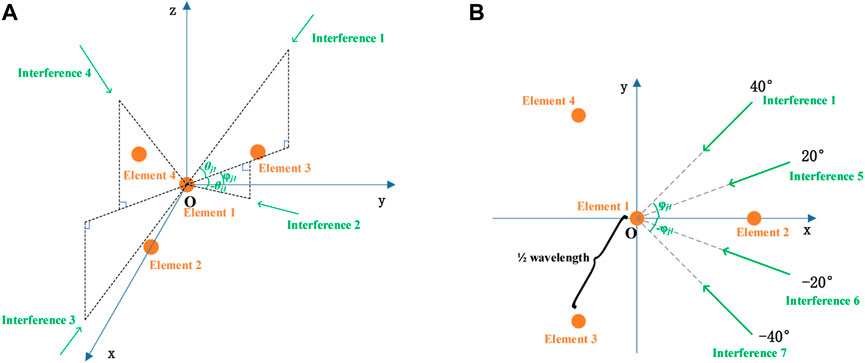
FIGURE 2. The position of the central UCA with four elements in the Oxyz coordinate system. (A) Three-dimensional figure; (B) xOy Planar 2D figure.

In the Oxyz coordinate system, the array element coordinate matrix is as follows. The first, second and third columns of the matrix are respectively the x, y, and z coordinates of the array element, and ${\lambda }_c$ is the signal carrier wavelength.

${\mathbf{P}}_{\mathbf{e}\mathbf{l}\mathbf{e}}=\left[\begin{array}{ccc}0& 0& 0\\ \frac{1}{2}{\lambda }_c& 0& 0\\ -\frac{1}{2}{\lambda }_c& \frac{\sqrt{3}}{2}{\lambda }_c& 0\\ -\frac{1}{2}{\lambda }_c& -\frac{\sqrt{3}}{2}{\lambda }_c& 0\end{array}\right](18)$

The interference steering vector is

${\mathbf{a}}_{{\mathbf{j}}_{\mathbf{k}}}=\exp \left[\mathrm{j}2\pi f_c\frac{{\mathbf{P}}_{\mathbf{e}\mathbf{l}\mathbf{e}}{\mathbf{r}}_{{\mathbf{j}}_{\mathbf{k}}}}{c}\right](19)$

where $c$ is the speed of light, ${\mathrm{r}}_{{\mathrm{j}}_{\mathrm{k}}}$ is the unit direction vector, and $f_c$ is the carrier frequency.

${\mathbf{r}}_{{\mathbf{j}}_{\mathbf{k}}}=\left[\begin{array}{c}\cos {\theta }_{j_k}\cos {\phi }_{j_k}\\ \cos {\theta }_{j_k}\sin {\phi }_{j_k}\\ \sin {\theta }_{j_k}\end{array}\right](20)$

Simplify the steering vector expression, it can be written as

${\mathbf{a}}_{{\mathbf{j}}_{\mathbf{k}}}=\exp \left\{\mathrm{j}\pi \cos {\theta }_{j_k}\left[\begin{array}{c}0\\ \cos {\phi }_{j_k}\\ \sin \left({\phi }_{j_k}-\frac{\pi }{6}\right)\\ -\sin \left({\phi }_{j_k}+\frac{\pi }{6}\right)\end{array}\right]\right\}(21)$

The steering vectors of interference 1–4 is

${\mathbf{a}}_{{\mathbf{j}}_{\mathbf{1}}}={\mathbf{a}}_{{\mathbf{j}}_2}=\left[\begin{array}{c}1\\ \exp \left[\mathrm{j}\pi \cos {\theta }_{j_1}\cos {\phi }_{j_1}\right]\\ \exp \left[\mathrm{j}\pi \cos {\theta }_{j_1}\sin \left({\phi }_{j_1}-\frac{\pi }{6}\right)\right]\\ \exp \left[-\mathrm{j}\pi \cos {\theta }_{j_1}\sin \left({\phi }_{j_1}+\frac{\pi }{6}\right)\right]\end{array}\right],{\mathbf{a}}_{{\mathbf{j}}_{\mathbf{3}}}={\mathbf{a}}_{{\mathbf{j}}_{\mathbf{4}}}=\left[\begin{array}{c}1\\ \exp \left[-\mathrm{j}\pi \cos {\theta }_{j_1}\cos {\phi }_{j_1}\right]\\ \exp \left[-\mathrm{j}\pi \cos {\theta }_{j_1}\sin \left({\phi }_{j_1}-\frac{\pi }{6}\right)\right]\\ \exp \left[\mathrm{j}\pi \cos {\theta }_{j_1}\sin \left({\phi }_{j_1}+\frac{\pi }{6}\right)\right]\end{array}\right](22)$

It can be seen that the steering vectors of interference 1 and 2 are conjugate with interference 3 and 4. According to Eq. 6, the covariance matrix of each interference can be obtained as follows

${\mathbf{R}}_{{\mathbf{j}}_{\mathbf{1}}}={\mathbf{R}}_{{\mathbf{j}}_{\mathbf{2}}}={\mathbf{R}}_{{\mathbf{j}}_{\mathbf{3}}}={\mathbf{R}}_{{\mathbf{j}}_{\mathbf{4}}}(23)$

Denote the steering vector matrix and covariance matrix of the above four interferences as ${\mathbf{A}}_{\mathbf{j}\_1}$ and ${\mathbf{R}}_{\mathbf{j}\mathbf{j}\_1}$ respectively. Considering the sup-DOF interference definition 1 and definition 2, it can be obtained that

$rank\left({\mathbf{A}}_{\mathbf{j}\_1}\right)=1(24)$

$rank\left({\mathbf{R}}_{\mathbf{j}\mathbf{j}\_1}\right)=1(25)$

Therefore, the above four interferences are equivalent to one interference. Interference 1–4 belong to the incident direction of first category interference mentioned at the end of Section 3.1.

Denote the incident directions of four interference in Figure 2B are $\left[{\theta }_{j_1},{\phi }_{j_1}\right]$, $\left[{\theta }_{j_5},{\phi }_{j_5}\right]$, $\left[{\theta }_{j_6},{\phi }_{j_6}\right]$ and $\left[{\theta }_{j_7},{\phi }_{j_7}\right]$ respectively. The four incident directions have the following relationship:

${\theta }_{j_1}={\theta }_{j_5}={\theta }_{j_6}={\theta }_{j_7}(26)$

${\phi }_{j_1}=-{\phi }_{j_7},{\phi }_{j_5}=-{\phi }_{j_6}(27)$

Denote the steering vector matrix and covariance matrix of the above four interferences as ${\mathbf{A}}_{\mathbf{j}\_2}$ and ${\mathbf{R}}_{\mathbf{j}\mathbf{j}\_2}$ respectively,

${\mathbf{A}}_{\mathbf{j}\_2}=\left[\begin{array}{cccc}{\mathbf{a}}_{{\mathbf{j}}_1}& {\mathbf{a}}_{{\mathbf{j}}_5}& {\mathbf{a}}_{{\mathbf{j}}_6}& {\mathbf{a}}_{{\mathbf{j}}_7}\end{array}\right](28)$

${\mathbf{R}}_{\mathbf{j}\mathbf{j}\_2}={\displaystyle \sum }_{\mathbf{k}=\mathbf{1,5,6,7}}{\mathbf{a}}_{{\mathbf{j}}_{\mathbf{k}}}{\mathbf{a}}_{{\mathbf{j}}_{\mathbf{k}}}^{\mathbf{H}}(29)$

It can be simplified that

${\mathbf{R}}_{\mathbf{j}\mathbf{j}\_2}=\left[\begin{array}{cccc}1& 0& 0& r_{14}\\ 0& 1& 0& r_{24}\\ 0& 0& 1& -1\\ 0& 0& 0& 0\end{array}\right](30)$

Among which

$\begin{array}{l}{r}_{14}={\mathrm{e}}^{\mathrm{j}\pi \cos {\theta }_{j_1}\left[3\cos {\phi }_{j_5}+\sqrt{3}\sin {\phi }_{j_5}\right]}\times \\ \frac{{-1+\mathrm{e}}^{\mathrm{j}\pi \cos {\theta }_{j_1}\left(3\cos {\phi }_{j1}-3\cos {\phi }_{j_5}+\sqrt{3}\sin {\phi }_{j_1}-\sqrt{3}\sin {\phi }_{j_5}\right)}{-\mathrm{e}}^{-2\sqrt{3}\mathrm{j}\pi \cos {\theta }_{j_1}\sin {\phi }_{j_5}}+{\mathrm{e}}^{\mathrm{j}\pi \cos {\theta }_{j_1}\left(3\cos {\phi }_{j1}-3\cos {\phi }_{j_5}-\sqrt{3}\sin {\phi }_{j_1}-\sqrt{3}\sin {\phi }_{j_5}\right)}}{{\mathrm{e}}^{2\mathrm{j}\pi \cos {\phi }_{j_1}\cos {\theta }_{j_1}}{-\mathrm{e}}^{2\mathrm{j}\pi \cos {\phi }_{j_5}\cos {\theta }_{j_1}}}\end{array}(31)$

$r_{24}=\frac{{\mathrm{e}}^{2\mathrm{j}\pi \cos {\theta }_{j_1}\left[\cos {\phi }_{j_1}+\cos {\phi }_{j_5}\right]}\times \left[{\mathrm{e}}^{-2\mathrm{j}\pi \cos {\theta }_{j_1}\sin \left({\phi }_{j_1}-\frac{\pi }{6}\right)}{-\mathrm{e}}^{-2\mathrm{j}\pi \cos {\theta }_{j_1}\sin \left({\phi }_{j_5}-\frac{\pi }{6}\right)}+{\mathrm{e}}^{2\mathrm{j}\pi \cos {\theta }_{j_1}\sin \left({\phi }_{j_1}+\frac{\pi }{6}\right)}{-\mathrm{e}}^{2\mathrm{j}\pi \cos {\theta }_{j_1}\sin \left({\phi }_{j_5}+\frac{\pi }{6}\right)}\right]}{-{\mathrm{e}}^{2\mathrm{j}\pi \cos {\phi }_{j_1}\cos {\theta }_{j_1}}+{\mathrm{e}}^{2\mathrm{j}\pi \cos {\phi }_{j_5}\cos {\theta }_{j_1}}}(32)$

It can be seen that the rank of the covariance matrix is 3, and the rank of the guidance vector matrix is 3.

$rank\left({\mathbf{A}}_{\mathbf{j}\_2}\right)=3(33)$

$rank\left({\mathbf{R}}_{\mathbf{j}\mathbf{j}\_2}\right)=3(34)$

Interference 1, 5, 6, and interference 7 exist in the subspace of dimension-3, so they are equivalent to three interferences. They belong to the incident direction of the second category interference mentioned at the end of Section 3.1.

4 Direction and distribution sensitivity of sup-DOF interference suppression

If the number of interferences is greater than or equal to the number of array elements (K ≥ N), the spatial anti-jamming algorithm may not completely suppress them. According to Eq. 16, the residual interference power obtained by optimal spatial filter is the minimum eigenvalue of the interference covariance matrix, so the minimum eigenvalue of the interference signal covariance matrix can be used to characterize the anti-jamming performance. Denote the minimum eigenvalue as the optimal residual interference power, this section will specifically analyze the interference suppression performance on the condition of K ≥ N.

4.1 Influence of interference direction and distribution of super-DOF interference on residual interference power

According to the typical interference deployment scenarios in navigation countermeasure, the sup-DOF interferences are usually gathered in certain space angles while their exact locations are uncertain [23]. To study the rules of anti-sup-DOF-jamming performance, it is simpler to depict a cluster of jammers by their DOA boundaries rather than concentrate on specific jammer configurations. As a result, the interference deployment is described in the following parameters. Suppose the interference number is K, the incident angle in elevation is ${\theta }_{j_1},{\theta }_{j_2},\cdots {\theta }_{j_K}$, the azimuth angle is ${\phi }_{j_1},{\phi }_{j_2},\cdots {\phi }_{j_k}$, and the power is $p_{j_1}=p_{j_2}=\cdots =p_{j_K}$. In order to describe the positions of the K interferences, the central incident direction of the interferences is defined as $\left[{\theta }_{j_0},{\phi }_{j_0}\right]$, and the interference distribution is simplified as $\left[\Delta {\Theta }_j,\Delta {\vartheta }_j\right]$. Their expressions are as follows.

$\left\{\begin{array}{l}{\theta }_{j_0}=\frac{{\displaystyle \sum }_{k=1}^K{\theta }_{j_k}}{K}\\ {\phi }_{j_0}=\frac{{\displaystyle \sum }_{k=1}^K{\phi }_{j_k}}{K}\end{array}\right.(35)$

$\left\{\begin{array}{l}\Delta \Theta =\max \left\{\left|{\theta }_{j_i}-{\theta }_{j_l}\left|\right|i,l\in \left[1,K\right],i\ne j\right.\right\}\\ \Delta \vartheta =\max \left\{\left|{\phi }_{j_i}-{\phi }_{j_l}\left|\right|i,l\in \left[1,K\right],i\ne j\right.\right\}\end{array}\right.(36)$

See Figure 3 for the schematic diagram of the central incident direction and distribution.

FIGURE 3

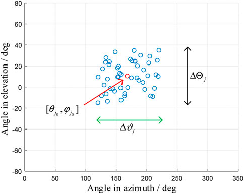
FIGURE 3. Schematic diagram of central incident direction and interference distribution.

In order to simplify the analysis of the central incident direction and distribution, the interference signals are assumed to be independent and the intersection angle of adjacent interferences are equal. A two-element antenna is taken as an example for analysis.

The positions of the two elements are shown in Figure 4. Its coordinates are as follows, where ${\lambda }_c$ is the signal carrier wavelength.

${\mathbf{P}}_{\mathbf{2}\mathbf{e}\mathbf{l}\mathbf{e}}=\left[\begin{array}{l}\begin{array}{ccc}{x}_1& y_1& z_1\end{array}\\ \begin{array}{ccc}{x}_2& y_2& z_2\end{array}\end{array}\right]=\left[\begin{array}{l}\begin{array}{ccc}0& 0& 0\end{array}\\ \begin{array}{ccc}0& 0& \frac{1}{2}{\lambda }_c\end{array}\end{array}\right](37)$

FIGURE 4

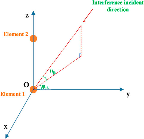
FIGURE 4. Position of two-element array in Oxyz coordinate system.

The steering vector of the kth interference is

${\mathbf{a}}_{{\mathbf{j}}_{\mathbf{k}}}=\exp \left\{\mathrm{j}\pi \left[\begin{array}{c}0\\ \sin {\theta }_{j_k}\end{array}\right]\right\}(38)$

The characteristic polynomial of the interference covariance matrix is a one-variable quadratic equation about the eigenvalue $\lambda$:

$f\left(\lambda \right)=\left|\lambda \mathbf{I}-{\mathbf{R}}_{\mathbf{j}\mathbf{j}}\right|={\lambda }^2-\left({\mathbf{M}}_{\mathbf{11}}+{\mathbf{M}}_{\mathbf{22}}\right)\cdot \lambda +\left|{\mathbf{R}}_{\mathbf{j}\mathbf{j}}\right|(39)$

Wherein, ${\mathbf{M}}_{\mathbf{11}}$ and ${\mathbf{M}}_{\mathbf{22}}$ are the algebraic cofactors of two diagonal elements respectively, $\left|\cdot \right|$ representing the determinant of the matrix.

Take two independent interferences as an example. Set the interference power as $p_{j_1}$ and $p_{j_2}$ respectively. The interference central direction and distribution are set as follows.

${\theta }_{j_0}=\frac{{\theta }_{j_1}+{\theta }_{j_2}}{2}(40)$

$\Delta {\mathrm{\Theta }}_j=‖{\theta }_{j_2}-{\theta }_{j_1}‖(41)$

Combine Eq. 6 and Eq. 39, let $f\left(\lambda \right)=0$, then the optimal residual interference power is obtained:

$p_{jres}\left({\theta }_{j_0},\Delta {\mathrm{\Theta }}_j\right)=\left(p_{j_1}+p_{j_2}\right)-\sqrt{\left(p_{j_1}+p_{j_2}{)}^2-2p_{j_1}{p}_{j_2}(1-\cos (\pi \sin ({\theta }_{j_0}-\frac{\Delta {\Theta }_j}{2})-\pi \sin ({\theta }_{j_0}+\frac{\Delta {\Theta }_j}{2})\right)}(42)$

The partial derivative of the above equation is obtained from ${\theta }_{j_0}$ and $\Delta {\Theta }_j$:

$\left\{\begin{array}{l}\frac{\partial p_{jres}\left({\theta }_{j_0},\Delta {\mathrm{\Theta }}_j\right)}{\partial \Delta {\mathrm{\Theta }}_j}=\frac{-p_{j_1}{p}_{j_2}\pi \sin \left[\pi \sin \left({\theta }_{j_0}-\frac{\Delta {\mathrm{\Theta }}_j}{2}\right)-\pi \sin \left({\theta }_{j_0}+\frac{\Delta {\mathrm{\Theta }}_j}{2}\right)\right]\cdot \left[\cos \left({\theta }_{j_0}-\frac{\Delta {\mathrm{\Theta }}_j}{2}\right)+\cos \left({\theta }_{j_0}+\frac{\Delta {\mathrm{\Theta }}_j}{2}\right)\right]}{2\sqrt{\left(p_{j_1}+p_{j_2}{)}^2-2p_{j_1}{p}_{j_2}(1-\cos (\pi \sin ({\theta }_{j_0}-\frac{\Delta {\mathrm{\Theta }}_j}{2})-\pi \sin ({\theta }_{j_0}+\frac{\Delta {\mathrm{\Theta }}_j}{2})\right)}}\\ \frac{\partial p_{jres}\left({\theta }_{j_0},\Delta {\mathrm{\Theta }}_j\right)}{\partial {\theta }_{j_0}}=\frac{p_{j_1}{p}_{j_2}\pi \sin \left[\pi \sin \left({\theta }_{j_0}-\frac{\Delta {\mathrm{\Theta }}_j}{2}\right)-\pi \sin \left({\theta }_{j_0}+\frac{\Delta {\mathrm{\Theta }}_j}{2}\right)\right]\cdot \left[\cos \left({\theta }_{j_0}-\frac{\Delta {\mathrm{\Theta }}_j}{2}\right)-\cos \left({\theta }_{j_0}+\frac{\Delta {\mathrm{\Theta }}_j}{2}\right)\right]}{\sqrt{\left(p_{j_1}+p_{j_2}{)}^2-2p_{j_1}{p}_{j_2}(1-\cos (\pi \sin ({\theta }_{j_0}-\frac{\Delta {\mathrm{\Theta }}_j}{2})-\pi \sin ({\theta }_{j_0}+\frac{\Delta {\mathrm{\Theta }}_j}{2})\right)}}\end{array}\right.(43)$

It can be seen from the observation that it is difficult to simplify $p_{jres}\left({\theta }_{j_0},\Delta {\Theta }_j\right)$ to the multiplication of two one-variable functions. The central incident direction is closely coupled with the interference distribution.

If $\Delta {\Theta }_j\ne 0$, let

$\frac{\partial p_{jres}\left({\theta }_{j_0},\Delta {\mathrm{\Theta }}_j\right)}{\partial {\theta }_{j_0}}=0(44)$

The central interference incident direction that minimizes the optimal residual interference power can be solved

${\theta }_{j_0}=\frac{\pi }{2}+\pi l,l=0,\pm 1,\pm 2,\cdots (45)$

Combine Eq. 45 with Eq. 42, it can be obtained that

$p_{jres}\left({\theta }_{j_0},\Delta {\mathrm{\Theta }}_j\right)=0(46)$

Extending to K interferences (K ≥ 2), the optimal residual interference power is

$p_{jres}={\displaystyle \sum }_{k=1}^K{p}_{j_k}-\sqrt{{\left({\displaystyle \sum }_{k=1}^K{p}_{j_k}\right)}^2-2{\displaystyle \sum }_{\underset{u\ne v}{u=1,v=1}}^K{p}_{j_u}{p}_{j_v}\left(1-\cos \left(\pi \sin {\theta }_{j_u}-\pi \sin {\theta }_{j_v}\right)\right)}(47)$

According to the above formula, if $\cos \left(\pi \sin {\theta }_{j_u}-\pi \sin {\theta }_{j_v}\right)=1$, the optimal residual interference power reaches the minimum value $p_{jres,\min }=0$; If $\cos \left(\pi \sin {\theta }_{j_u}-\pi \sin {\theta }_{j_v}\right)=-1$, the optimal residual interference power reaches the maximum value $p_{jres,\max }$. The maximum value $p_{jres,\max }\le \sum _{k=1}^K{p}_{j_k}$, and the condition for the equality is K = 2 (see Appendix A for detailed proof). Therefore, if the total power of interference is fixed, two interferences can achieve better jamming effect than multiple interferences for two-elements array.

Interference cancellation ratio (ICR) is defined as the ratio of input interference power to residual interference power:

$ICR=\frac{{\displaystyle \sum }_{k=1}^K{p}_{j_k}}{p_{jres}}(48)$

Setting two typical interference configurations in Table 2, the above analysis results are numerically illustrated.

TABLE 2

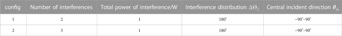
TABLE 2. Typical interference configuration.

Assume that the interference power is equal, and the intersection angle of adjacent interferences are equal. The variation of optimal residual interference power and ICR against the interference distribution and central incident direction is shown in Figure 5. Figures 5(A−D) show the numerical calculation results of configuration ① and configuration ② respectively.

FIGURE 5

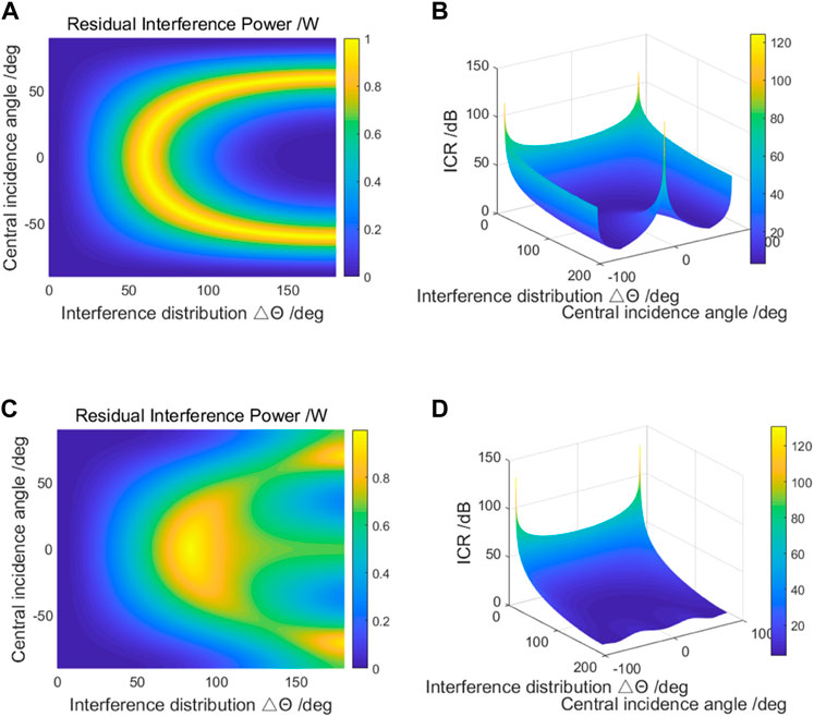
FIGURE 5. The variation of residual interference power and ICR against the interference distribution and central incident direction (two-element array). (A) Optimal residual interference power of config ①; (B) ICR of config ①; (C) Optimal residual interference power of config ②; (D) ICR of config ②.

As shown in Figure 5A, for a two-element array, if the interference number K = 2, the maximum optimal residual interference power is 1 and the minimum value is 0. If the incident direction of interference is symmetrical about ±90°, $\sin {\theta }_{j_k}=\sin \left(\pi -{\theta }_{j_k}\right)=\sin {\theta }_{j_k}$ , thus two interferences are equivalent to one interference. Note that in Figure 5B, ICR should be positive infinity at extreme points, where $\Delta \Theta =0$ and ${\theta }_{j_0}=\pm {90}^{\circ }$. It can be seen from Figures 5C, D that when the interference number K ≥ 2, the maximum value of optimal residual power is less than 1, which shows that it is less effective than two interferences, the analysis at Eq. 47 is verified. For the case of multi element array, if the interference number K ≥ N and the total interference power is 1, it can be either concluded that the maximum optimal residual interference power is 1 (see Appendix B for detailed proof), and the minimum is 0 (according to Section 3.2).

Conclusion 2: If the number of interferences is greater than or equal to the number of array elements, the interference residual power obtained by optimal spatial filter is closely related to the central incident direction and the interference distribution. The maximum value of the interference residual power is the sum of the interference power, and the minimum value is 0. In particular, when the element number N = 2, the maximum residual power equals to the sum of interference power only if the number of interference K = 2.

The above conclusion show that for the evaluation of sup-DOF anti-jamming capability, the interference incidence direction will cause huge differences in the evaluation results, and the anti-interference capability needs to be evaluated separately for different interference deployment scenarios; For the deployment of jammer, if the number and power of several jammer are determined, the interference efficiency can be improved by reasonably setting the incident direction of interference.

4.2 Azimuth periodicity of interference suppression performance

It can be seen from Section 4.1 that in order to study the rule of sup-DOF interference suppression performance, it is necessary to test multiple groups of interference incidence directions, and the workload of simulation calculation is huge. Eq. 45 shows that the interference suppression performance of the linear array takes π as the cycle. If the anti-jamming performance of the plane array also has periodicity, it can reduce the repetitive calculation and improve the simulation efficiency. In order to solve this problem, this section analyzes the periodicity of the interference suppression performance of the navigation receiver array antenna, assuming that the interference signals are independent of each other.

First, take the central UCA of four elements as an example. The element positions are shown in the orange circle in Figure 6, and the coordinates are shown in the Eq. 18.

FIGURE 6

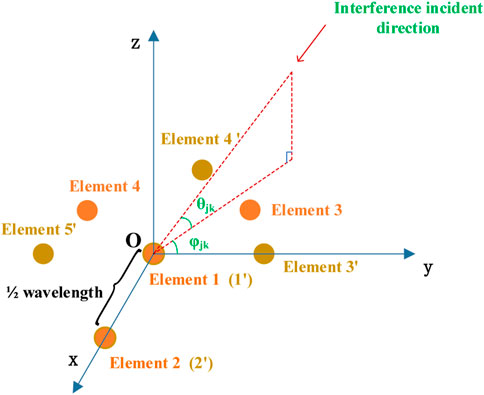
FIGURE 6. Position of array element in Oxyz coordinate system.

Suppose the incident direction in elevation remains constant, if the azimuth angle ${\phi }_{j_k}$ deviates $\frac{2\pi }{3}+\frac{2\pi }{3}m\left(m=0,\pm 1,\pm 2,\cdots \right)$ from the initial direction, then the deviated steering vector is

${\mathbf{a}}_{{\mathbf{j}}_{\mathbf{k}}}^{\prime }=\exp \left\{-\mathrm{j}\frac{\pi }{{\lambda }_c}\cos {\theta }_k\left[\begin{array}{c}0\\ -\sin \left({\phi }_{j_k}+\frac{\pi }{6}\right)\\ \cos \left({\phi }_{j_k}\right)\\ \sin \left({\phi }_{j_k}-\frac{\pi }{6}\right)\end{array}\right]\right\}(49)$

${\mathbf{a}}_{{\mathbf{j}}_{\mathbf{k}}}^{\prime }$ equals to line exchange of ${\mathbf{a}}_{{\mathbf{j}}_{\mathbf{k}}}$, which can be written as follows:

${\mathbf{a}}_{{\mathbf{j}}_{\mathbf{k}}}^{\prime }={\mathbf{T}}_{\mathbf{s}\mathbf{1}}\cdot {\mathbf{a}}_{{\mathbf{j}}_{\mathbf{k}}}(50)$

where ${\mathbf{T}}_{\mathbf{s}\mathbf{1}}$ is the matrix representing row exchange.

${\mathbf{T}}_{\mathbf{s}\mathbf{1}}=\left[\begin{array}{cccc}1& 0& 0& 0\\ 0& 0& 0& 1\\ 0& 1& 0& 0\\ 0& 0& 1& 0\end{array}\right](51)$

${\mathbf{T}}_{\mathbf{s}\mathbf{1}}$ is a unitary matrix, ${\mathbf{T}}_{\mathbf{s}\mathbf{1}}^{\mathbf{H}}={\mathbf{T}}_{\mathbf{s}\mathbf{1}}^{-\mathbf{1}}$.

If all K interferences deviate $\frac{2\pi }{3}+\frac{2\pi }{3}m\left(m=0,\pm 1,\pm 2,\cdots \right)$ relative to the original incident direction, denote ${\mathbf{R}}_{\mathbf{j}\mathbf{j}}^{\prime }$ as the deviated interference covariance matrix. The relationship between ${\mathbf{R}}_{\mathbf{j}\mathbf{j}}^{\prime }$ and the original covariance matrix ${\mathbf{R}}_{\mathbf{j}\mathbf{j}}$ is as follows.

${\mathbf{R}}_{\mathbf{j}\mathbf{j}}^{\prime }={\mathbf{T}}_{\mathbf{s}\mathbf{1}}{\mathbf{R}}_{\mathbf{j}\mathbf{j}}{\mathbf{T}}_{\mathbf{s}\mathbf{1}}^{-1}(52)$

Matrix ${\mathbf{R}}_{\mathbf{j}\mathbf{j}}^{\prime }$ is similar to ${\mathbf{R}}_{\mathbf{j}\mathbf{j}}$, so they have same (smallest) eigenvalues. As a result, this deviation of incident direction in azimuth does not change the optimal residual interference power and ICR.

In the same way, it can be proved that if the azimuth incidence angle deviates $\frac{\pi }{3}+\frac{2\pi }{3}m\left(m=0,\pm 1,\pm 2,\cdots \right)$, the deviated steering vector ${\mathbf{a}}_{{\mathbf{j}}_{\mathbf{k}}}^{″}$ is equal to the line exchange of the conjugate of ${\mathbf{a}}_{{\mathbf{j}}_{\mathbf{k}}}$.

${\mathbf{a}}_{{\mathbf{j}}_{\mathbf{k}}}^{″}={\mathbf{T}}_{\mathbf{s}\mathbf{2}}\cdot {\mathbf{a}}_{{\mathbf{j}}_{\mathbf{k}}}^{*}(53)$

${\mathbf{T}}_{\mathbf{s}\mathbf{2}}=\left[\begin{array}{cccc}1& 0& 0& 0\\ 0& 0& 1& 0\\ 0& 0& 0& 1\\ 0& 1& 0& 0\end{array}\right](54)$

Similarly, if all K interferences are deviated $\frac{\pi }{3}+\frac{2\pi }{3}m\left(m=0,\pm 1,\pm 2,\cdots \right)$ relative to the original incident direction, denote ${\mathbf{R}}_{\mathbf{j}\mathbf{j}}^{″}$ as the deviated interference covariance matrix. The relationship between ${\mathbf{R}}_{\mathbf{j}\mathbf{j}}^{″}$ and the original covariance matrix ${\mathbf{R}}_{\mathbf{j}\mathbf{j}}$ is as follows.

${\mathbf{R}}_{\mathbf{j}\mathbf{j}}^{″}={\mathbf{T}}_{\mathbf{s}\mathbf{2}}{\mathbf{R}}_{\mathbf{j}\mathbf{j}}^{\mathbf{T}}{\mathbf{T}}_{\mathbf{s}\mathbf{2}}^{-1}(55)$

Matrix ${\mathbf{R}}_{\mathbf{j}\mathbf{j}}^{″}$ is similar to ${\mathbf{R}}_{\mathbf{j}\mathbf{j}}^{\mathrm{T}}$. What’s more, the transpose transformation does not change the eigenvalues of the matrix, so the minimum eigenvalue of ${\mathbf{R}}_{\mathbf{j}\mathbf{j}}^{″}$ is the same as that of ${\mathbf{R}}_{\mathbf{j}\mathbf{j}}$. This deviation of incident direction in azimuth does not change the optimal residual interference power or ICR.

To sum up, if the relative relationship between the interference incident directions is certain, the residual interference power of four-element central UCA is periodic in the azimuth direction. The period is $\frac{\pi }{3}$.

Secondly, take the five-element central UCA as an example for analysis. The array element position is shown in the golden circle in Figure 6, where one element is located at the origin, and the other four elements are uniformly distributed on the circumference with half-wavelength radius. By the same derivation method, when the incident direction of the interference is deviated $\frac{\pi }{2}+\frac{2\pi }{3}m\left(m=0,\pm 1,\pm 2,\cdots \right)$ from the original incident direction, the new interference covariance matrix is similar to the original covariance matrix, and the minimum eigenvalue is the same, so the period of the interference residual power is $\frac{\pi }{2}$.

Take the interference number K = 10 as an example to illustrate the numerical calculation of the above analysis results. See Figure 6 for array antenna geometry. Interference parameters are given in Table 3.

TABLE 3

TABLE 3. Jamming configuration.

The relative incident direction of the interference remains constant, and the central incident direction of the azimuth is changed. The changes of residual interference power and ICR against central incident direction in azimuth are shown in Figure 7. Wherein, Figures 7A, B show that the anti-jamming performance period of four-element central UCA is $\frac{\pi }{3}$, while Figures 7C, D show that the anti-jamming performance period of five-element central UCA is $\frac{\pi }{2}$, which verifies the above analysis.

FIGURE 7

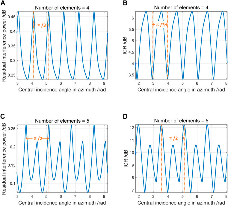
FIGURE 7. Azimuth periodicity of interference suppression performance. (A) Optimal residual interference power of four-element central UCA; (B) ICR of four-element central UCA; (C) Optimal residual interference power of five-element central UCA; (D) ICR of five-element central UCA.

In spite that the central UCA is taken as an example for theoretical derivation and numerical calculation, it can be seen from the derivation process that the azimuth period of the suppression performance is only related to the number of elements uniformly distributed on the circumference, and whether or not to deploy elements at the center of the circle has no effect on the period size. If the number of elements uniformly distributed on the circumference is M (M ≥ 3), it can be further generalized that the interference suppression performance period of UCA or central UCA is.

$\left\{\begin{array}{l}\frac{\pi }{M}\left(Misodd\right)\\ \frac{2\pi }{M}\left(Miseven\right)\end{array}\right.(56)$

Correspondingly, the anti-jamming performance repeats for $N_p$ cycles when the interference azimuth changes from 0 to 2 π towards the central incident direction.

$N_p=\left\{\begin{array}{l}2M\left(Misodd\right)\\ M\left(Miseven\right)\end{array}\right.(57)$

The following conclusion can be further generalized:

Conclusion 3: Assume the interference signals are independent of each other. For an UCA with half-wavelength radius circumference, if the number of elements uniformly distributed on the circumference is M (M ≥ 3), and the number of elements at the center of the circle is 0 or 1, then the interference suppression performance period in azimuth is $\frac{4\pi }{\left.M\cdot {\left(3+(-1\right)}^{M+1}\right)}$. Correspondingly, interference suppression performance repeats ${\left(3+(-1\right)}^{M+1})M/2$ cycles when the central incident direction turns over the range of 2π in azimuth. If the number of elements at the center of the circle is 1, the above conclusion is also applicable to M = 1,2, and the array is degenerated into an ULA (Uniform Linear Array).

This conclusion can be applied to the evaluation of antenna array anti-jamming performance. In the study of the relationship between antenna array anti-jamming performance and azimuth incidence angle, it can reduce the repetitive test or simulation calculation, and improve the evaluation efficiency by ${\left(3+(-1\right)}^{M+1})M/2$ times.

5 Simulation results and analysis

This section verifies conclusion 2 and conclusion 3 through simulation of signal flow.

5.1 Simulation verification of conclusion 2

5.1.1 Simulation scenario 1

Firstly, the theoretical analysis in Section 4.1 is verified by simulation. The simulation parameters are shown in Table 4. Wherein, 1268.52 MHz is the central frequency point of the Beidou navigation system B3I signal. To facilitate comparison with the numerical calculation in Section 4, the total interference power is set as 1 W, and the intersection angles of adjacent interference incident directions are equal.

TABLE 4

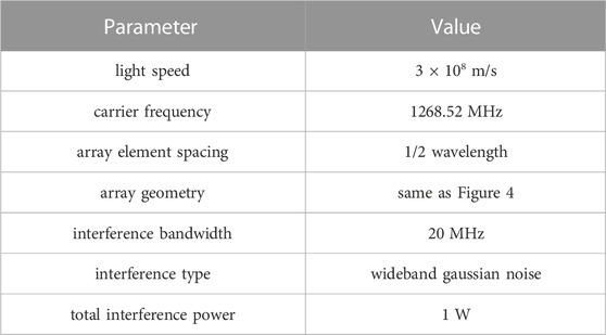
TABLE 4. Settings of simulation parameter.

The variation of anti-jamming performance against central incident direction interference distribution is shown in Figure 8. Four central incident directions are selected for display, and the abscissas are the interference distribution in azimuth and elevation respectively. The simulation verifies conclusion 2. At the same time, it can be concluded from the figure that the anti-jamming performance may be improved by changing the central incident direction and interference distribution of the interference, but the change rule needs to be further studied through statistical data.

FIGURE 8

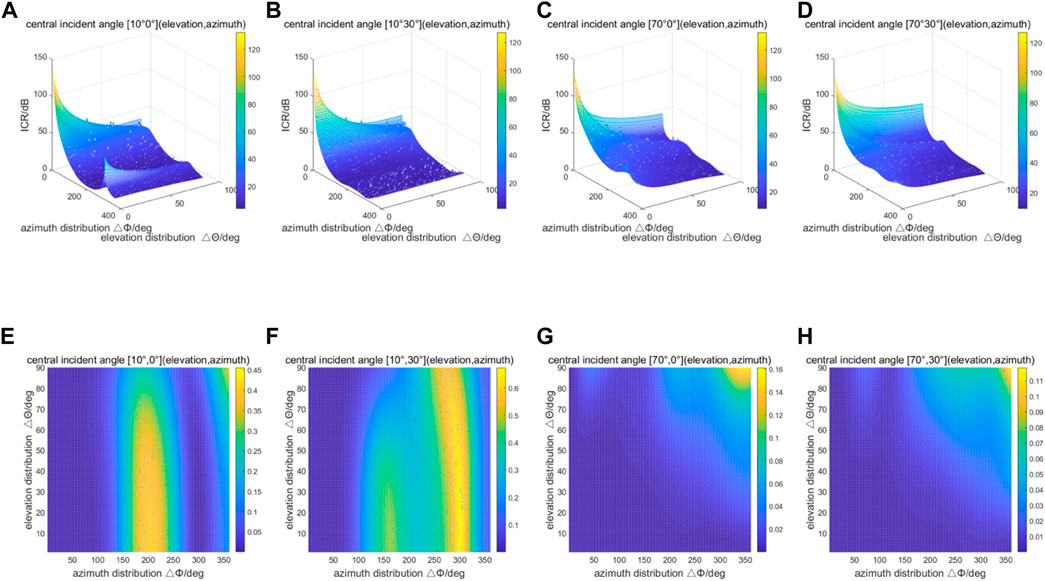
FIGURE 8. Anti-jamming performance against central incident direction and interference distribution. (A) ICR at central incident angle of [10°, 0°]; (B) ICR at central incident angle [10°,30°]; (C) ICR at central incident angle [70°,0°]; (D) ICR at central incident angle [70°,30°]; (E) Optimal residual interference power at central incident angle of [10°,0°]; (F) Optimal residual interference power at central incident angle [10°,30°]; (G) Optimal residual interference power at central incident angle [70°,0°]; (H) Optimal residual interference power at central incident angle [70°,30°].

5.1.2 Simulation scenario 2

Since the number of samples in the above simulation is limited, it fails to verify the statement in conclusion 1 that the maximum of optimal interference residual power is equal to the sum of input interference power. This scenario takes a four-element ULA as an example to illustrate the existence of interference incident directions that accord with the statement.

Assume that the element spacing of the four-element ULA is half wavelength, and the interference number is K. The rest of simulation conditions are the same as those in Table 4. Let the power of interferences be 1/K, and the interference distribution $\Delta {\Theta }_j=\pi$. The distribution meets Eq. 58 while the central incident direction ${\theta }_{j_0}=0$.

${\theta }_{j_k}=\arcsin \left({\alpha }_{j_k}\right)k=\mathrm{1,2},\cdots ,K(58)$

where

${\alpha }_{j_k}=\frac{2k}{K}-1k=\mathrm{1,2},\cdots ,K(59)$

Keep the interference distribution unchanged, take the approximate value K = 10⁵ for simulation, and the relationship between the optimal residual interference power and the interference central incident direction is shown in Figure 9. It can be seen that the residual interference power approaches 1 at ${\theta }_{j_0}=0$. It can be computed that the optimal residual interference power equals to 1 at ${\theta }_{j_0}=0$ while $K\to \infty$. The statement in conclusion 2 that the optimum of residual interference power equals to the sum of input interference power is verified.

FIGURE 9

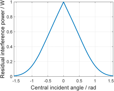
FIGURE 9. Relationship between the optimal residual interference power and the interference central incident direction.

5.1.3 Simulation scenario 3

This scenario simulates and verifies the theoretical analysis in Section 4.2. The initial incident direction parameters and simulation parameters of interference are the same as Tables 3, 4. The simulation results are shown in Figure 10. The horizontal axis in the figure indicates that the azimuth of the interference has varied by 2π from the initial central incident direction, and the vertical axis is the optimal residual interference power of anti-interference processing. The array used in the simulation is a central UCA. According to conclusion 3, when the number of array elements is N = 2, 4, 6, 8, and the number of elements uniformly distributed on the circumference is M = 1, 3, 5, 7, the azimuth period of the interference suppression performance is $\pi$, $\frac{\pi }{3}$, $\frac{\pi }{5}$, $\frac{\pi }{7}$, and the interference suppression performance repeats 2M cycles when the central incident direction turns over the range of 2π; When the number of array elements is N = 3, 5, 7, 9, and the number of array elements uniformly distributed on the circumference is M = 2, 4, 6, 8, the azimuth period of the interference suppression performance is $\pi$, $\frac{\pi }{2}$, $\frac{\pi }{3}$, $\frac{\pi }{4}$, and the interference suppression performance repeats M cycles when the central incident direction turns over 2π in azimuth; The simulation results in Figure 10 verify conclusion 3.

FIGURE 10

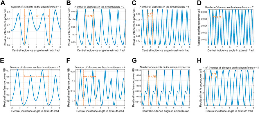
FIGURE 10. Azimuth periodicity (signal flow simulation) of four-element central UCA (A–H).

6 Conclusion

On the condition the number of interference is equal to or greater than the number of array elements, in order to study the anti-jamming capability and mechanism of GNSS array antenna, the following two tasks are completed in this paper: First, the definition of sup-DOF interference for GNSS array antenna is proposed from the perspective of spatial anti-jamming; Secondly, the directional characteristics of GNSS array antenna for sup-DOF interference suppression are analyzed, while numerical calculation and simulation verification are carried out. The main achievements and conclusions are summarized as follows.

(1) The definition of sup-DOF interference is proposed. Accordingly, if the number of interferences is greater than or equal to the number of array elements (K ≥ N), the interference may not surpass the array degree of freedom. The existence of special directions allows the antenna array to completely suppress K interferences.

(2) If the number of interferences is greater than or equal to the number of array elements, the value of the interference residual power obtained by optimal spatial filter is closely related to the central incident direction and the interference distribution. The maximum value of the interference residual power is the sum of the interference power, and the minimum value is 0.

(3) Assume the interference signals are independent of each other. For an UCA with half-wavelength radius circumference, if the number of elements uniformly distributed on the circumference is M (M ≥ 3), and the number of elements at the center of the circle is 0 or 1, then the interference suppression performance is periodic. The interference suppression performance repeats $N_p$ cycles when the central incident direction turns over the range of 2π in azimuth.

$N_p=\left\{\begin{array}{l}2M\left(Misodd\right)\\ M\left(Miseven\right)\end{array}\right.(60)$

7 Discussion

The conclusion of this paper gives the upper and lower bounds of the sup-DOF interference suppression capability for typical GNSS antenna arrays, and derives the azimuthal periodic rule of the sup-DOF interference suppression capability. The former item has guiding significance for the jammer DOA deployment. The latter one can be useful in interference suppression performance evaluation, which improves the evaluation efficiency by ${\left(3+(-1\right)}^{M+1})M/2$ times. The conclusions are drawn basically on narrowband array signal model, while it can be proved that they are also tenable for wideband model. The future work includes studying the relationship between interference suppression capability and power, number, direction and distribution of jammers, and to conclude detailed quantitative results.

Data availability statement

The original contributions presented in the study are included in the article/Supplementary Material, further inquiries can be directed to the corresponding author.

Author contributions

YS performed the theoretical study, conducted the simulations, and wrote the manuscript; FC provided the methodology and revised the manuscript; FW provided conceptualizations and research suggestions; WL and BL helped with programming and revised the manuscript; JS helped in figures and correction. All authors have read and agreed to the published version of the manuscript.

Funding

This research was supported in part by the Natural Science Foundation of China (NSFC), grants No. 62003354.

Acknowledgments

The authors would like to thank the editors and reviewers for their efforts in supporting the publication of this paper.

Conflict of interest

The authors declare that the research was conducted in the absence of any commercial or financial relationships that could be construed as a potential conflict of interest.

Publisher’s note

All claims expressed in this article are solely those of the authors and do not necessarily represent those of their affiliated organizations, or those of the publisher, the editors and the reviewers. Any product that may be evaluated in this article, or claim that may be made by its manufacturer, is not guaranteed or endorsed by the publisher.

References

1. Kaplan ED, Hegarty CJ. GPS principle and application. Beijing, China: Electronic Industry Press (2002). p. 1.

Google Scholar

2. Kohno R, Imai H, Hatori M, Pasupathy S. Combinations of an adaptive array antenna and a canceller of interference for direct-sequence spread-spectrum multiple-access system. IEEE J Sel Areas Commun (1990) 8:675–82. doi:10.1109/49.54463

CrossRef Full Text | Google Scholar

3. Bei D. Navigation satellite system open service performance standard. Available from: http://www.beidou.gov.cn/xt/gfxz/202105/P020210526216231136238.pdf.

Google Scholar

4. Morton YTJ, van Diggelen F, Spilker JJ, Parkinson BW, Lo S, Gao G. Position, navigation, and timing technologies in the 21st century, Vol. 1. Piscataway, NJ, USA: Wiley-IEEE Press (2020). p. 1121.

Google Scholar

5. Gupta IJ, Weiss IM, Morrison AW. Desired features of adaptive antenna arrays for GNSS receivers. Proc IEEE (2016) 104:1195–206. doi:10.1109/JPROC.2016.2524416

CrossRef Full Text | Google Scholar

6. Wang J, Ou G, Liu W, Chen F. Characteristic analysis on anti-jamming degrees of freedom of GNSS array receiver. In: Proceedings of the 13th China satellite navigation conference. Beijing, China: CSNC (2022). p. 463.

CrossRef Full Text | Google Scholar

7. Fernandez-Prades C, Arribas J, Closas P. Robust GNSS receivers by array signal processing: Theory and implementation. Proc IEEE (2016) 104:1207–20. doi:10.1109/JPROC.2016.2532963

CrossRef Full Text | Google Scholar

8. Jie W, Wenxiang L, Feiqiang C, Zukun L, Gang O. GNSS array receiver faced with overloaded interferences: Anti-jamming performance and the incident directions of interferences. J Syst Eng Electron (2022) 6:1–7. doi:10.23919/JSEE.2022.000072

CrossRef Full Text | Google Scholar

9.Gstar anti-jam gps—electronic protection. Available from: https://www.lockheedmartin.com/content/dam/lockheed-martin/rms/documents/electronic-warfare/GSTAR%20Brochure.pdf (accessed on 25 April 2022).

Google Scholar

10.GPS Anti-Jam. Available from: https://www.mayflowercom.com/us/technology/gps-anti-jam/(accessed on April 25, 2022).

11. Mitch RH, Dougherty RC, Psiaki ML, Steven PP. Signal characteristics of civil GPS jammers. In: Proceedings of the proceedings of the 24th international technical meeting of the satellite division of the Institute of navigation. Portland, OR, USA (2011). (ION GNSS 2011).

Google Scholar

12. Abdulkarim Y, Xiao M, Awl H, Muhammadsharif F, Lang T, Saeed S, et al. Simulation and lithographic fabrication of a triple band terahertz metamaterial absorber coated on flexible polyethylene terephthalate substrate. Opt Mater Express (2022) 12:338–59. doi:10.1364/OME.447855

CrossRef Full Text | Google Scholar

13. Gu Y, Goodman NA. Information-theoretic compressive sensing kernel optimization and bayesian cramér–rao bound for time delay estimation. IEEE Trans Signal Process (2017) 65:4525–37. doi:10.1109/TSP.2017.2706187

CrossRef Full Text | Google Scholar

14. Moffet A. Minimum-redundancy linear arrays. IEEE Trans Antennas Propag (1968) 16:172–5. doi:10.1109/TAP.1968.1139138

CrossRef Full Text | Google Scholar

15. Xu Y, Liu Z, Gong X. Signal processing of polarization sensitive array. Beijing, China: National Defense Industry Press (2013).

Google Scholar

16. Ojeda OAY, Grajal J, Lopez-Risueño G. Analytical performance of GNSS receivers using interference mitigation techniques. IEEE Trans Aerosp Electron Syst (2013) 49:885–906. doi:10.1109/TAES.2013.6494387

CrossRef Full Text | Google Scholar

17. Manikas A, Proukakis C, Lefkaditis V. Investigative study of planar array ambiguities based on “hyperhelical” parameterization. IEEE Trans Signal Prosessing (1999) 47(6):1532–41. doi:10.1109/78.765122

CrossRef Full Text | Google Scholar

18. Vandana AR, Jaysaval VK, Reddy CRB. Enhancement of unambiguous DOA estimation for phase comparison monopulse radar. Proc 2015 Int Conf Adv Comput Commun Inform (Icacci) (2015) 10-:1165. doi:10.1109/ICACCI.2015.7275768

CrossRef Full Text | Google Scholar

19. Pan G, Wang L, Hua J. Anti-jamming technology of satellite navigation receiver. Beijing, China: Electronic Industry Press (2016). p. 181.

Google Scholar

20. Potts D, Tasche M, Volkmer T. Efficient spectral estimation by MUSIC and ESPRIT with application to sparse FFT. Front Appl Maths Stat (2016) 2. doi:10.3389/fams.2016.00001

CrossRef Full Text | Google Scholar

21. Frank A, Cohen I. Constant-beamwidth kronecker product beamforming with nonuniform planar arrays. Front Signal Process (2022) 2. doi:10.3389/frsip.2022.829463

CrossRef Full Text | Google Scholar

22. Lu Z, Nie J, Chen F, Chen H, Ou G. Adaptive time taps of STAP under channel mismatch for GNSS antenna arrays. IEEE Trans Instrum Meas (2017) 66:2813–24. doi:10.1109/TIM.2017.2728420

CrossRef Full Text | Google Scholar

23. Sun Y, Chen F, Lu Z, Wang F. Anti-jamming method and implementation for GNSS receiver based on array antenna rotation. Remote Sens (2022) 14:4774. doi:10.3390/rs14194774

CrossRef Full Text | Google Scholar

Appendix A

It proves that in Eq. 47, the equality of $p_{jres,\max }\le {\displaystyle \sum }_{k=1}^K{p}_{j_k}$ is obtained at K = 2. Eq. 47 is given below.

$p_{jres}={\displaystyle \sum }_{k=1}^K{p}_{j_k}-\sqrt{{\left({\displaystyle \sum }_{k=1}^K{p}_{j_k}\right)}^2-2{\displaystyle \sum }_{\underset{u\ne v}{u=1,v=1}}^K{p}_{j_u}{p}_{j_v}\left(1-\cos \left(\pi \sin {\theta }_{j_u}-\pi \sin {\theta }_{j_v}\right)\right)}$

Proof

If the total interference power is fixed, ${\displaystyle \sum }_{k=1}^K{p}_{j_k}=p_{jtot}$ is a fixed value. To maximize the interference residual power, the root term of the above equation needs to take the minimum value. This problem is equivalent to the following optimization problem:

$\left\{\begin{array}{l}\underset{p_1,p_2}{\min }{\displaystyle \sum }_{k=1}^K{p}_{j_k}^2+{\displaystyle \sum }_{\underset{u\ne v}{u=1,v=1}}^K{p}_{j_u}{p}_{j_v}{\mathrm{e}}^{\mathrm{j}\pi \sin {\theta }_{j_u}-\mathrm{j}\pi \sin {\theta }_{j_v}}+{\displaystyle \sum }_{\underset{u\ne v}{u=1,v=1}}^K{p}_{j_u}{p}_{j_v}{\mathrm{e}}^{\mathrm{j}\pi \sin {\theta }_{j_v}-\mathrm{j}\pi \sin {\theta }_{j_u}}\\ s.t.{\displaystyle \sum }_{k=1}^K{p}_{j_k}=p_{jtot}\end{array}\right.(\mathrm{A1})$

Denote

$\mathbf{p}=\left[\begin{array}{c}{p}_{j_1}\\ p_{j_2}\\ ⋮\\ p_{j_k}\end{array}\right](\mathrm{A2})$

$\mathbf{H}=\left[\begin{array}{cccc}1& {\mathrm{e}}^{\mathrm{j}\pi \sin {\theta }_{j_1}-\mathrm{j}\pi \sin {\theta }_{j_2}}& \cdots & {\mathrm{e}}^{\mathrm{j}\pi \sin {\theta }_{j_1}-\mathrm{j}\pi \sin {\theta }_{j_v}}\\ {\mathrm{e}}^{\mathrm{j}\pi \sin {\theta }_{j_2}-\mathrm{j}\pi \sin {\theta }_{j_1}}& 1& \cdots & {\mathrm{e}}^{\mathrm{j}\pi \sin {\theta }_{j_2}-\mathrm{j}\pi \sin {\theta }_{j_v}}\\ ⋮& ⋮& \ddots & ⋮\\ {\mathrm{e}}^{\mathrm{j}\pi \sin {\theta }_{j_u}-\mathrm{j}\pi \sin {\theta }_{j_1}}& {\mathrm{e}}^{\mathrm{j}\pi \sin {\theta }_{j_u}-\mathrm{j}\pi \sin {\theta }_{j_2}}& \cdots & 1\end{array}\right](\mathrm{A3})$

Let $\left|{\theta }_{j_1}\right|<\left|{\theta }_{j_2}\right|<...<\left|{\theta }_{j_k}\right|$, then the above problem is a convex optimization problem of quadratic form, namely

$\left\{\begin{array}{l}\underset{\mathbf{p}}{\min }{\mathbf{p}}^{\mathbf{H}}\mathbf{H}\mathbf{p}\\ s.t.{\mathbf{p}}^{\mathbf{H}}\mathbf{b}=p_{jtot}\end{array}\right.(\mathrm{A4})$

among them $\mathbf{b}={\left[\begin{array}{cc}1& 1\end{array}\right]}^T$.

It can be solved that when $0°<{\theta }_{j_1,}{\theta }_{j_2},\dots ,{\theta }_{j_k}<90°$ or $-90°<{\theta }_{j_1},{\theta }_{j_2},\dots ,{\theta }_{j_k}<0°$, the optimal value of interference power deployment is

${\mathbf{p}}_{\mathbf{o}\mathbf{p}\mathbf{t}}=\left[\begin{array}{c}{p}_{j_{tot}}/2\\ 0\\ ⋮\\ 0\\ p_{j_{tot}}/2\end{array}\right](\mathrm{A5})$

herein

${\displaystyle \sum }_{k=1}^K{p}_{j_k}^2+{\displaystyle \sum }_{\underset{u\ne v}{u=1,v=1}}^K{p}_{j_u}{p}_{j_v}{\mathrm{e}}^{\mathrm{j}\pi \sin {\theta }_{j_u}-\mathrm{j}\pi \sin {\theta }_{j_v}}+{\displaystyle \sum }_{\underset{u\ne v}{u=1,v=1}}^K{p}_{j_u}{p}_{j_v}{\mathrm{e}}^{\mathrm{j}\pi \sin {\theta }_{j_v}-\mathrm{j}\pi \sin {\theta }_{j_u}}=0(\mathrm{A6})$

It can be proved that when the range of ${\theta }_{j_1},{\theta }_{j_2},\dots ,{\theta }_{j_k}$ is $\left|{\theta }_{j_k}-{\theta }_{j_1}\right|\ge 90°$, the optimal value of interference power deployment has the following form

$\left\{\begin{array}{l}{p}_{j_u}=p_{j_v}=\frac{p_{tot}}{2}\\ p_{j_{k|k\ne u,v}}=0\end{array}\right.(\mathrm{A7})$

This is equivalent to that the maximum value of interference residual power is obtained when the interference number K = 2.

Appendix B

It proves that in Section 4.1, if the number of array elements N > 2, The optimal residual interference power is the sum of input interference power.

Proof

Denote ${\mathrm{C}}^N$ as N-dimensional complex vector space. Assume the total power of interference is 1, the steering vectors of K (K ≥ N) interferences is $\begin{array}{cccc}{\mathbf{a}}_{{\mathbf{j}}_{\mathbf{1}}}& {\mathbf{a}}_{{\mathbf{j}}_{\mathbf{2}}}& \cdots & {\mathbf{a}}_{{\mathbf{j}}_{\mathbf{K}}}\end{array}$ respectively (not linearly correlated), the power of which is $\begin{array}{cccc}{p}_{j_1}& p_{j_2}& \cdots & p_{j_K}\end{array}$, and the initial phase is $\begin{array}{cccc}{\gamma }_{j_1}& {\gamma }_{j_2}& \cdots & {\gamma }_{j_K}\end{array}$. The element space constructed by interferences is

$S_e=\left\{\begin{array}{cccc}{p}_{j_1}\exp \left(\mathrm{j}{\gamma }_{j_1}\right){\mathbf{a}}_{{\mathbf{j}}_{\mathbf{1}}}& p_{j_2}\exp \left(\mathrm{j}{\gamma }_{j_2}\right){\mathbf{a}}_{{\mathbf{j}}_{\mathbf{2}}}& \cdots & p_{j_K}\exp \left(\mathrm{j}{\gamma }_{j_K}\right){\mathbf{a}}_{{\mathbf{j}}_{\mathbf{K}}}\end{array}\right\}(\mathrm{B1})$

Denote the complex number

${\beta }_{j_k}=p_{j_k}\exp \left(\mathrm{j}{\gamma }_{j_k}\right)k=\mathrm{1,2},\cdots ,K(\mathrm{B2})$

Since K ≥ N and the steering vectors are not linearly correlated, there are ${\beta }_{j_k}$ ($k=\mathrm{1,2},\cdots ,K$) that confirms

$S_e=Span\left\{\begin{array}{cccc}{\mathbf{a}}_{{\mathbf{j}}_{\mathbf{1}}}& {\mathbf{a}}_{{\mathbf{j}}_{\mathbf{2}}}& \cdots & {\mathbf{a}}_{{\mathbf{j}}_{\mathbf{N}}}\end{array}\right\}=Span\left\{\begin{array}{cccc}{\mathbf{a}}_{{\mathbf{j}}_{\mathbf{1}}}& {\mathbf{a}}_{{\mathbf{j}}_{\mathbf{2}}}& \cdots & {\mathbf{a}}_{{\mathbf{j}}_{\mathbf{K}}}\end{array}\right\}(\mathrm{B3})$

Considering

$Span\left\{\begin{array}{cccc}{\mathbf{a}}_{{\mathbf{j}}_{\mathbf{1}}}& {\mathbf{a}}_{{\mathbf{j}}_{\mathbf{2}}}& \cdots & {\mathbf{a}}_{{\mathbf{j}}_{\mathbf{K}}}\end{array}\right\}=\left\{\mathbf{a}|\mathbf{a}={\beta }_1{\mathbf{a}}_{{\mathbf{j}}_{\mathbf{1}}}+{\beta }_2{\mathbf{a}}_{{\mathbf{j}}_{\mathbf{2}}}+\cdots +{\beta }_K{\mathbf{a}}_{{\mathbf{j}}_{\mathit{K}}}\right\}={\mathrm{C}}^N(\mathrm{B4})$

It is evident that there is ${\beta }_{j_k}$ ($k=\mathrm{1,2},\cdots ,K$) that confirms

$S_e={\mathbf{I}}_{\mathbf{N}}(\mathrm{B5})$

where ${\mathbf{I}}_{\mathbf{N}}$ is the unit matrix. Herein, the minimum eigenvalue is 1, so the maximum of optimal residual interference power is 1. In other words, the optimal residual interference power is the sum of input interference power.