On the effect of the thermal cross-talk in a photonic feed-forward neural network based on silicon microresonators

Local heating is widely used to trim or tune photonic components in integrated optics. Typically, it is achieved through the power dissipation of metal microwires driven by a current and placed nearby the photonic component. Then, via the thermo-optic effect, both the amplitude and the phase of the complex optical field propagating in the component can be controlled. In the last decade, optical integrated circuits with a cascade of more than 60 thermo-optical phase shifters were demonstrated for quantum simulators or optical neural networks. In this work, we demonstrate a simple two layers feed-forward neural network based on cascaded of thermally controlled Mach-Zehnder interferometers and microring resonators. We show that the dynamics of a high quality factor microresonator integrated into a Silicon On Insulator (SOI) platform is strongly affected by the current flowing in metal heaters where these last generate both local as well as global heating on the integrated photonic circuit. Interestingly, microheaters, even when they are at distances of a few millimetres from the optical component, influence all the microresonators and the Mach-Zehnder interferometers in the photonic circuit. We model the heat flux they generate and modify accordingly the non-linear equations of a system formed by a microresonator coupled to a bus waveguide. Furthermore, we show experimentally that the use of microheaters can be a limiting factor for the feed-forward neural network where three microresonators are used as non-linear nodes. Here, the information encoding, as well as the signal processing, occurs within the photonic circuit via metal heaters. Specifically, the network reproduces a given non-linear surjective function based on a domain of at most two inputs and a co-domain of just one output. As a result, its training aims to determine the values of the currents to apply to the heaters in the hidden layers, which allows replicating a certain shape. We demonstrate how the network exploits mainly the heat flow generated by the information encoding to reproduce a target avoiding the use of all the hidden layer heaters. This work shows that in large thermally actuated integrated photonic circuit, the thermal cross talk is an issue.

1 Introduction

In integrated photonics, microheaters are used to locally change the temperature and, via the thermo-optic effect, the refractive index. Thus, they influence the phase of the propagating optical field forming a photonic component named phase-shifter. In particular, the engineering of phase-shifters in a photonic circuit allows implementing any linear spatial optical transformations [1]. As a result, microheaters are used to create reconfigurable integrated photonic circuits when the operational speed is not demanding. In recent decades, advancements in integrated photonics have made possible the realization of high-performance non-resonant Silicon thermo-optic phase shifters. Consequently, large-scale programmable photonic processors based on thermally controlled Mach-Zhender Interferometers (MZI), where phase shifters are integrated in the MZI arms, have been realized. These have paved the way for novel implementations in quantum photonics information processing [2, 3], in optical communications (through large-scale low-loss optical switches) [4], and in machine learning [1, 5].

Despite the breakthroughs in energy efficient Silicon thermo-optic phase shifters, they have a limitation in their operational speed. Typically, the thermo-optic time constant can span from few μs to about 70 μs [4, 6–9]. As a result, a steady state of the system is ensured by working at tens of kHz. This limits their use in applications, e.g., in photonic neural network. In fact, the training of a feed-forward network based on a cascade of programmable MZIs can be time consuming. In these large arrays, the speed is not the only limitation. Indeed, it was observed a heat flow through the substrate caused by a thermo-optic modulator array [10, 11]. Consequently, a microheater not only changes the local temperature of the component to which it is interfaced but also influences the overall chip temperature by a heat flow through the substrate. This latter can affect the response of components that are far away and strongly impact the achievement of a steady state in the photonic circuit. Typically, this thermal cross-talk introduces phase perturbations across the circuit and delays to reach the steady state. The impact of the global heat flow through the substrate is particularly relevant in the case of microresonators or of unbalanced MZIs. Microresonators with high-quality (high-Q) factors show shift in their resonance wavelength of up to about 70 pm/K due to a temperature variation [6]. The presence of a distant microheater can affect the spectral position of the microresonator resonance via the heat flow in the substrate. The same could happen in an unbalanced MZI, where the different arm lengths induce a phase-shift term due to the thermal cross-talk between distinct phase-shifters.

Over the years, both, structural solutions [12–15] and control methods [11, 16, 17], have been proposed to mitigate the thermal cross-talk in the presence of MZIs and microresonators. However, as far as we know, a study of the influence of local and global temperature variations on the non-linear response of microresonators is lacking. Here, “local” refers to the temperatures of single photonic components, such as the microheater or microresonator. On the other hand, “global” refers to the temperature of large regions of the whole optical circuit which includes the substrate temperature as well as is affected by the variations of local ones. We model and verify how the heat generated both locally and globally by microheaters influences the dynamics of high-Q microresonators integrated in a Silicon On Insulator (SOI) photonic circuit. Precisely, we model the variation caused by the heat flux on the non-linear equations of a microresonator/bus waveguides system. Furthermore, we experimentally show the limitations of the use of microheaters as phase-shifters in a feed-forward neural network with microresonators as non-linear activation functions. Here, the information encoding as well as the signals processing is performed in the integrated photonic circuit by means of phase-shifters actuated by microheaters. Training is achieved in supervised learning by minimizing a cost function through a free gradient algorithm. The manuscript is organized as follows. In Section 2, we introduce the theoretical model and the experimental measurements on the thermal cross-talk between a microresonator and a far microheater. In Section 3, we discuss a feed-forward neural network where the thermal cross-talk influences the overall network performances. Finally, we sum up our results in Section 4.

2 Modeling the global heating influence on the microresonator response

2.1 Theoretical model development

Let us consider a silicon microresonator coupled to two bus waveguides in the add and drop configuration (see Figure 1A). The non-linear response of the system is due to either or both the dynamics of the free carrier population density and of the temperature in the ring waveguide [18]. A strong field intensity generates free carriers through Two Photon Absorption (TPA). These, in turn, induce the free carrier dispersion, and, consequently, a decrease of the effective waveguide index, i.e., a blue shift of the microresonator’s resonant frequencies. Meanwhile, the temperature of the microresonator increases because of the free carrier relaxation and light absorption in the waveguide. As a result, the microresonator’s resonant frequencies red shift due to the thermo-optic effect. These two non-linear phenomena, which generate a contrasting shift of the resonant frequencies, are characterized by different relaxation times and power dependence [19]. Therefore, as a function of the input field and the boundary conditions, one can exploit one or both non-linear effects. In the latter case, the dynamics are characterized by an unstable regime due to the self-pulsing effect [20]. These non-linearities were recently used to demonstrate a reservoir computing network by using a single microresonator and time multiplexing [21, 22].

FIGURE 1

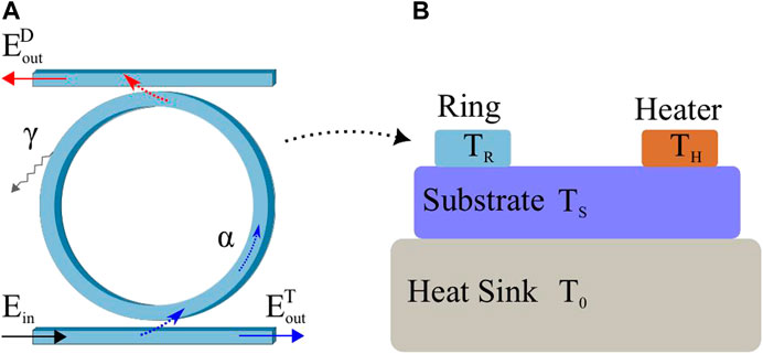
FIGURE 1. (A) Sketch of a microresonator in the add and drop configuration. (B) Sketch of the four blocks used to model the heat exchange between the microheater and the microresonator. The different symbols are defined in the text.

The temporal dynamics of a silicon microresonator can be modeled by three coupled ordinary differential equations (23). These govern the field amplitude propagating inside the microresonator α, the free carrier population ΔN and the temperature difference between the waveguide core and the cladding ΔT [19, 23]:

$\frac{\mathrm{d}\alpha }{\mathrm{d}t}=i{\omega }_0\left(1+\delta \right)\alpha -\gamma \alpha +i\sqrt{2{\gamma }_e}{E}_{in},(1)$

$\frac{\mathrm{d}\mathrm{\Delta }N}{\mathrm{d}t}=-\frac{\mathrm{\Delta }N}{{\tau }_{fc}}+g_{\text{TPA}}{\left|\alpha \right|}^4,(2)$

$\frac{\mathrm{d}\mathrm{\Delta }T}{\mathrm{d}t}=-\frac{\mathrm{\Delta }T}{{\tau }_{th}}+\frac{P_{\text{abs}}}{m{c}_p},(3)$

$\begin{array}{ll}\hfill \delta & =-\frac{1}{n_0}\left[\frac{\mathrm{d}n}{\mathrm{d}T}\mathrm{\Delta }T+{\sigma }_{\text{FCD}}\mathrm{\Delta }N+n_2{\left|\alpha \right|}^2\right],\hfill \\ \hfill \gamma & =2{\gamma }_e+{\gamma }_i+{\eta }_{\text{FCA}}\mathrm{\Delta }N+{\eta }_{\text{TPA}}{\left|\alpha \right|}^2.\hfill \end{array}(4)$

The definitions and values of the parameters in these equations are reported in the first section of the supplementary material. Here, it suffices to say that δ is the dimensionless resonance shift; γ_e is the damping rate due to extrinsic losses (we assume two equal coupling rates for the top and bottom waveguides), γ is the damping rate due to the total loss (extrinsic plus the intrinsic γ_i losses). E_in is the electric field at the input of the microresonator. The output electric field at the through port is $E_{\mathit{out}}^T=E_{in}+i\sqrt{2{\gamma }_e}\alpha$, and consequently, at the drop one is $E_{\mathit{out}}^D=i{e}^{i\pi m}\sqrt{2{\gamma }_e}\alpha$, where $m\in \mathbb{N}$ is the mode order of the microresonator. The exponential term in $E_{\mathit{out}}^D$ takes into account the relative phase of the even and odd microresonator’s modes. The absorbed power is P_abs = 2(γ−2γ_e)|α|². The non-linear transient phenomena occur at time scales related to the thermal relaxation time (τ_th) and the free carrier lifetime (τ_fc). An estimation of these values is given in [19]: τ_fc ≃ 45 ns and τ_th ≃ 280 ns. Note that a rigorous estimation of this latter requires a more complex formulation than Eq. 3. Such a formulation goes beyond the simple approximation of Newton’s law of cooling. Since here we are interested in modeling the influence of a microheater on the linear and non-linear response of a microresonator, the time scale of the system’s temporal dynamics makes Eq. 3 an excellent approximation.

In order to model the interaction between a microheater and a distant microresonator, let us consider the system depicted in Figure 1B. It consists of four blocks: the microresonator which is physically distant from the microheater, the substrate and the heat sink. Each of them is characterized by a temperature, labeled T_R, T_H, T_S and T₀, respectively. Here, T_R and T_H are the local temperatures, while T_S is a global temperature which rules the global thermal flux. Our simple theoretical model is based on the heat exchange between these four blocks. The propagation of heat by conduction within the system can be formalized by the Newton’s law of cooling [24]. As a result, one re-writes Eq. 3 in terms of T_R, and adds two differential equations for T_H and T_S:

$\frac{\mathrm{d}{T}_{\text{R}}}{\mathrm{d}t}=\frac{P_{\text{abs}}}{C_{\text{R}}}-\frac{{\tilde{k}}_1}{C_{\text{R}}}\left(T_{\text{R}}-T_{\text{S}}\right),(5)$

$\frac{\mathrm{d}{T}_{\text{H}}}{\mathrm{d}t}=\frac{P_{\text{c}}}{C_{\text{H}}}-\frac{{\tilde{k}}_2}{C_{\text{H}}}\left(T_{\text{H}}-T_{\text{S}}\right),(6)$

$\begin{array}{ll}\hfill \frac{\mathrm{d}{T}_{\text{S}}}{\mathrm{d}t}& =\frac{{\tilde{k}}_1}{C_{\text{S}}}\left(T_{\text{R}}-T_{\text{S}}\right)+\frac{{\tilde{k}}_2}{C_{\text{S}}}\left(T_{\text{H}}-T_{\text{S}}\right)\hfill \\ \hfill & -\frac{{\tilde{k}}_3}{C_{\text{S}}}\left(T_{\text{S}}-T_0\right).\left(7\right)\hfill \end{array}$

Here, ${\tilde{k}}_1$, ${\tilde{k}}_2$ and ${\tilde{k}}_3$ are the coefficients that quantify the heat exchange between the interfaces created by the microresonator/substrate, heater/substrate, and substrate/heat-sink, respectively. These coefficients are proportional to the heat exchanged per unit time and temperature, and are proportional to the contact area between the two surfaces of the blocks. C_R, C_H and C_S are the heat capacities of the microresonator, heater, and substrate, respectively. The latter can be expressed as the product of the mass times the specific heat as in Eq. 3, where C_R = mc_p. P_c is the driving term of Eq. 6 and is the electrical power supplied to the microheater. Within this simple model, the thermal relaxation time assumes the following expression ${\tau }_{th}=C_{\text{R}}/{\tilde{k}}_1$. Similarly, we can define the heater relaxation time and the cross-talk time as ${\tau }_{\text{H}}=C_{\text{H}}/{\tilde{k}}_2$ and ${\tau }_{\text{CT}}=C_{\text{S}}/{\tilde{k}}_3$. Note that Eq. 4 for δ remains unchanged. However now, ΔT is the difference between the actual temperature of the microresonator (T_R) and the temperature of the “cold” microresonator (T₀). T₀ is the temperature at which the cold resonant frequency (ω₀) is measured with a low input power laser, i.e., in the linear regime.

Eqs 5, 6 show that the microresonator and the microheater exchange heat through the substrate. As a result, τ_CT rules the action of the microheater on the microresonator and vice versa. Here, with the term substrate we mean the material between the microresonator and the heat sink: it can be just the bare wafer substrate, or even the package, when the chip is placed in a ceramic handler. The heat sink is usually formed by a metal (commonly copper) maintained at a constant temperature (T₀) through a Peltier cell. Furthermore, our model assumes that the substrate block has a uniform temperature. This means that there is no temperature difference between the substrate region close to the microresonator and the one near the microheater. Neglecting the temperature inhomogeneity within every single block is a strong approximation justified by the fact that we are interested in the thermal cross-talk between the microheater and the microresonator at relatively large distances. This assumption means that τ_H is an effective average characteristic time that takes into account also the time required for the heat to spread in the substrate region near the microheater. A more rigorous description of this system would have required to consider the temperature variation within each material of each block. However, the model would have been very elaborate and computationally demanding, without giving relevant advantages on the description of the global thermal cross-talk.

2.2 The linear response and the estimation of τ_CT and τ_H

In the linear regime, τ_CT and τ_H can be estimated through the optical response. In this case, |α|² ≪ 1, and, consequently, P_abs ≃ 0 and ΔN ≃ 0. As a result, Eq. 2 does not play any role and T_R is only governed by T_S (Eq. 5). To compute the thermal times, we use as initial conditions a hot microheater (T_H ≠ 0) with no current (P_c[t ≥ 0] = 0), and a constant temperature of the heat sink T₀ = cost = 0. In this case, the thermal differential equations can be solved analytically. In fact, since ${\tilde{k}}_1/C_{\text{R}}=1/{\tau }_{th}\gg ({\tilde{k}}_1+{\tilde{k}}_2+{\tilde{k}}_3)/C_{\text{S}}$, they reduce to:

$T_{\text{R}}=T_{\text{S}},(8)$

$T_{\text{H}}=T_{\text{S}}+\left(T_{\text{H}}\left[0\right]-T_{\text{S}}\left[0\right]\right)e^{-\frac{t}{{\tau }_{\text{H}}}},(9)$

$T_{\text{S}}=A{e}^{-\frac{t}{{\tau }_{\text{CT}}}}+B{e}^{-\frac{t}{{\tau }_{\text{H}}}},(10)$

where T_H[0] and T_S[0] are the temperatures at t = 0 of the microheater and the substrate, respectively. A and B are constants, which assume the following expression:

$\begin{array}{ll}\hfill A& =T_{\text{S}}\left[0\right]\left(1-\frac{C_{\text{H}}{\tilde{k}}_2}{C_{\text{H}}{\tilde{k}}_3-C_{\text{S}}{\tilde{k}}_2}\right)-\frac{T_{\text{H}}\left[0\right]C_{\text{H}}{\tilde{k}}_2}{C_{\text{H}}{\tilde{k}}_3-C_{\text{S}}{\tilde{k}}_2},\hfill \\ \hfill B& =\frac{\left(T_{\text{H}}\left[0\right]-T_{\text{S}}\left[0\right]\right)C_{\text{H}}{\tilde{k}}_2}{C_{\text{H}}{\tilde{k}}_3-C_{\text{S}}{\tilde{k}}_2}.\hfill \end{array}$

It is observed that the solutions Eqs 8–10 represent a thermalization of the system to T₀ with different relaxation times. Using Eqs 4, 8, 10 one can directly connect the resonance frequency shift (δ) of the microresonator to the exponential drop of T_S:

$\delta =-\frac{1}{n_0}\left[\frac{\mathrm{d}n}{\mathrm{d}T}\left(A{e}^{-\frac{t}{{\tau }_{\text{CT}}}}+B{e}^{-\frac{t}{{\tau }_{\text{H}}}}\right)\right].(11)$

When 1/τ_H ≫ 1/τ_CT, δ depends on τ_CT only.

To measure τ_CT and τ_H, let us consider a microresonator point-coupled to two bus waveguides in the add and drop configuration with a gap of 250 nm. The microresonator has a ring shape with a radius of 7 μm and consists of a Si waveguide with a cross-section of 450 nm × 220 nm embedded in silica cladding and fabricated at the IMEC/Europractice facility within a multi-project wafer (MPW) run. The microheaters consists of straight stripes made in titanium nitride (TiN) with a length of about 60 μm and a width of approximately 6 μm. Hereunder, we used two different systems: a chip within a ceramic electronic packaging (named packaged chip) and a chip without the electronic packaging and directly mounted on the chip metallic holder (bare chip). The used optical setup has a fiber-coupled continuous wave tunable laser (Yenista OPTICS, TUNICS-T100S) interfaced to a polarization control stage. The laser signal is coupled to the optical chip by using two single-mode stripped fibers via grating couplers. The alignment is ensured by two x-y-z piezo-positioners stages. The optical response is detected by means of a photodiode detector (Thorlabs, PDA10CS2) and it is recorded with an 3 GHz oscilloscope (LeCroy wavepro 7300A). Both the packaged and the bare chips are placed on a thermostat holder whose temperature is controlled through a Proportional-Integral-Derivative controller (SIM960 Analog PID controller) via a Peltier cell and a 10 kΩ thermistor. A write-board (Measurement Computing USB-3106), with an amplification stage, applies and controls the current to the microheaters.

Let us consider the experimental results in the case of the packaged chip in the linear regime. Figure 2a1 shows the microresonator transmittance as a function of the frequency detuning Δω measured at the through port when the microheater is off (i.e., the temperatures are all equal to the substrate temperature). First, the input frequency was fixed at the point given by the red cross in (a1) and the microheater was turned on by applying a constant current until a steady state is reached. Then the current was switched off, and the time dependence of the transmission was measured (red lines of Figures 2a2–a4). The different transmission decays refer to the microresonator thermalization for three different distances (d_HR) from the microheater of 1275 μm (a2), 655 μm (a3) and 240 μm (a4), respectively. Each of these exponential decays has been fitted by assuming a Lorentzian microresonator spectral response [25, 26]:

$T\left[\mathrm{\Delta }\omega \right]=1-\frac{4{\gamma }_e\left(\gamma -{\gamma }_e\right)}{\mathrm{\Delta }{\omega }^2+{\gamma }^2},(12)$

where Δω = ω−ω₀δ−ω₀ and ω is the frequency of the input laser signal. In this case, an excellent fit for the time responses is obtained by fixing B = 0 in Eq. 11 (black lines in Figure 2). From the fit, we obtain τ_CT = (204.7 ± 3.2) ms, (215.8 ± 2.2) ms and (215.1 ± 1.1) ms for panels (a2), (a3) and (a4), respectively. Noteworthy, τ_CT does not depend significantly on d_HR.

FIGURE 2

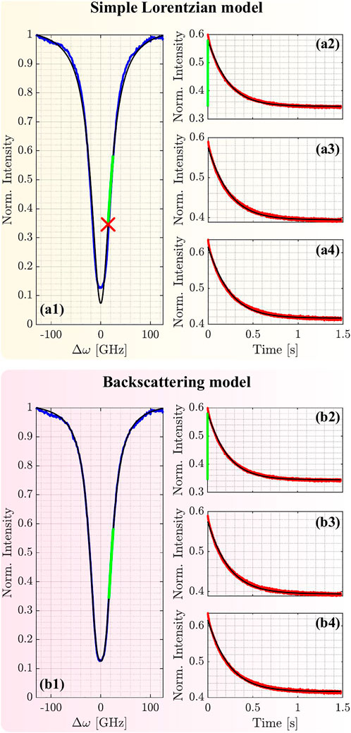
FIGURE 2. Microresonator in the packaged chip. (a1) transmission of the through port as a function of the detuning Δω. The blue line is the experimental data, the red cross is the spectral position of the input signal for the time decay experiments of (a2–a4), the green line refers to the spectral shift observed during the microresonator cooling, the black line is a fit with a simple Lorentzian model. (a2–a4) transmission intensity as a function of time after the switch-off of the current driving the microheater placed at a distance of 1275 μm, 655 μm and 240 μm, respectively. Red lines refer to the experimental data, black lines to the fit curve. (b1–b4) show the same experimental data as (a2–a4) but fit with a different model which takes into account backscattering effects.

We can conclude that the temperature of the microresonator is not affected by the variation of d_HR. This justifies a posteriori the assumption in the model on the temperature homogeneity of the three blocks (Figure 1). However, this assumption is valid only for large distances between the microheaters and the microresonator, i.e., for d_HR > 200 μm. Indeed, as shown in [27] the temperature gradient near the microheaters is not negligible.

The fit by the Lorentzian shape, Figure 2a1, misses the experimental results close to zero detuning. This is due to the surface-wall roughness that generates counter-propagating modes [28]. A more accurate modeling yields [28, 29]:

$T\left[\mathrm{\Delta }\omega \right]={\left|1-\frac{2{\gamma }_e\left(-i\mathrm{\Delta }\omega +\gamma \right)}{{\left(-i\mathrm{\Delta }\omega +\gamma \right)}^2-{\beta }^2{e}^{i\varphi }}\right|}^2,(13)$

with the backscattering coefficients β and ϕ. Figures 2b1–b4 show the fit results. The excellent agreement yields τ_CT = (213.2 ± 3.4) ms, (221.5 ± 2.4) ms and (220.3 ± 1.0) ms for (b2), (b3) and (b4), respectively. These values are comparable with those obtained by using Eq. 12.

The studied microresonator has a quality factor of about 2.6 × 10⁴. It is sensitive to the temperature change of the microheater even at a distance of about 1.3 mm. The estimated τ_CT shows that a relaxation time of about 1.5 s is required to thermalize the microresonator at its cold state, i.e., at T₀.

Performing the same measurements on the bare optical chip, the cooling speeds-up. Figure 3, shows the results. Here, the fit with Eq. 13 yields τ_CT = (22.1 ± 2.9) ms, i.e., one order of magnitude lower than that of the packaged chip. Note that in this case, both exponentials in Eq. 11 were used. This allows estimating τ_H = (3.1 ± 1.1) ms. This value is much longer than the one usually assumed of about ≃ 70 μs [4] and it is in agreement with the present model in which we defined an effective average characteristic time. For the bare optical chip, the cold state is reached in about 100 ms (see Figure 3). The difference between the bare and packaged chip is due to the ceramic package and its large heat capacity.

FIGURE 3

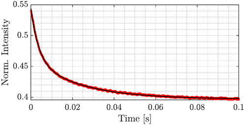
FIGURE 3. Experimental decay of the transmission intensity at the through port of a microresonator in the bare optical chip after turning off the current to the microheater. The red line shows the experimental data, while the black line the fit with the model. The data refer to the similar experiment reported in (b4) of Figure 2 for the packaged chip, i.e., a distance between the microresonator and the microheater of about 240 μm.

Section two of the supplementary material reports the fitting parameter values.

2.3 The non-linear response

In the non-linear regime, the heat exchange between the microheater and the microresonator through the substrate can induce an unstable regime. This can be modeled by fixing proper initial conditions on the pump laser frequency (ω_p) and on the microheater current. In particular, one must: (i) turn on the heater at a constant current, (ii) scan slowly ω_p toward the resonance, starting from the right shoulder of the Lorentzian reported in Figure 2. Here, by slowly we mean that the ω_p scan is done by keeping a stationary regime for the microresonator, i.e., after a change in ω_p the microresonator is permitted to relax to a new stationary state. Then, the microheater current is turned off. As a consequence, the microresonator relaxes (see Figure 2) and its resonance shifts can trigger a self-pulsing phenomenon by the thermal cross-talk. An example is shown in Figure 4 for the packaged chip: Figures 4a1–a3 report the through port transmittance as a function of time. Here, the microresonator is about 1275 μm far from the microheater which was switched off at t = 0. It is observed that the signal decay at t = 0 (Figure 4a2) and, then, a selpulsing regime sets-in after about 120 ms (Figure 4a3).

FIGURE 4

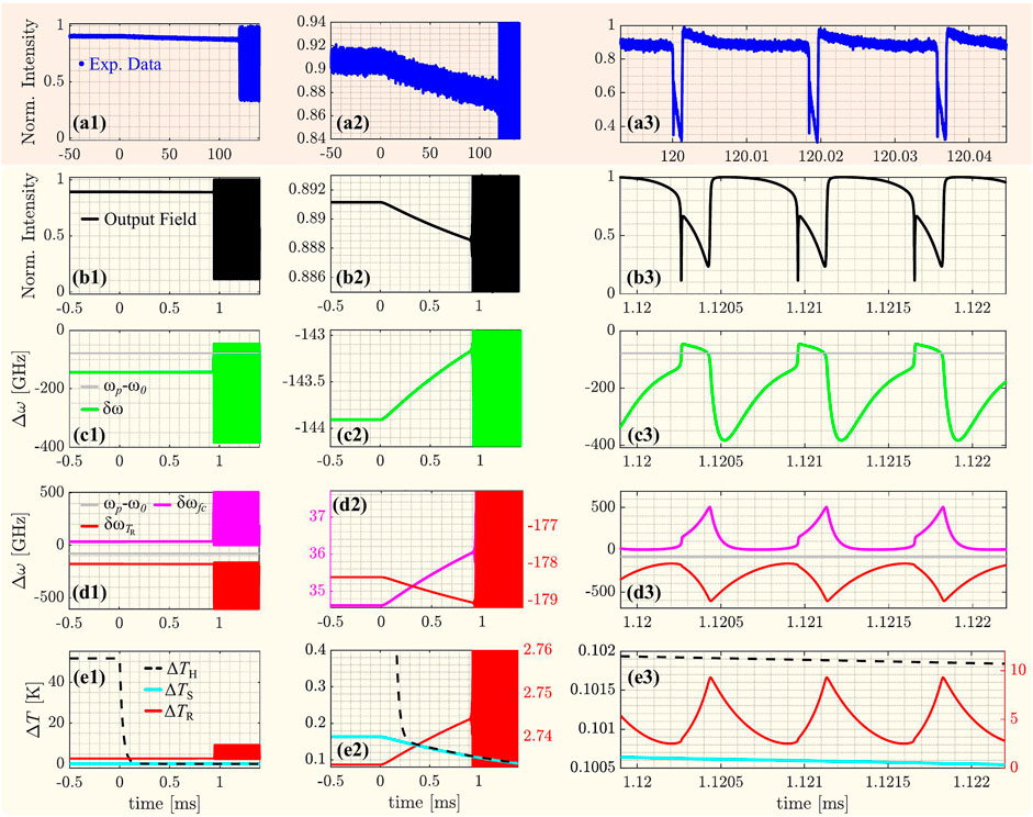
FIGURE 4. Microresonator through port transmission in the non-linear regime and for ω_p shifted of about −80 GHz with respect the cold resonance. Panels (a1–a3) show the experimental data for the packaged chip. (a2) is a blow-up of (a1) on the intensity scale. (a3) is a blow-up of (a1) in the time interval around 120 ms. (b1–b3) to (e1–e3) refer to the numerical simulation results. (b1–b3) report the simulated through signal (black lines). (c1–c3) display the resonance shift δω as a function of time (green line). ω_p is shown as the gray horizontal line. (d1–d3) show the resonance shift due to the free carriers concentration (δω_fc, pink line) and due to the variation of the microresonator temperature ($\delta {\omega }_{T_{\text{R}}}$ red line), separately. (e1–e2) show the time evolution of the temperature difference between the microresonator temperature and T₀ (ΔT_R, red line), the microheater temperature and T₀ (ΔT_H, dashed black line), the substrate temperature and T₀ (ΔT_S, light blue line). For clarity in panel (d2) the curves are represented through two y-axes: one left in pink to show δω_fc and one right in red to show $\delta {\omega }_{T_{\text{R}}}$. The same for (e2) and (e3) where the left axis in black is related to ΔT_S and ΔT_H while the right red axis is related to ΔT_R.

Taking advantage of the ODE 23 algorithm of MATLAB^®, we have solved the differential equations of our model (Eqs 1, 2, 5, 6, 7). Due to the finite available computation power, we have scaled all the typical times by two orders of magnitude. In this way, using a PC equipped with an Intel^® Core™ i5-11500 and 32 GB RAM, the computational time is about 1.5 h with respect of about 6.3 days with the real time scale. The numerical results are shown in Figures 4b1–e3. Modeling follows the experimental procedure to drive the microresonator into the self-pulsing regime. The parameters used are reported in the supplementary materials. Figure 4b2 shows an exponential decay of the transmitted intensity that starts when the microheater is turned off, i.e., t = 0. Notably, when the thermal cross talk via the substrate moves the resonance frequency close enough to ω_p, fast and intense oscillations are observed due to the self-pulsing regime (Figure 4b3). A comparison between the experimental data (Figures 4a1–a3) and the simulated data (Figures 4b1–b3) shows that the model is able to grasp the major trends in the experiments. Therefore, we look at the temporal lineshapes of the various relevant quantities.

Figures 4c1–c3 show the temporal dependence of the resonance shift (δω = δ ⋅ ω₀). For t < 0, δω is constant.

At t > 0, δω exponentially approaches ω_p. This δω increase is caused by the substrate temperature and ends when the microresonator enters into the self-pulsing regime where δω oscillates around (ω_p−ω₀) (Figure 4c3). In this regime, when the hot resonance is resonant with the pump, the density of free carrier is so large that the free carrier effects overcome the thermo-optic effect. Then, δω decreases and the free carrier population rapidly decreases. At this point, the thermo-optic effect dominates and the process restarts: this causes the self-pulsing oscillations. Note that the initial shift occurs with τ_CT as characteristic time constant, while the fast self-pulsing dynamics is defined by τ_th and τ_fc (Figure 4c3).

Figures 4d1–d3 show the separated effects on δω due to the variation of the microresonator temperature $(\delta {\omega }_{T_R})$ and of the free carriers (δω_fc). Figures 4e1–e3 show the differences between the temperature of the “cold” microresonator and the actual temperatures ΔT_j = T_j−T₀ (j = H, S, R) of the microheater (black dashed line), substrate (cyan line) and microresonator (red line). When t < 0 all the temperatures are constant, i.e., the system is in a stationary state. At t = 0, the microheater is switched off and its temperature rapidly decreases to the substrate temperature (Figure 4e1). Figures 5A, B show a zoom of Figures 4d2, e2, respectively. It shows that at t = 0 the turning off the microheater induces a decrease of ΔT_R, and therefore, an increase of $\delta {\omega }_{T_{\text{R}}}$. Then, after few tenths of μs, T_R increases which causes in turn a $\delta {\omega }_{T_{\text{R}}}$ decreases. The reason for this is the interplay between the free carrier effect, the thermo-optic effect, and the global heating related to the cross talk. In fact, the cooling of the substrate moves the resonant frequency to the blue which causes an increase of the free carrier concentration. The free carrier effect brings (δω+ω₀) closer to the pump laser frequency (Figures 4d2, c2) which in turn induces an increase in the temperature of the microresonator. The free carrier effect overcomes the thermo-optic one and grows with τ_CT. This slow behavior is due to the fact that both the free carrier concentration and the microresonator temperature are in a stationary state at the time scale of the slowly substrate temperature decrease. In fact, this latter is the driving force of the resonance frequency shift toward the blue.

FIGURE 5

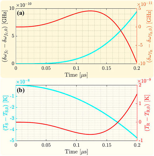
FIGURE 5. Panels (A) and (B) report respectively a zoom of Figure 4 (d2) and (e2) when the microheater is switched off. For the seek of clarity, the graphs show the quantity $[\delta {\omega }_{fc}-\delta {\omega }_{fc,t=0},\delta {\omega }_{T_{\text{R}}}-\delta {\omega }_{T_{\text{R}},t=0}]$ and [T_S−T_{S, t=0}, T_R−T_{R, t=0}]. Two different y-axes (left and right) are used in graphs (A,B). In (A) pink (left axis) and red (right axis) for δω_fc and $\delta {\omega }_{T_{\text{R}}}$, respectively. In (B) cyan (left axis) and red (right axis) for T_S and T_R, respectively.

When the temperature of the microresonator and the free carriers concentration reach the threshold, the self-pulsing is established, and the substrate no longer dominates the dynamics. In fact, as seen in Figure 4e3, the temperature change associated with the unstable regime leads ΔT_R to oscillate between 3 and 10 K. During these fast oscillations, the substrate temperature decreases only slightly.

Summarizing, we demonstrated that self-pulsing in a microresonator can be caused by switching off a microheater 1.3 mm far. This can be described by our theoretical model, which catches the physics of both the temperature variation and the non-linear optical behavior. As a result, the variation of the local microresonator’s temperature (typically influenced only by the driving optical signal) is linked to that of far microheaters through the heat flow in the substrate of the system. As already mentioned, our intuitive model neglects the local temperature gradients in regions close to both the microheater and microresonator. Therefore, it does strictly describe the effect of the global thermal cross-talk only when the distances between microheaters and microresonators are larger than 200 μm.

3 The global heating influence on a photonic feed-forward neural network

The results of the previous section show that the use of microheaters to make phase-shifters is not as simple as initially thought. Indeed, the heat induced by the microheater has fast local dynamics and slow global dynamics which influence the linear and non-linear properties of photonic components far in space. Let us see how this impacts on a photonic feed-forward neural network (FFNN).

3.1 Experimental sample and optical setup

Three microresonators are used as neurons within a simple two layers FFNN (Figure 6A). The FFNN has been fabricated within the same MPW run as the microresonators discussed in Section 2.2. The FFNN has an input preparation layer, where the data are encoded, two hidden layers, and an output layer. In the input layer, the input signal (In) is coupled via a grating coupler (G_in,0). Then, it is split into two waveguides via a balanced 1 × 2 Multi-Mode Interferometer (MMI) splitter. As a result, two input signals pass through two equal arms, labeled as Top and Bottom in Figure 6A. These are characterized by a nearly-balanced MZI followed by a phase shifter (PS). On one arm of the MZI is placed a TiN microheater, which allows tuning the refractive index. By the current values (in_1,1 and in_2,1), the interference at the output of the MZIs is controlled which in turn controls the amplitude of the MZIs transmitted signal. Then, the signal passes through a phase shifter (PS). Control taps collect 5% of the signals (output at G_in,1 and G_in,2). Therefore, in the input layer, an incoming coherent beam is divided into two, and data (x₁ and x₂) are encoded in the amplitude and the phase of the transmitted fields.

FIGURE 6

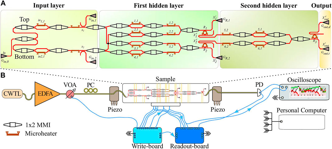
FIGURE 6. (A) Design of the feed-forward neural network. It consists of four parts: an input layer where the information is encoded, a first/second hidden layer where the input data is processed, and finally, an output layer to record the network’s response. The red lines show the silicon waveguides, the brown ones the integrated heaters, while the black components the balanced 1 × 2 or 2 × 1 Multi-Mode Interferometers (MMIs). The three non-linear microresonators play the role of the active nodes. Labels and numbers on the design are explained in the text. (B) Sketch of the experimental setup. CWTL: Continuous Wave Tunable Laser, EDFA: Erbium Doped Fiber Amplifier, VOA: Variable Optical Attenuator, PC: Polarization Control and PD: Photodiode. Details are explained in the text.

x₁ and x₂ enter the first hidden layer. Each one is split in two along four different arms where a MZI and a PS allow manipulation of their amplitude and phase. Then, two balanced MMIs recombine two by two the signals by mixing the ones elaborated in the top branch with those of the bottom branch. Then, these two signals are coupled to the R₁ and R₂ microresonators. The microresonators have a ring shape with a radius of 7 μm and they are point-like coupled to two bus waveguides in the add and drop configuration with a gap of 210 nm. The estimated quality factor is approximately 1.4 × 10⁴ at 1570.5 nm. The through signals of each microresonator are outcoupled via grating couplers (G_R,1 and G_R,2) to monitor the microresonator response at the through port ($X_1^{\prime }$ and $X_2^{\prime }$).

The signals at the exit of the first hidden layer are the transmissions at the drop ports of the two microresonators. They can be written as:

$\begin{array}{lll}\hfill X_j^{\text{d}}\left(t\right)& =f_{R_j}^{\text{d}}\left(\sum _{n=1}^2{x}_n\left(t\right)\right.\hfill & w_{\left(j^2-j+n\right),1}{w}_{\left(j^2-j+n\right),2}),\hfill \end{array}$

where j labels the two microresonators, $f_{R_j}^{\text{d}}$ are their response functions, w_k,1 is the weight applied by the k-th MZI and w_k,2 by the k-th PS. More specifically, the weights applied by the MZIs assume the expression $\frac{1}{2}(1+e^{i\mathrm{\Delta }\mathrm{\Phi }})$, while those related to the PSs are written as e^iΔθ. In both cases, the arguments of the exponential (ΔΦ and Δθ) are given by the microheaters’s temperature variation (ΔT) as $L\frac{2\pi }{\lambda }\frac{\mathrm{d}n}{\mathrm{d}T}\mathrm{\Delta }T$, where λ is the signal wavelength, L is the length of the metal strip in the microheater and $\frac{\mathrm{d}n}{\mathrm{d}T}$ is the silicon thermo-optic coefficient.

In the second hidden layer, the two input signals are weighted by a series of a MZI and a PS and, then, they are recombined by a MMI at the output. The resulting signal couples to a third microresonator (R₃). This latter also has a ring shape with a radius of 7 μm and it is point-like coupled to two bus waveguides in the add and drop scheme but with a gap of 240 nm. For this microresonator, the estimated quality factor is about 1.8 × 10⁴ at 1570.5 nm. The through and the drop signals are then extracted by two grating couplers (G_out,t and G_out,d) that yield the response of the FFNN:

$X_{\mathit{out}}^{\text{t/d}}\left(t\right)=f_{R_3}^{\text{t/d}}\left(\sum _{n=1}^2{X}_n^{\text{d}}\left(t\right)w_{\left(n+4\right),1}{w}_{\left(n+4\right),2}\right).$

Note that since the through and the drop ports of the microresonator are closely related by the energy conservation, the final output consists of a single signal.

All three microresonators have a microheater placed on their external rim, and therefore, their resonant frequency can be thermally tuned. Consequently, the FFNN has nineteen integrated heaters (orange lines in Figure 6) which are wire bonded to the package of the chip. It is worth noting that the distance between the MZIs of the input layer and the microresonators of the first hidden layer is about 795 μm. On the other hand, the gap between the MZIs of the input layer and the output microresonator is even larger, about 1288 μm.

The FFNN was tested with the experimental setup sketched in Figure 6B. The light source is a fiber-coupled continuous wave tunable laser (Yenista OPTICS, TUNICS-T100) operating in the infrared range (1470 nm—1580 nm). The generated CW signal passes through an erbium doped fiber amplifier (EDFA), an electrically controlled variable optical attenuator (VOA) and a polarization control stage. Then, it is coupled via a single mode stripped fiber in the FFNN circuit by means of a grating coupler. At the output of the device, another single mode stripped fiber collects the transmission signal and sends it to an InGaAs photodetector (Thorlabs, PDA20CS2). A correct alignment of the input and output fibers is ensured by a three axis linear piezoelectric stage. The temperature of the optical chip is thermostated through a Peltier cell, which fixed T₀. A readout-board (Measurement Computing USB-2408) and an 3 GHz oscilloscope (LeCroy wavepro 7300A) record the signal of the detector. A write-board (Measurement Computing USB-3106) controls the currents that drive the microheaters in the FFNN and the voltage that is applied to the VOA. The outputs of the write-board are also acquired by the readout-one board and monitored by the oscilloscope. A personal computer allows remote controlling of the different instruments and processes the oscilloscope traces.

3.2 Task to solve and information encoding

We test the capability of our FFNN in the classification of non-linear datasets by looking at its capability in defining non-linear decision boundaries [1]. The task consists in forming linear and non-linear shapes by fixing the boundaries between two-levels, which are encoded by the 0 and 1 bits. Precisely, the input layer of the network generates a two-dimensional intensity matrix contained in ${\mathbb{R}}^2$ that corresponds to the domain set. This is associated with a peculiar intensity vector of the output field, namely the target co-domain which is contained in $\mathbb{R}$. The FFNN training aims at the determination of the weight vector (W) capable of replicating a given shape in the given domain set. Hence, the weights define a specific surjective function, which reproduces the target.

The input domain set is defined by a grid formed by two intensity vectors ${\left|{\mathbf{x}}_1\right|}^2$ and ${\left|{\mathbf{x}}_2\right|}^2$ of a defined length n. It is built by varying the weights ($w_{i{n}_1,1}$ and $w_{i{n}_2,1}$) produced by the input MZIs, namely the in_1,1 and in_2,1 currents which drive the PS in the input MZIs (Figure 6). In this way, the signal intensities x₁ and x₂ at the output of the input layer are changed in the given input domain set. The resulting measured intensities tapped by the gratings G_in,1 and G_in,2 are shown in Figures 7A, B. Here, we show the normalized intensities as a function of the square of the currents applied to the microheaters. The data are all normalized to the peak value recorded at the output of G_in,1, i.e., 1 corresponds to the same intensity value for both x₁ and x₂ signals. Figures 7A, B show that the data (points) follow the typical response of a MZI, which is fitted by a cosine function (1/2 + cos[ΔΦ]/2) as shown by the red curves. The discretization and, therefore, the creation of the domain set, consists of linearly dividing the intensities ${\left|{\mathbf{x}}_1\right|}^2$ and ${\left|{\mathbf{x}}_2\right|}^2$, starting from 1 and setting a minimum threshold of about 20% of the maximum intensity. Here, we show results obtained with n = 6, i.e., a 6 × 6 square input matrix. Hence, this process leads to the grid represented in Figures 7A, B with the black horizontal and blue vertical lines.

FIGURE 7

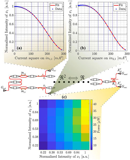
FIGURE 7. (A) The normalized intensity x₁ (blue data points) as a function of the square current in_1,1 applied to the microheater which controls the phase shifter in the first MZI. The red line fits the data with the MZI response. The black vertical and blue horizontal lines define the discretized points used to build the domain set. (B) same as (A) for x₂. The inset shows a sketch of the neural network with evidenced the gratings from which the different experimental data are collected. (C) The output co-domain as a function of the input domain set. It is built by measuring the untrained neural network transmission.

The domain set corresponds to a given co-domain obtained by measuring the response of the whole network at the output grating (G_out,t). In this way, each pair of values defined by the vectors ${\left|{\mathbf{x}}_1\right|}^2$ and ${\left|{\mathbf{x}}_2\right|}^2$, labeled as (x_1,j, x_2,k), corresponds to only one intensity of the output field. The measure of the response of the network to the input matrix is shown in Figure 7C where the map of the output signal intensity is reported as a function of the normalized input intensities, i.e., ${\left|{\mathbf{x}}_1\right|}^2$ and ${\left|{\mathbf{x}}_2\right|}^2$. The measurements are done with the input signal frequency resonant to the R₁ and R₂ microresonator resonant frequencies, while R₃ is kept out of resonance. Consequently, we measured low values of the output for low values of the input and vice versa. However, there are values of the input signals where the linear response of the microresonators affects the output intensity values in the untrained FFNN. As an example, one can note that the input values $\left(\mathrm{1,0.84}\right)$ exhibit a higher value of the associated output intensity with respect to the pair $\left(\mathrm{1,1}\right)$. Note that the pairs created by the discretization process, are passed from the input to the hidden layers according to a defined temporal sequence.

3.3 The cost function

The training consists in setting the weight vector W of the FFNN in order to realize the task. The suitable weight vector is found by minimization of a cost function $(C\left(\mathbf{W}\right))$. We choose $C\left(\mathbf{W}\right)$ in order to maximize the difference between the 0 and 1 bit levels which are distributed in the set according to the specific shape given by the task. This choice focuses on the worst case scenario contained in the output vector of the co-domain $({\mathbf{X}}_{\mathit{out}}^{\text{t/d}})$. Specifically:

$C=\underset{\forall bit0}{\max }{\mathbf{X}}_{\mathit{out}}^{\text{t/d}}\left(\mathbf{W}\right)-\underset{\forall bit1}{\min }{\mathbf{X}}_{\mathit{out}}^{\text{t/d}}\left(\mathbf{W}\right).(14)$

In the training process, the currents of six MZIs, of four PSs, of three microresonators (i.e., of 13 microheaters) are varied. In this way, the setting of the w_1,1, w_2,1, w_3,1, w_4,1, w_1,2, w_4,2, $w_{R_1}$, $w_{R_2}$, w_5,1, w_6,1, w_5,2, w_6,2, and $w_{R_3}$ elements of the weight vector is achieved. Note that not all the PS are independent and are therefore used (eg., and with reference to the labels in Figure 6, the 2,2 and 3,2 PS are not used because their effect is compensated by the 1,2 and 4,2 PS).

3.4 Non-linear task and supervised learning

We tested the FFNN on several shapes, both as simple as vertical stripes or more complex such as geometrical figures. Let us discuss a non-linear task which consists in learning a square shape. This task includes a geometric boundary that cannot be identified linearly, i.e., by a straight line. Consequently, it requires a non-linear response of the hidden layers and/or output one of the FFNN (see Figure 8A).

FIGURE 8

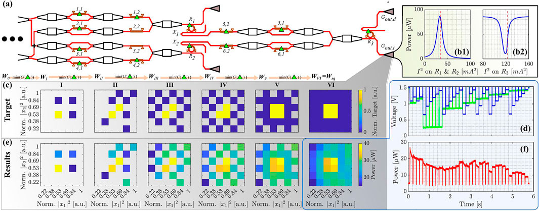
FIGURE 8. (A) sketch of the first and second hidden layers of the feed-forward network with the used microheaters evidenced by the green triangles. Each microheaters is labeled by the index of the weight matrix. (b1) Output signal intensity (collected out of the G_out,t grating) as a function of the square of the currents of the microheaters R₁ and R₂. The dashed red line highlights the initial working points of the microresonators. (b2) Output signal intensity as a function of the square of the current of the microheater R₃. (C) Sequence of the different sub-tasks which lead to the final target, i.e., the square shape. (D) Temporal sequence of the voltages applied to the microheaters of the input layer (in_1,1 -blue line- and in_2,1 - green line) to form the domain set. (E) Experimental maps of the output response after the training for the different sub-tasks described by panel (C). (F) Time sequence of the output signals for the co-domain of map VI in panel (E).

In the training process, the initial state is defined by recording the output of the network (Figures 8b1, b2) and set the currents close to maximum transmission for R₁ and R₂ and to the minimum transmission for R₃. This setting is indicated in Figures 8b1, b2 by the dashed red vertical line. The initial working point is selected to get most of the input signal coupled to the microresonators, and therefore, to exploit their non-linearity. During the training, also the voltage applied to the VOA can be changed which means that the network can adjust the node activation function to the proper working point, either by varying the spectral position of the microresonators (here are the microheaters on the microresonator which play a role) or by changing the input signal power (here is the voltage of the VOA which plays a role).

Since we use a large number of weights (13 in the FFNN and 1 in the VOA) to solve a difficult non-linear tasks, the use of genetic algorithms, such as the particle swarm algorithm, makes the training unreasonably long. In fact, the number of interactions and the time to create a single output matrix lead to an average training time of about 1 day. During this time, the optical setup misalignes due to mechanical relaxation of the fiber holders and other unwanted external perturbations. Therefore, we used a supervised clustering training method. This is based on dividing the task into a sequence of progressively more complex sub-tasks and using the output of the previous sub-task as starting weights for the training of the next substask. Then, by a free gradient algorithm, namely fminsearch of the MATLAB^® packet, we solve the i−th sub-task and use the solution as the initial condition of the i−th+1 sub-task. (see Figure 8C).

Figure 8C shows the application of this method to the square shape target task: on a 6 × 6 matrix we want four central elements equal to 1 and the remaining 32 equal to zero. In the first sub-task (I), four elements are used, of which three are zero and just one is one. In the second (II), the total number of elements increases to 9, with 2 equal to 1 and the remaining 7 zero. Then, the other sub-tasks get more complex until the target. The position of the elements in the different sub-tasks, as well as the corresponding digital value is chosen in order to optimize the minimization of the cost function. In the training process, the 36 values of the domain set are generated and used as input to the hidden layers following a given temporal sequence. Specifically, the pairs of currents corresponding to the positive elements are always processed before the pairs corresponding to the zero elements. In addition, the values of the pairs are always generated row by row starting from right to left and from top to bottom. The voltages used to generate the (x₁(t), x₂(t)) pairs are shown as a function of time in Figure 8D. Here, the blue line corresponds to x₁(t), while the green line corresponds to x₂(t). A whole domain map is created in about 6 s. In the training process, for each sub-task the network elaborates the information in the following way: sets the weights, processes the entire set of the current pairs, accumulates the output signal as a function of time (see, e.g., Figure 8F), calculates the cost function, re-sets the weights, and restart the iteration. This cycle ends when a limit value of the cost function is reached or at a specified number of iterations. A guard time of about 3 s is used between each entire set of the current pairs. During this pause, the maximum current is applied to the microheaters of the input MZIs to minimize the optical response. This allows the optical field within the FFNN to be damped and thus to re-establish the initial conditions of the microresonator.

3.5 Experimental results and role of thermal cross-talk

For each sub-task, the training is verified by the graph of the sub-domain map it generates (Figure 8E). Each map displays the measured output signal powers obtained by processing the matrix of input current pairs through the obtained vector of weights. The experimental measurements show a clear difference between bits 1 and 0: i.e., the network has solved the task to learn a square shape. As a comparison, the similar map for the unlearned network is shown in Figure 7C. The supervised training process takes about 20 min to move from the first sub-task (I) to the final target (VI). More in detail, the time sequence of the output intensity signals for a fixed weight matrix is shown in Figure 8F. The first four levels correspond to the four positive elements that generate the square in map VI. Whereas the remaining 32 levels are the zero elements that complete the co-domain. Note that the network training leads to a temporal shape characterized by a higher power for the four first elements than the others.

This is made possible by the exponential decay that characterizes the power of the positive elements. This trend is determined by the dynamics of the microresonators. Looking at the vector of weights determined by the training procedure, we note that the only non-zero currents are for those which drive the heaters of the microresonators: $w_{R_1}$, $w_{R_2}$ and $w_{R_3}$. More importantly, the exponential time constant characteristics of the output signal is equal to the cross-talk relaxation time as measured in the packaged chip (see Section 2.2). Indeed, a quasi-plateau is reached at the end of the fourth positive element at about 1 s. Consequently, the square shape is generated mainly by the interaction between the heaters in the input layer (characterized by the currents in_1,1 and in_2,1) and the three microresonators of the hidden layers. A role is also played by the VOA which is set during the training to an input laser power yielding a stable non-linear regime of the microresonators, i.e., not in the self-pulsing regime. Noteworthy, by setting the weights of the training and inserting x₁ and x₂ into the hidden layers not following the specific sequence but randomly, the network is no longer able to reproduce the target. Even, by re-training the network the task is not achieved.

In fact, the FFNN moves the microresonators resonant frequency to make use of the global heating induced during the guard time. During this time, the inputs are heated to their maximum value, so as soon as the input sequence begins the average current through the microresonator heaters decreases causing a decrease of the substrate temperature. As a result, the first non-zero element in the temporal sequence exhibit a higher optical power with respect to the later zero ones. This can be evidenced by solving another task, such as the one shown in Figure 9. Here, a “O” and an “F” shape are replicated by the experimental results. In both cases, the target is reproduced by the FFNN if and only if we input the (x₁, x₂) sequence with the order used during the training procedure. This is associated with the long thermal cross-talk time. To solve this limitation, the generation of the x₁ and x₂ input should be either (i) very slow in order to guarantee a steady state for each co-domain combination, or (ii) very fast to make negligible the effect of global heat flow through the substrate. (i) requires a guard time for each co-domain pair of at least 1 s. On the other hand, (ii) requires to work at a frequency close to the limit imposed by the local microheater thermalization, i.e., close to 14 kHz. From an experimental point of view, (ii) is feasible while (i) requires so long time to enter into problems of setup stability during the learning phase. A further method for reducing the effect of this thermal cross-talk is to use microresonators realized with an athermal design. Typically, this is achieved by using materials with a negative thermo-optic coefficient such as titanium dioxide [30], or by embedding the microresonator in one arm of a thermally balanced MZI [31]. However, in both cases, drawbacks occur. In the former case, there can be a reduction of the Q-factor, while in the latter one there is an increase in the footprint of microresonators [32].

FIGURE 9

FIGURE 9. Top, the target map for an “O” and a “F” shape. Bottom, the experimental maps at the output of the feed forward neural network after the training procedure.

4 Conclusion

We have studied the effect of long-range thermal cross-talk on a microresonator response. Based on modelling and experimental characterization, we found that a microresonator in a ceramic package is influenced by the temperature of microheaters as far as 1.2 mm, has a thermal relaxation time constant of about 220 ms and reaches a stable state in about 1 s. On the other hand, in a bare chip due to better thermal contact with the holder, the time constant reduces by almost one order of magnitude assuming a value of about 22 ms and a stable response is reached in about 100 ms. Furthermore, it appears that these values are characteristics of the system and do not depend on the actual distances between the photonic components provided that one considers distances larger than about 200 μm. We also demonstrated that this global thermal cross talk is so effective that a microresonator can also be induced in the self-pulsing unstable regime by actuating distant microheaters.

This phenomenology should be considered when large photonic circuits with many microheaters are used to achieve complex functions. We specifically discussed the example of a feed-forward neural network with three microresonators as non-linear active nodes. We show that in a supervised learning process, the network exploits the global heat generated by the microheaters of the input layer to solve the tasks. Encoding the information by a specific pattern combined with the used time scale induce the network to use the microresonators as filters. This allows distinguishing the input information, and therefore, emulating a non-linear function defined from ${\mathbb{R}}^2$ to $\mathbb{R}$. As a result, the network reproduces non-linear shapes such as a square or a “F”, identified by a threshold between the 0 and 1 values of the target elements. By fixing the weights obtained in the training process, the output power of the network shows an exponential decay characterized by the time constant of the global thermal cross-talk. Consequently, the network does not solve the task for random input. Thus, the heat transfer between the microheaters and the microresonators via the substrate degrades the performance of the feed-forward neural network at the time scales of the thermal cross-talk. This thermal cross-talk interference could be reduced by forcing a stable temperature of the substrate, e.g., by using other microheaters which are complementarily actuated to stabilize the substrate temperature.

Data availability statement

The raw data supporting the conclusion of this article will be made available by the authors, without undue reservation.

Author contributions

RF and SB conceived the theoretical model of the thermal cross-talk between the microresonator and the microheater through the substrate. RF performed the numerical simulations and conceived the idea of the difference in relaxation time between the bare and packaged chip. RF and SB performed the experimental measurements on the microresonator and feed-forward network. RF and SB processed the experimental and numerical data. SB wrote the manuscript. DB designed the FFNN. LP supervised the work. All authors contributed to the revision of the manuscript.

Funding

Ministero dell’Istruzione, dell’Università e della Ricerca [PRIN PELM (20177 PSCKT)]. European Research Council (ERC) under the European Union’s Horizon 2020 research and innovation programme (grant agreements No. 788793, BACKUP).

Acknowledgments

SB acknowledges the co-financing of the European Union FSE-REACT-EU, PON Research and Innovation 2014–2020 DM1062/2021. R.F. acknowledges the co-financing of PAT through the Q@TN joint lab. We gratefully thank Marco Peretti for helping to assemble the optical apparatus and to participate in the measurements of the FFNN. We also thank Nicola Furlan for technical support and as well as Martino Bernard and Mattia Mancinelli for useful inputs.

Conflict of interest

The authors declare that the research was conducted in the absence of any commercial or financial relationships that could be construed as a potential conflict of interest.

Publisher’s note

All claims expressed in this article are solely those of the authors and do not necessarily represent those of their affiliated organizations, or those of the publisher, the editors and the reviewers. Any product that may be evaluated in this article, or claim that may be made by its manufacturer, is not guaranteed or endorsed by the publisher.

Supplementary material

The Supplementary Material for this article can be found online at: https://www.frontiersin.org/articles/10.3389/fphy.2022.1093191/full#supplementary-material

References

1. Zhang H., Gu M., Jiang X. D., Thompson J., Cai H., Paesani S., et al. An optical neural chip for implementing complex-valued neural network. Nat Commun (2021) 12(1):457–11. doi:10.1038/s41467-020-20719-7

PubMed Abstract | CrossRef Full Text | Google Scholar

2. Harris N. C., Steinbrecher G. R., Prabhu M., Lahini Y., Jacob M., Bunandar D., et al. Quantum transport simulations in a programmable nanophotonic processor. Nat Photon (2017) 11(7):447–52. doi:10.1038/nphoton.2017.95

CrossRef Full Text | Google Scholar

3. Qiang X., Wang Y., Xue S., Ge R., Chen , Liu Y., et al. Implementing graph-theoretic quantum algorithms on a silicon photonic quantum walk processor. Sci Adv (2021) 7(9):eabb8375. doi:10.1126/sciadv.abb8375

PubMed Abstract | CrossRef Full Text | Google Scholar

4. Dumais P., Goodwill D. J., Celo D., Jiang J., Zhang C., Zhao F., et al. Silicon photonic switch subsystem with 900 monolithically integrated calibration photodiodes and 64-fiber package. J Lightwave Technol (2018) 36(2):233–8. doi:10.1109/jlt.2017.2755578

CrossRef Full Text | Google Scholar

5. Shen Y., Harris N. C., Scott S., Mihika P., Baehr-Jones T., Sun X., et al. Deep learning with coherent nanophotonic circuits. Nat Photon (2017) 11(7):441–6. doi:10.1038/nphoton.2017.93

CrossRef Full Text | Google Scholar

6. Coenen D., Herman O., Ban Y., Ferraro F., Pantouvaki M., Van Campenhout J., et al. Thermal modelling of silicon photonic ring modulator with substrate undercut. J Lightwave Technol (2022) 40(13):4357–63. doi:10.1109/jlt.2022.3162987

CrossRef Full Text | Google Scholar

7. Parra J., Hurtado J., Griol A., Sanchis P., Ultra-low loss hybrid ITO/si thermo-optic phase shifter with optimized power consumption. Optica Publishing Group (2020) 28:9393–404. doi:10.1364/oe.386959

PubMed Abstract | CrossRef Full Text | Google Scholar

Gupta R. K., Das B. K. Performance analysis of metal-microheater integrated silicon waveguide phase-shifters. Optica Publishing Group (2018) 1:703–714. doi:10.1364/osac.1.000703

CrossRef Full Text | Google Scholar

9. Atabaki A. H., Shah Hosseini E., Eftekhar A. A., Yegnanarayanan S., Adibi A. Publisher (2010) 18. 18312–23. doi:10.1364/oe.18.018312Optimization of metallic microheaters for high-speed reconfigurable silicon photonics17 Optica Publishing Group

PubMed Abstract | CrossRef Full Text | Google Scholar

10. Xu X., Ren G., Feleppa T., Liu X., et al. Self-calibrating programmable photonic integrated circuits. Nat Photon (2022) 16(8):595–602. doi:10.1038/s41566-022-01020-z

CrossRef Full Text | Google Scholar

11. Milanizadeh M., Douglas A., Melloni A., Morichetti F. Canceling thermal cross-talk effects in photonic integrated circuits. J Lightwave Technol (2019) 37(4):1325–32. doi:10.1109/jlt.2019.2892512

CrossRef Full Text | Google Scholar

12. Pérez D., Gasulla I., Lee C., Thomson D. J., Khokhar A. Z., Li K., et al. Multipurpose silicon photonics signal processor core. Nat Commun (2017) 8(1):636. doi:10.1038/s41467-017-00714-1

PubMed Abstract | CrossRef Full Text | Google Scholar

13. Dwivedi S., Herbert D’hr, Bogaerts W. A compact all-silicon temperature insensitive filter for wdm and bio-sensing applications. IEEE Photon Technol Lett (2013) 25(22):2167–70. doi:10.1109/lpt.2013.2282715

CrossRef Full Text | Google Scholar

14. Djordjevic S. S., Shang K., Guan B., StanleyCheung T. S., Liao L., Basak J., et al. Cmos-compatible, athermal silicon ring modulators clad with titanium dioxide. Opt Express (2013) 21(12):13958. doi:10.1364/oe.21.013958

PubMed Abstract | CrossRef Full Text | Google Scholar

15. Lu L., Zhou L., Sun X., Xie J., Zou Z., Zhu H., et al. Cmos-compatible temperature-independent tunable silicon optical lattice filters. Opt Express (2013) 21(8):9447–56. doi:10.1364/oe.21.009447

PubMed Abstract | CrossRef Full Text | Google Scholar

16. Tait A. N., Ferreira de Lima T., Nahmias M. A., Shastri B. J., Prucnal P. R. Continuous calibration of microring weights for analog optical networks. IEEE Photon Technol Lett (2016) 28(8):887–90. doi:10.1109/lpt.2016.2516440

CrossRef Full Text | Google Scholar

17. Choo G., Madsen C. K., Palermo S., Entesari K. Automatic monitor-based tuning of an rf silicon photonic 1x4 asymmetric binary tree true-time-delay beamforming network. J Lightwave Technol (2018) 36(22):5263–75. doi:10.1109/jlt.2018.2873199

CrossRef Full Text | Google Scholar

18. Mancinelli M., Borghi M., Ramiro-Manzano F., Fedeli J. M., Pavesi L. Chaotic dynamics in coupled resonator sequences. Opt Express (2014) 22(12):14505–16. doi:10.1364/oe.22.014505

PubMed Abstract | CrossRef Full Text | Google Scholar

19. Borghi M., Bazzanella D., Mancinelli M., Pavesi L. On the modeling of thermal and free carrier nonlinearities in silicon-on-insulator microring resonators. Opt Express (2021) 29(3):4363–77. doi:10.1364/oe.413572

PubMed Abstract | CrossRef Full Text | Google Scholar

20. Baker C., Stapfner S., Parrain D., Ducci S., Leo G., Weig E. M., et al. Optical instability and self-pulsing in silicon nitride whispering gallery resonators. Opt Express (2012) 20(27):29076. doi:10.1364/oe.20.029076

PubMed Abstract | CrossRef Full Text | Google Scholar

21. Borghi M., Stefano B., Pavesi L. Reservoir computing based on a silicon microring and time multiplexing for binary and analog operations. Scientific Rep (2021) 11(1):15642. doi:10.1038/s41598-021-94952-5

PubMed Abstract | CrossRef Full Text | Google Scholar

22. Bazzanella D., Stefano B., Mancinelli M., Pavesi L. A microring as a reservoir computing node: Memory/nonlinear tasks and effect of input non-ideality. J Lightwave Technol (2022) 40(17):5917–26. doi:10.1109/jlt.2022.3183694

CrossRef Full Text | Google Scholar

23. Johnson T. J., Borselli M., Painter O. Self-induced optical modulation of the transmission through a high-q silicon microdisk resonator. Opt Express (2006) 14(2):817–31. doi:10.1364/opex.14.000817

PubMed Abstract | CrossRef Full Text | Google Scholar

24. Bergman T. L., Bergman T. L., Incropera F. P., DeWitt D. P., Lavine A. S. Fundamentals of heat and mass transfer. Wiley (2011).

Google Scholar

25. Suh W., Wang Z., Fan S. Temporal coupled-mode theory and the presence of non-orthogonal modes in lossless multimode cavities. IEEE J Quan Electron (2004) 40(10):1511–8. doi:10.1109/jqe.2004.834773

CrossRef Full Text | Google Scholar

26. Stefano B., Guillemé P., Volpini A., Fontana G., Pavesi L. Time response of a microring resonator to a rectangular pulse in different coupling regimes. J Lightwave Technol (2019) 37(19):5091–9. doi:10.1109/jlt.2019.2928640

CrossRef Full Text | Google Scholar

27. Kaushal S., Das B. K. Modeling and experimental investigation of an integrated optical microheater in silicon-on-insulator. Appl Opt (2016) 55(11):2837–42. doi:10.1364/ao.55.002837

PubMed Abstract | CrossRef Full Text | Google Scholar

28. Stefano B., Franchi R., Mione F., Pavesi L. Interferometric method to estimate the eigenvalues of a non-hermitian two-level optical system. Photon Res (2022) 10(4):1134–45. doi:10.1364/prj.450402

CrossRef Full Text | Google Scholar

29. Gorodetsky M. L., Pryamikov A. D., Ilchenko V. S. Rayleigh scattering in high-q microspheres. J Opt Soc Am B (2000) 17(6):1051–7. doi:10.1364/josab.17.001051

CrossRef Full Text | Google Scholar

30. Guha B., Cardenas J., Lipson M. Athermal silicon microring resonators with titanium oxide cladding. Opt express (2013) 21(22):26557–63. doi:10.1364/oe.21.026557

PubMed Abstract | CrossRef Full Text | Google Scholar

31. Guha B., Kyotoku B. B. C., Lipson M. Cmos-compatible athermal silicon microring resonators. Opt express (2010) 18(4):3487–93. doi:10.1364/oe.18.003487

PubMed Abstract | CrossRef Full Text | Google Scholar

32. Kishore P., Bergman Kn. Resolving the thermal challenges for silicon microring resonator devices. Nanophotonics (2014) 3(4-5):269–81. doi:10.1515/nanoph-2013-0013

CrossRef Full Text | Google Scholar