Simulation of quantum shortcuts to adiabaticity by classical oscillators

It is known that the dynamics and geometric phase of a quantum system can be simulated by classical coupled oscillators using the quantum−classical mapping method without loss of physics. In this work, we show that this method can also be used to simulate the schemes of quantum shortcuts to adiabaticity, which can quickly achieve the adiabatic effect through a non-adiabatic process. By mapping quantum systems by classical oscillators, two schemes, Berry’s “transitionless quantum driving” and the Lewis−Riesenfeld invariant method, are simulated by a corresponding transitionless classical driving method, which keeps adiabatic phase trajectories and acquires Hannay’s angle and the classical Lewis−Riesenfeld invariant method by manipulating the configurations of classical coupled oscillators. The classical shortcuts to adiabaticity for the two coupled classical oscillators, which is the classical version of a spin-1/2 in a magnetic field, is employed to illustrate our results and compared with quantum shortcuts-to-adiabaticity methods.

1 Introduction

Adiabatic processes of quantum systems have become a significant ingredient in quantum information processing for various practical purposes in metrology, interferometry, quantum computing, and control of chemical interaction [1–4]. Achieving state preparation or transferring the population with high fidelity versus parameter fluctuations should take a long time [5–7]. However, there are many instances where we need to speed these operations up to prevent them from suffering decoherence, noise, or losses [8, 9]. Therefore, proposing a way to speed up the adiabatic approaches has drawn considerable attention [10–13]. So far, a variety of techniques to implement shortcuts to adiabaticity (STA) have been proposed [5, 8, 14–21]. Notably, there is a shortcut passage algorithm proposed by Berry called “transitionless quantum driving” (TQD) [10]. This method accelerates adiabatic evolution in a hurry by designing a time-dependent interaction followed by the system exactly [10]. Moreover, Chen et al. put forward another method to accelerate the adiabatic passage using the Lewis−Riesenfeld (LR) invariant to keep the eigenstates of a Hamiltonian from a specified initial to the final configuration in an arbitrary time [8].

Not only STA techniques are developed in quantum systems but there are also dissipationless classical drivings in classical systems [20, 22–26]. Moreover, it is already known that a quantum system in a Hilbert space possesses a mathematically canonical classical Hamiltonian structure in the phase space [27–41]. For example, the structures of their phase spaces are usually regarded as the same [42, 43]. Classical and quantum mechanics can also be embedded in a unified formulation as a quantum−classical hybrid system [44]. There is a way to devote elements of quantum mechanics to classical mechanics, in which we can simulate the microscopic quantum behavior by a transition of the average value from a quantum system Hamiltonian into a classical system consisting of oscillators without losing any physics [45–55]. Therefore, it is possible to map and generalize adiabatic processes and STA for quantum systems to classical systems by the quantum−classical mapping method. As a matter of fact, we are inspired to ask if we can simulate the STA in quantum systems by classical oscillators. Based on this mapping and simulation, can it give specific classical schemes for quantum schemes for the STA as the dissipationless classical driving did? What is the relation between the quantum and classical STA?

In this paper, we first introduce the quantum−classical mapping and the relation between the Berry phase for the original quantum system and Hannay’s angle for the mapped classical system in Section 2. In Section 3, we generalize and simulate the two kinds of STA methods, TQD and LR invariant-based methods, for quantum systems into the classical system through the quantum−classical mapping and construct a complete theoretical framework for both methods of achieving the STA in classical systems. On one hand, the TQD method which implements the STA by finding an additional Hamiltonian to drive the system can be simulated by adding an additional driving Hamiltonian to keep adiabatic phase trajectories and acquire Hannay’s angle [23, 24]. On the other hand, the LR invariant method which keeps energy eigenstates from a specified initial to the final configuration can also be simulated by manipulating the configurations of classical coupled oscillators [20, 22]. To illustrate these two classical methods, we study the quantum−classical mapping and the two STA methods for a spin-1/2 in a magnetic field, which corresponds to two coupled classical oscillators in Section 4. Finally, we give a conclusion in Section 5.

2 Adiabatic evolution in quantum−classical mapping

We consider an N-level quantum system governed by Hamiltonian $\widehat{H}(t)$; its dynamical evolution can be described by the following Schrödinger equation (see Appendix for details):

$i\hslash \frac{d{\psi }_n\left(t\right)}{dt}=\frac{\partial H_C}{\partial {\psi }_n^{*}},(1)$

with the probability amplitudes ψ_n of the state |Ψ⟩ = ∑_nψ_n(t)|ψ_n⟩ on the bare basis {|ψ_n⟩} and the mean value energy $H_C(\mathit{\psi },{\mathit{\psi }}^{*},t)=⟨\mathrm{\Psi }|\widehat{H}(t)|\mathrm{\Psi }⟩$, where $\mathit{\psi }(\mathit{t})={({\psi }_1(t),\dots ,{\psi }_n(t),\dots ,{\psi }_N(t))}^T$. To study the adiabatic evolution of the system, it is convenient to transform the bare basis {|ψ_n⟩} into the adiabatic basis {|E_k(t)⟩}, which consists of the time-dependent eigenstates |E_k(t)⟩ of the Hamiltonian $\widehat{H}(t)$. The amplitudes $\mathit{\phi }(\mathit{t})={[{\phi }_1(t),\dots ,{\phi }_n(t),\dots ,{\phi }_N(t)]}^T$ on the adiabatic basis are determined by |Ψ⟩ = ∑_kφ_k(t)|E_k(t)⟩. These two bases can be connected by the unitary transformation given as follows:

$\mathit{\psi }\left(t\right)=\mathit{U}\left(t\right)\mathit{\phi }\left(t\right),(2)$

with U_nk = ⟨ψ_n|E_k(t)⟩. By the adiabatic theorem, the probability |φ_k(t)|² remains unchanged in the adiabatic limit. The phase of the amplitudes φ_k accumulated via evolution includes a dynamic phase ∫E_k(t)dt and a Berry phase γ_k = ∫⟨E_k(t)|d_tE_k(t)⟩dt [56].

This quantum adiabatic evolution can be equivalently mapped into a classical one without losing any physics [45, 46, 52]. If we decompose ψ_n into real and imaginary parts ${\psi }_n(t)=[q_n(t)+i{p}_n(t)]/\sqrt{2\hslash }$, the Schrödinger equation and its complex conjugate can be written as Hamilton canonical Eqs 46, 47, 53, shown as follows:

${\dot{q}}_n=\frac{\partial H_C}{\partial p_n},{\dot{p}}_n=-\frac{\partial H_C}{\partial q_n}.(3)$

The Hamiltonian H_C(ψ, ψ*, t) can be transformed into h(q, p, t), and the quantum dynamics in Eq. 1 can be represented by the classical evolution of the “position variable q(t)” and “momentum variable p(t)” in Eq. 3.

The adiabatic evolution of adiabatic states can also be mapped to a classical one. One can introduce a new pair of variables (θ, I) corresponding to the amplitudes on the adiabatic basis by

${\phi }_k\left(t\right)=\sqrt{\frac{I_k}{\hslash }}{e}^{-i{\theta }_k\left(t\right)}(4)$

and the Hamiltonian changes into [52]

$H_C\left(\mathit{\theta },\mathit{I},t\right)=\sum _k{E}_k\left(t\right)I_k/\hslash +\frac{\partial S\left(\mathit{q},\mathit{I},t\right)}{\partial t},(5)$

where E_k(t) corresponds to the eigenvalues of the Hamiltonian $\widehat{H}$, with corresponding eigenstates |E_k(t)⟩. S(q, I, t) is the generating function of the classical transformation (q(t), p(t)) → (θ(t), I)

$\begin{array}{cc}\hfill & p_n\left(t\right)=\sum _k\sqrt{2I_k}\left\{\cos {\theta }_k\mathrm{I}\mathrm{m}\left[U_{nk}\left(t\right)\right]-\sin {\theta }_k\mathrm{R}\mathrm{e}\left[U_{nk}\left(t\right)\right]\right\},\hfill \\ \hfill & q_n\left(t\right)=\sum _k\sqrt{2I_k}\left\{\cos {\theta }_k\mathrm{R}\mathrm{e}\left[U_{nk}\left(t\right)\right]+\sin {\theta }_k\mathrm{I}\mathrm{m}\left[U_{nk}\left(t\right)\right]\right\}\hfill \end{array}(6)$

between the position−momentum variable and action−angle variable, which corresponds to the quantum unitary transformation |E_k(t)⟩ = ∑_nU_nk(t)|ψ_n⟩ between the adiabatic basis and the bare basis. Under the adiabatic evolution, it has been proved that the two new variables θ(t) and I satisfy the same canonical equations as the angle−action variables in classical mechanics [46], given as follows:

${\dot{\theta }}_k=E_k\left(t\right)/\hslash -\frac{\partial A_H\left(\mathit{I};t\right)}{\partial I_k},{\dot{I}}_k=0.(7)$

Like the Berry phase, the adiabatic evolution will accumulate a dynamic angle ∫E_k(t)/ℏdt and an additional angle onto the angle variable called Hannay’s angle [57].

$\mathrm{\Delta }{\theta }_k\left(\mathit{I}\right)=-\frac{\partial }{\partial I_k}\int A_H\left(\mathit{I};t\right),(8)$

where

$\begin{array}{cc}\hfill A_H\left(\mathit{I};t\right)& ={⟨\mathit{p}\left(\mathit{\theta },\mathit{I};t\right){\partial }_t\mathit{q}\left(\mathit{\theta },\mathit{I};t\right)⟩}_{\theta }\hfill \\ \hfill & =\frac{1}{{\left(2\pi \right)}^N}\int d\theta \sum _n{p}_n\left(\mathit{\theta },\mathit{I};t\right){\partial }_t{q}_n\left(\mathit{\theta },\mathit{I};t\right)\hfill \end{array}(9)$

is the angle connection for Hannay’s angle [51]. The angular brackets ⟨⋯ ⟩_θ denote the averaging over all angles θ (this averaging process is called the averaging principle, which can be treated as the classical adiabatic approximation), and ∂_t is defined as ${\partial }_{t}F(t)=\frac{\partial F(t)}{\partial t}$. It can be proved that A_H = ∑_kiI_kA_B(k; t) [52]. We note that A_B(k; t) is nothing but a one-form for the Berry phase [51], and this means that Hannay’s angle is exactly equal to the minus Berry phase of the original quantum system [48, 52], which is given as follows:

$\mathrm{\Delta }{\theta }_k\left(\mathit{I}\right)=-\frac{\partial }{\partial I_k}\int A_H\left(\mathit{I};t\right)=-i\int A_B\left(k;t\right)=-{\gamma }_k.(10)$

So far, a quantum adiabatic evolution and its Berry phase can be perfectly mapped to a classical one and its Hannay’s angle. Next, we will show that the two different methods for the quantum STA can also be mapped to classical systems. It will not only connect the current methods for the classical STA to the quantum ones but also shed more light on the classical methods.

3 Shortcut to adiabaticity: From a quantum to classical system

3.1 Transitionless classical driving

We first discuss the transitionless tracking algorithm. For the non-adiabatic quantum driving, the quantum evolution cannot be restricted to an eigenstate, whatever the initial state is. According to the STA proposed by Berry, for the Hamiltonian $\widehat{H}(t)$ we discussed in the previous section, if we want to keep no transitions between the eigenstates

$|{\phi }_n\left(t\right)\rangle =e^{i\left({\beta }_n+{\gamma }_n\right)}|E_n\left(t\right)\rangle (11)$

of $\widehat{H}(t)$ in the exact quantum evolution without the adiabatic approximation with the dynamic phase ${\beta }_n=-\frac{1}{\hslash }{\int }_0^t{E}_n(\tau )\mathrm{d}\tau$ and the geometric phase ${\gamma }_n=i{\int }_0^t\int ⟨E_n(\tau )|{\partial }_{\tau }{E}_n(\tau )⟩\mathrm{d}\tau$, we need an effective TQD Hamiltonian [10], given as follows:

${\widehat{H}}_{\mathit{eff}}=\sum _n|E_n\left(t\right)\rangle E_n\left(t\right)\langle E_n\left(t\right)|+i\hslash \sum _n\left(|{\partial }_t{E}_n\left(t\right)\rangle \langle E_n\left(t\right)|-\langle E_n\left(t\right)|{\partial }_t{E}_n\left(t\right)\rangle |E_n\left(t\right)\rangle \langle E_n\left(t\right)|\right).(12)$

To drive state Eq. 11, the first sum in Eq. 12 is exactly the original Hamiltonian $\widehat{H}(t)$ represented by the adiabatic basis, and the second sum contains two terms that cancel the transition between eigenstates and generate the accumulated Berry phase, respectively.

Similarly, for non-adiabatic classical driving, the evolution of the canonical coordinates q and p will also fail to keep the action variable I unchanged without the averaging principle, and their trajectories in the phase space will not follow adiabatic trajectories (see Figure 1B). Accordingly, the action variable I will be conserved in a classical evolution as long as the additional effects caused by the time-dependent canonical transformation are canceled. This means that if we want the Hamiltonian function driving the canonical variables as Eq. 7 without the average principle, the transitionless classical driving (TCD, no transition between action variables) Hamiltonian function can be written as follows [25]:

$\begin{array}{cc}\hfill H_C^{\mathit{eff}}\left(\mathit{I};t\right)=& H_C\left(\mathit{I};\mathit{\theta };t\right)+H_{CI}\left(\mathit{I};\mathit{\theta };t\right)\hfill \\ \hfill =& H_C\left(\mathit{I};\mathit{\theta };t\right)-\frac{\partial F}{\partial t}-A_H.\hfill \end{array}(13)$

FIGURE 1

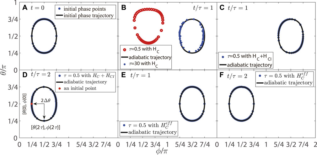
FIGURE 1. (A) Initial phase trajectory (solid line) and initial phase points (blue dots). (B) Final adiabatic trajectory (solid line) and final phase points driven by H_C when t/τ = 1, τ = .5 (red dot blanks) and τ = 30 (blue dots). (C) Final adiabatic trajectory (solid line) and final phase points driven by H_C + H_CI, when t/τ = 1 and τ = .5 (blue dots). (D) Final adiabatic trajectory (solid line) and final phase points driven by H_C + H_CI, when t/τ = 2 and τ = .5 (blue dots). (E) Final adiabatic trajectory (solid line) and final phase points driven by $H_I^{\mathit{eff}}$, when t/τ = 1 and τ = .5 (blue dots). (F) Final adiabatic trajectory (solid line) and final phase points driven by $H_I^{\mathit{eff}}$, when t/τ = 2 and τ = .5 (blue dots).

With the quantum−classical mapping method we introduced in the last section, we can derive a more explicit form of the TCD Hamiltonian $H_C^{\mathit{eff}}$ by averaging TQD Hamiltonian ${\widehat{H}}_{\mathit{eff}}$ Eq. 12. After a straightforward derivation, we have

$\begin{array}{ll}\hfill H_C^{\mathit{eff}}=& ⟨\psi |{\widehat{H}}_{\mathit{eff}}|\psi ⟩\hfill \\ \hfill =& \sum _n{E}_n|{\phi }_n{|}^2+i\hslash \sum _{n,m\ne n}{\phi }_m^{*}{\phi }_n⟨E_m|{\partial }_t{E}_n⟩\hfill \\ \hfill =& \sum _n{I}_n{\omega }_n-\sum _n{⟨p_n\left(\mathit{\theta },\mathit{I};t\right){\partial }_t{q}_n\left(\mathit{\theta },\mathit{I};t\right)⟩}_{\theta }+\frac{1}{2}\sum _n\left[p_n\left(\mathit{\theta },\mathit{I};t\right){\partial }_t{q}_n\left(\mathit{\theta },\mathit{I};t\right)-q_n\left(\mathit{\theta },\mathit{I};t\right){\partial }_t{p}_n\left(\mathit{\theta },\mathit{I};t\right)\right]\hfill \\ \hfill =& \sum _n{I}_n{\omega }_n-\sum _n{\partial }_t\left[p_n\left(\mathit{\theta },\mathit{I};t\right)q_n\left(\mathit{\theta },\mathit{I};t\right)\right],\hfill \end{array}(14)$

where ω_n = E_n/ℏ and the angular brackets ⟨⋯ ⟩ denote the averaging over all angle variables $\frac{1}{{(2\pi )}^N}{\mathrm{\Pi }}_k^N{\int }_0^{2\pi }d{\theta }_k$. Comparing Eq. 13 with Eq. 9, the terms canceling the non-adiabatic evolution and generating Hannay’s angle can be written as follows:

$\begin{array}{cc}\hfill \frac{\partial F}{\partial t}& =-\frac{1}{2}\sum _n\left[q_n\left(\mathit{\theta },\mathit{I};t\right){\partial }_t{p}_n\left(\mathit{\theta },\mathit{I};t\right)-p_n\left(\mathit{\theta },\mathit{I};t\right){\partial }_t{q}_n\left(\mathit{\theta },\mathit{I};t\right)\right],\hfill \\ \hfill A_H& =\sum _n{⟨p_n\left(\mathit{\theta },\mathit{I};t\right){\partial }_t{q}_n\left(\mathit{\theta },\mathit{I};t\right)⟩}_{\theta },\hfill \end{array}(15)$

respectively. Like the TQD, the choice of eigenfrequencies ω_n can be arbitrary and the geometric angles can be dropped for keeping the actions I conserved [10]. The simplest form of the Hamiltonian driving the canonical coordinates q and p with the conserved action I can be written as follows:

$H_I^{\mathit{eff}}=\frac{1}{2}\sum _n\left[p_n\left(\mathit{\theta },\mathit{I};t\right){\partial }_t{q}_n\left(\mathit{\theta },\mathit{I};t\right)-q_n\left(\mathit{\theta },\mathit{I};t\right){\partial }_t{p}_n\left(\mathit{\theta },\mathit{I};t\right)\right].(16)$

3.2 LR invariant-based scheme

A different approach to realize the quantum STA is based on the LR invariants [8, 58]. For the Hamiltonian $\widehat{H}(t)$, a time-dependent invariant can be determined by

$i\hslash \frac{\partial \widehat{I}\left(t\right)}{\partial t}+\left[\widehat{I}\left(t\right),\widehat{H}\left(t\right)\right]=0.(17)$

The eigenvalues λ_n of $\widehat{I}(t)$ remain constant over time, and the time-dependent eigenstates |λ_n(t)⟩ will accumulate an LR phase

${\mathrm{\Omega }}_n\left(t\right)=\frac{1}{\hslash }{\int }_0^t⟨{\lambda }_n\left(\tau \right)|i\hslash \frac{\partial }{\partial \tau }-H\left(\tau \right)|{\lambda }_n\left(\tau \right)⟩d\tau (18)$

via the dynamical evolution. By using the time-dependent unitary evolution operator

$U=\sum _n{e}^{i{\mathrm{\Omega }}_n\left(t\right)}|{\lambda }_n\left(t\right)\rangle \langle \lambda \left(0\right)|,(19)$

the Hamiltonian can be written as follows [8]:

${\widehat{H}}_d\equiv i\hslash \left({\partial }_{t}U\right)U^{†}=-\hslash \sum _n|{\lambda }_n\left(t\right)\rangle {\dot{\mathrm{\Omega }}}_n\langle {\lambda }_n\left(t\right)|+i\hslash \sum _n|{\partial }_t{\lambda }_n\left(t\right)\rangle \langle {\lambda }_n\left(t\right)|,(20)$

where the second term can be used to drive the eigenstates |λ_n(t)⟩ of $\widehat{I}(t)$ and generate the LR phase. Without loss of generality, the arbitrariness of choosing H_d can be fixed by the constrain $[\widehat{I}(0),\widehat{H}(0)]=0$ and $[\widehat{I}(t),\widehat{H}(t)]=0$ [8]. Invariant condition Eq. 17 can also be derived by comparing Eq. 20 with the original form of $\widehat{H}(t)$. Therefore, one can design an evolution path from the initial Hamiltonian $\widehat{H}(0)$ to the final one $\widehat{H}(T)$ along one of the eigenstates |λ_n(t)⟩ of $\widehat{I}(t)$ to achieve the STA.

For a classical system, we can also find similar classical time-dependent invariants that satisfy

${\dot{J}}_k=\frac{\partial J_k\left(t\right)}{\partial t}+\left\{J_k\left(t\right),H_C\left(\mathit{q},\mathit{p};t\right)\right\}=0.(21)$

By introducing a new pair of variables including the time-dependent invariants (ξ, J) (hereafter referred to as LR variables), we have the following canonical equations:

${\dot{J}}_k=-\frac{\partial G\left(\mathit{\alpha },t\right)}{\partial {\xi }_k}=0,{\dot{\xi }}_k=\frac{\partial G\left(\mathit{\alpha },t\right)}{\partial J_k},(22)$

where G(ξ, t) = H_C(ξ, J, t) + S(ξ, J, t) is the Hamiltonian after a classical transformation (q(t), p(t)) → (ξ(t), J) with the generating function S(q, I, t). Since J_k are invariants, the Hamiltonian G(ξ, t) does not contain the angle variables ξ_k. The changes of angles then can be rewritten as follows:

$\begin{array}{cc}\hfill \mathrm{\Delta }{\xi }_k=& {\int }_0^{T}dt\left(\frac{\partial {⟨H_C\left(\mathit{\xi },\mathit{J},t\right)⟩}_{\xi }}{\partial I_k}+\frac{\partial {⟨S\left(\mathit{\xi },\mathit{J},t\right)⟩}_{\xi }}{\partial I_k}\right),\hfill \\ \hfill =& {\int }_0^{T}dt\left(\frac{\partial {\bar{H}}_C\left(\mathit{J},t\right)}{\partial I_k}-\frac{\partial A_{LR}\left(\mathit{J},t\right)}{\partial I_k}\right)\hfill \end{array}(23)$

with ${\bar{H}}_C(\mathit{J},t)\equiv {⟨H_C(\mathit{\xi },\mathit{J},t)⟩}_{\xi }$ and $A_{LR}(\mathit{J},t)\equiv {\sum }_n{⟨p_n(\mathit{\xi },\mathit{J},t){\partial }_t{q}_n(\mathit{\xi },\mathit{J},t)⟩}_{\xi }$ which is similar to the dynamical part and geometrical part in the angle changes of the classical adiabatic evolution. The angular brackets ⟨⋯ ⟩_ξ denote an averaging over all LR angles ξ. Note that these LR variables are generally not action−angle variables of H_C. However, we can set {J_k(0), H_C(0)} = {J_k(T), H_C(T)} = 0; the LR action variables J_k can, thus, be chosen as action variables that are related to the eigenfrequencies at initial time t = 0 and final time t = T. Similar to the quantum STA based on LR invariants, we can also design an evolution path from H_C(0) to H_C(T) with the invariants J_k, in which the initial action variables of H are equal to those in the final time.

To determine the specific form of the classical LR invariant-based scheme, we define the probabilities amplitudes d_k of |Ψ⟩ = ∑_kd_k|λ_k⟩ on the LR basis {|λ_k⟩} as

$d_k=\sqrt{\frac{J_k}{\hslash }}{e}^{-i{\xi }_k},(24)$

using the quantum−classical mapping method. The canonical transformation (q, p) → (ξ, J) between position−momentum variables and LR variables can correspond to the quantum unitary transformation |λ_k(t)⟩ = ∑_nU_nk(t)|ψ_n⟩ between the adiabatic basis and the bare basis given as follows:

$\begin{array}{cc}\hfill & p_n\left(t\right)=\sum _k\sqrt{2J_k}\left\{\cos {\xi }_k\mathrm{I}\mathrm{m}\left[U_{nk}\left(t\right)\right]-\sin {\xi }_k\mathrm{R}\mathrm{e}\left[U_{nk}\left(t\right)\right]\right\},\hfill \\ \hfill & q_n\left(t\right)=\sum _k\sqrt{2J_k}\left\{\cos {\xi }_k\mathrm{R}\mathrm{e}\left[U_{nk}\left(t\right)\right]+\sin {\xi }_k\mathrm{I}\mathrm{m}\left[U_{nk}\left(t\right)\right]\right\}.\hfill \end{array}(25)$

Similar to the classical TQD scheme of the STA, the driving Hamiltonian should cancel the effect of the time-dependent transformation S and generate the angle Δξ_k. By Eqs 13–23, we have

$\begin{array}{l}{H}_d={\bar{H}}_C\left(\mathit{J},t\right)-A_{LR}\left(\mathit{J},t\right)-\frac{\partial S}{\partial t}\hfill \\ ={⟨H_C\left(\mathit{\xi },\mathit{J},t\right)⟩}_{\xi }-\sum _n\langle p_n\left(\mathit{\xi },\mathit{J},t\right){\partial }_t{q}_n{\left(\mathit{\xi },\mathit{J},t\right)\rangle }_{\xi }+\frac{1}{2}\sum _n\left[p_n\left(\mathit{\xi },\mathit{J};t\right){\partial }_t{q}_n\left(\mathit{\xi },\mathit{J};t\right)-q_n\left(\mathit{\xi },\mathit{J};t\right){\partial }_t{p}_n\left(\mathit{\xi },\mathit{J};t\right)\right],\hfill \end{array}(26)$

with

$\frac{\partial S}{\partial t}=-\frac{1}{2}\sum _n\left[p_n\left(\mathit{\xi },\mathit{J};t\right){\partial }_t{q}_n\left(\mathit{\xi },\mathit{J};t\right)-q_n\left(\mathit{\xi },\mathit{J};t\right){\partial }_t{p}_n\left(\mathit{\xi },\mathit{J};t\right)\right].(27)$

According to the quantum−classical mapping, this classical Hamiltonian of LR invariants method is just the mean value of the quantum LR, given as follows:

$H_d=⟨\psi |{\widehat{H}}_d|\psi ⟩.(28)$

Therefore, the form of LR variables can be determined by equating H_d and H_C, and the boundary conditions are as follows:

$\left\{J_k\left(0\right),H_C\left(0\right)\right\}=\left\{J_k\left(T\right),H_C\left(T\right)\right\}=0.(29)$

On the contrary, we can design the classical Hamiltonian H_d from the evolution of LR variables to realize the classical LR invariant-based scheme.

4 Spin-1/2 in a magnetic field

To illustrate our results, we consider the adiabatic evolution and STA scheme for a simple two-level quantum system, i.e., a spin-half particle with the magnetic moment μ in an external magnetic field B = B(sin α cos β, sin α sin β, cos α). Its Hamiltonian reads

$\widehat{H}=-\mu \widehat{\mathit{\sigma }}\cdot \mathit{B}=-\mu B\left(\begin{array}{cc}\hfill \cos \alpha \hfill & \hfill \sin \alpha e^{-i\beta }\hfill \\ \hfill \sin \alpha e^{i\beta }\hfill & \hfill -\cos \alpha \hfill \end{array}\right)=-\mu B\left[\cos \alpha \left(|+\rangle \langle +|-|-\rangle \langle -|\right)+\sin \alpha \left(e^{-i\beta }|+\rangle \langle -|+e^{i\beta }|-\rangle \langle +|\right)\right],(30)$

where $\widehat{\mathit{\sigma }}=({\widehat{\sigma }}_1,{\widehat{\sigma }}_2,{\widehat{\sigma }}_3)$ are Pauli matrices and |±⟩ are the two spin eigenstates.

4.1 Transitionless classical driving

As we introduced in the previous section, if the two spin eigenstates |±⟩ are chosen as the basis, the Hamiltonian in Eq. 30 can be mapped to the classical Hamiltonian of a coupled oscillator, given as follows:

$h\left(\mathit{p},\mathit{q};\mathit{B}\right)=-\frac{\mu B}{\hslash }\left[\frac{1}{2}\left(p_2^2+q_2^2-p_1^2-q_1^2\right)\cos \alpha +\left(p_1{q}_2-p_2{q}_1\right)\sin \alpha \sin \beta +\left(q_1{q}_2+p_1{p}_2\right)\sin \alpha \cos \beta \right],(31)$

with |ψ⟩ = ψ₁| − ⟩ + ψ₂| + ⟩ and ${\psi }_j=(q_j+i{p}_j)/\sqrt{2\hslash }$, (j = 1, 2). The canonical variables (q, p) satisfy the normalization condition [46], shown as follows:

$\sum _{j=1}^2\left(p_j^2+q_j^2\right)=2\hslash .(32)$

It is interesting to note that by defining a vector S = (S₁, S₂, S₃) with

$\left\{\begin{array}{c}{S}_1=⟨{\sigma }_1⟩=\left(q_1{q}_2+p_1{p}_2\right)/\hslash ,\hfill \\ S_2=⟨{\sigma }_2⟩=\left(p_1{q}_2-p_2{q}_1\right)/\hslash ,\hfill \\ S_3=⟨{\sigma }_3⟩=\left(p_2^2+q_2^2-p_1^2-q_1^2\right)/\left(2\hslash \right),\hfill \end{array}\right.(33)$

the Hamiltonian function can be written as follows:

$h\left(\mathit{S};\mathit{B}\right)=-\mu \mathit{S}\cdot \mathbf{B},(34)$

where the normalization condition of S is $S^2\equiv S_1^2+S_2^2+S_3^2=1$, and their Poisson bracket has a relation with the quantum commutator, shown as follows [45]:

$\left\{S_i,S_j\right\}=2{\epsilon }_{\mathit{ijk}}{S}_k/\hslash =\frac{1}{i\hslash }⟨\psi |\left[{\widehat{\sigma }}_i,{\widehat{\sigma }}_j\right]|\psi ⟩.(35)$

We now move to calculate Hannay’s angle. Since the Hamiltonian in Eq. 30 has two eigenstates,

$\begin{array}{cc}\hfill |E_1\rangle & =\cos \frac{\alpha }{2}|+\rangle +\sin \frac{\alpha }{2}{e}^{i\beta }|-\rangle ,\hfill \\ \hfill |E_2\rangle & =-\sin \frac{\alpha }{2}|+\rangle +\cos \frac{\alpha }{2}{e}^{i\beta }|-\rangle ,\hfill \end{array}(36)$

with eigenenergies −μB and μB, respectively. The canonical transformation (q, p) → (θ, I) and the mapped Hamiltonian function can be written as follows:

$\begin{array}{cc}\hfill q_1=& \sqrt{2I_1}\sin \frac{\alpha }{2}\cos \left(\beta -{\theta }_1\right)+\sqrt{2I_2}\cos \frac{\alpha }{2}\cos \left(\beta -{\theta }_2\right),\hfill \\ \hfill q_2=& \sqrt{2I_1}\cos \frac{\alpha }{2}\cos {\theta }_1-\sqrt{2I_2}\sin \frac{\alpha }{2}\cos {\theta }_2,\hfill \\ \hfill p_1=& \sqrt{2I_1}\sin \frac{\alpha }{2}\sin \left(\beta -{\theta }_1\right)+\sqrt{2I_2}\cos \frac{\alpha }{2}\sin \left(\beta -{\theta }_2\right),\hfill \\ \hfill p_2=& -\sqrt{2I_1}\cos \frac{\alpha }{2}\sin {\theta }_1+\sqrt{2I_2}\sin \frac{\alpha }{2}\sin {\theta }_2,\hfill \\ \bar{h}\left(\mathit{I};\mathit{B}\right)\hfill & =\mu B\left(I_2-I_1\right)/\hslash .\hfill \end{array}(37)$

We can calculate the forms of variable I by the following:

$\begin{array}{cc}\hfill I_1=& \frac{\hslash }{2}\left(1+\mathit{S}\cdot \mathit{b}\right),\hfill \\ \hfill I_2=& \frac{\hslash }{2}\left(1-\mathit{S}\cdot \mathit{b}\right)\hfill \end{array}(38)$

with q = (q₁, q₂), p = (p₁, p₂), θ = (θ₁, θ₂), I = (I₁, I₂), and b = B/B.

Therefore, we obtain the angle one-form by Eq. 9, given as follows:

$A_H=-\frac{1}{2}\left(1-\cos \alpha \right)\dot{\beta }{I}_1-\frac{1}{2}\left(1+\cos \alpha \right)\dot{\beta }{I}_2.(39)$

Hannay’s angles can, thus, be obtained by Eq. 10, given as follows:

$\begin{array}{cc}\hfill \mathrm{\Delta }{\theta }_1& =\oint \frac{1}{2}\left(1-\cos \alpha \right)\dot{\beta }dt,\hfill \\ \hfill \mathrm{\Delta }{\theta }_2& =\oint \frac{1}{2}\left(1+\cos \alpha \right)\dot{\beta }dt,\hfill \end{array}(40)$

which differ from the Berry phases in the original quantum Hamiltonian [58] only by a sign.

By Eq. 14, we have the following:

$\begin{array}{ll}\hfill H_I^{\mathit{eff}}=& \frac{1}{2}\left[\left(-p_1^2-q_1^2\right)\dot{\beta }+\left(p_1{q}_2-p_2{q}_1\right)\cos \beta \dot{\alpha }-\left(p_1{p}_2+q_1{q}_2\right)\sin \beta \dot{\alpha }\right]\hfill \\ \hfill =& \frac{\hslash }{2}\left[\left(S_3-1\right)\dot{\beta }+S_2\cos \beta \dot{\alpha }-S_1\sin \beta \dot{\alpha }\right],\hfill \end{array}(41)$

$\begin{array}{ll}\hfill A_H=& -\frac{1}{2}\left(1-\cos \alpha \right)I_1-\frac{1}{2}\left(1+\cos \alpha \right)I_2\hfill \\ \hfill =& -\frac{\hslash }{4}\left[\left(1-\cos \alpha \right)\left(1+\mathit{S}\cdot \mathit{b}\right)+\left(1+\cos \alpha \right)\left(1-\mathit{S}\cdot \mathit{b}\right)\right]\hfill \\ \hfill =& -\frac{\hslash }{2}\left(1-\cos \alpha \mathit{S}\cdot \mathit{b}\right).\hfill \end{array}(42)$

Therefore, we can get the TCD Hamiltonian function

$\begin{array}{ll}\hfill H_{CI}\left(\mathit{I};\mathit{\theta };\mathit{X}\right)=& \frac{\hslash }{2}\left[\left(S_3-1\right)\dot{\beta }+S_2\cos \beta \dot{\alpha }-S_1\sin \beta \dot{\alpha }\right]+\frac{\hslash }{2}\left(1-\cos \alpha \mathit{S}\cdot \mathit{b}\right)\dot{\beta }\hfill \\ \hfill =& \frac{\hslash }{2B^2}\mathit{S}\cdot \left(\mathit{B}\times \frac{\partial \mathit{B}}{\partial t}\right),\hfill \end{array}(43)$

which takes a similar form as the counter-adiabatic driving Hamiltonian for spin-1/2 system Eq. 30. This means that the TCD scheme can be treated like a classical version of the TQD scheme by representing coordinate−momentum variables by the classical “spin” defined by Eq. 33.

We illustrate the evolution of the states through their trajectories in the phase space. The evolution of the points on phase trajectories can be determined by the dynamic equation of classical “spin,” given as follows:

$\dot{S_i}=\left\{S_i,H_C\right\}=\frac{-2\mu B}{\hslash }{\epsilon }_{\mathit{ijk}}\left(b_j{S}_k-b_k{S}_j\right).(44)$

By defining θ = arccos S₂ and ϕ = arctan S₂/S₁, the dynamics of the original Hamiltonian H_C takes the following form:

$\begin{array}{cc}\hfill \dot{\theta }& =\frac{-2\mu B}{\hslash }\sin \alpha \sin \left(\beta -\varphi \right),\hfill \\ \hfill \dot{\varphi }& =\frac{-2\mu B}{\hslash }\left[\cos \alpha -\frac{\sin \alpha \cos \left(\beta -\varphi \right)}{\tan \theta }\right].\hfill \end{array}(45)$

The parameters of the magnetic field B are chosen as

$\begin{array}{cc}\hfill \alpha & =\frac{\pi }{2}-\frac{\pi }{4}\sin \frac{\pi t}{\tau },\beta =\pi -\frac{\pi }{2}\cos \frac{\pi t}{\tau },\hfill \\ \hfill \dot{\alpha }& =-\frac{{\pi }^2}{4\tau }\cos \frac{\pi t}{\tau },\dot{\beta }=\frac{{\pi }^2}{2\tau }\sin \frac{\pi t}{\tau },\hfill \end{array}(46)$

and μB/ℏ = −1.

As shown in Figure 1B, the evolution of the canonical coordinates p and q will keep the action variable I almost unchanged, and their trajectories in the phase space will follow adiabatic trajectories when the frequency is slow.

For the TCD Hamiltonian H_C + H_CI, the effective magnetic field changes into the following:

$\begin{array}{ll}\hfill {\mathit{B}}_{\mathit{eff}}=& \mathit{B}-\frac{\hslash }{2\mu }\left(\mathit{b}\times \dot{\mathit{b}}\right)\hfill \\ \hfill =& B\left\{\left[\sin \alpha \cos \beta +\frac{\hslash }{2\mu B}\left(\sin \beta \dot{\alpha }+\sin \alpha \cos \alpha \cos \beta \dot{\beta }\right)\right]\mathit{i}\right.\hfill \\ \hfill & +\left[\sin \alpha \sin \beta -\frac{\hslash }{2\mu B}\left(\cos \beta \dot{\alpha }-\sin \alpha \cos \alpha \sin \beta \dot{\beta }\right)\right]\mathit{j}\left.+\left(\cos \alpha -\frac{\hslash }{2\mu B}{\sin }^2\alpha \dot{\beta }\right)\mathit{k}\right\}.\hfill \end{array}(47)$

The dynamics of the TCD Hamiltonian can, thus, be written as follows:

$\begin{array}{cc}\hfill \dot{\theta }& =\cos \left(\beta -\varphi \right)\dot{\alpha }-\sin \alpha \sin \left(\beta -\varphi \right)\left(\frac{2\mu B}{\hslash }+\cos \alpha \dot{\beta }\right),\hfill \\ \hfill \dot{\varphi }& =-\frac{2\mu B}{\hslash }\cos \alpha +{\sin }^2\alpha \dot{\beta }+\frac{\sin \alpha \cos \left(\beta -\varphi \right)\left(2\mu B/\hslash +\cos \alpha \dot{\beta }\right)+\sin \left(\beta -\varphi \right)\dot{\alpha }}{\tan \theta }.\hfill \end{array}(48)$

To drive the eigenstates using H_C + H_CI, the evolution of the canonical coordinates p and q will keep action variables I unchanged, and their trajectories in the phase space will follow adiabatic trajectories no matter how fast the frequency is (see Figures 1C, D). By tracing the same phase points of the initial phase trajectory (see Figure 1A) and the final adiabatic trajectory, we can find that there is an angle of shift after an adiabatic evolution. Also, the angle of shift after a whole period is double that after half a period.

Moreover, for the simplest Hamiltonian Eq. 41 [dropping the constant term and the term generating the Hannay’s angle Eq. 42], the dynamics of the simplest Hamiltonian $H_I^{\mathit{eff}}$ is determined by the following:

$\begin{array}{cc}\hfill \dot{\theta }& =\cos \left(\beta -\varphi \right)\dot{\alpha },\hfill \\ \hfill \dot{\varphi }& =\dot{\beta }+\frac{\sin \left(\beta -\varphi \right)\dot{\alpha }}{\tan \theta }.\hfill \end{array}(49)$

It is easy to find that the adiabatic trajectories will remain unchanged after any period (see Figures 1E, F).

4.2 Classical LR invariant

In the approach of the LR invariant, the eigenstates of the LR invariant parallel to the eigenstates in Eq. 36 can be constructed as follows [8]:

$\begin{array}{cc}\hfill |{\lambda }_1\rangle & =\cos \frac{\eta }{2}|+\rangle +\sin \frac{\eta }{2}{e}^{i\delta }|-\rangle ,\hfill \\ \hfill |{\lambda }_2\rangle & =-\sin \frac{\eta }{2}|+\rangle +\cos \frac{\eta }{2}{e}^{i\delta }|-\rangle ,\hfill \end{array}(50)$

and the LR invariant can be expressed as follows:

$\widehat{I}\left(t\right)=\frac{\hslash }{2}{\mathrm{\Omega }}_0\left(\begin{array}{cc}\hfill \cos \eta \hfill & \hfill \sin \eta e^{-i\delta }\hfill \\ \hfill \sin \eta e^{i\delta }\hfill & \hfill -\cos \eta \hfill \end{array}\right).(51)$

In the classical expression of the adiabatic process, without loss of generality, the time-dependent classical invariants can be designed by classical spin Eq. 33 as follows:

$J_1=\frac{\hslash }{2}\left(1+\mathit{S}\cdot {\mathit{b}}^{\prime }\right),J_2=\frac{\hslash }{2}\left(1-\mathit{S}\cdot {\mathit{b}}^{\prime }\right).(52)$

where b′ = (sin η cos δ, sin η sin δ, cos η) is the scaling factor with the parameters (η, δ).

The canonical transformation between position−momentum variables (q, p) and LR variables (ξ, J) can be written as follows:

$\begin{array}{cc}\hfill q_1=& \sqrt{2J_1}\sin \frac{\eta }{2}\cos \left(\delta -{\xi }_1\right)+\sqrt{2J_2}\cos \frac{\eta }{2}\cos \left(\delta -{\xi }_2\right),\hfill \\ \hfill q_2=& \sqrt{2J_1}\cos \frac{\eta }{2}\cos {\xi }_1-\sqrt{2J_2}\sin \frac{\eta }{2}\cos {\xi }_2,\hfill \\ \hfill p_1=& \sqrt{2J_1}\sin \frac{\eta }{2}\sin \left(\delta -{\xi }_1\right)+\sqrt{2J_2}\cos \frac{\eta }{2}\sin \left(\delta -{\xi }_2\right),\hfill \\ \hfill p_2=& -\sqrt{2J_1}\cos \frac{\eta }{2}\sin {\xi }_1+\sqrt{2J_2}\sin \frac{\eta }{2}\sin {\xi }_2.\hfill \end{array}(53)$

After this canonical transformation, the Hamiltonian h(q, p; B) becomes

$\begin{array}{ll}\hfill G\left(\mathit{J};\mathit{B}\right)& ={\bar{H}}_C\left(\mathit{J};\mathit{B}\right)-A_{LR}\left(\mathit{J};\mathit{B}\right)\hfill \\ \hfill & =\frac{\mu }{\hslash }\mathit{B}\cdot {\mathit{b}}^{\prime }\left(J_2-J_1\right)+\frac{1}{2}\left[J_1\left(1-\cos \eta \right)+J_2\left(1+\cos \eta \right)\right]\dot{\delta }.\hfill \end{array}(54)$

We can calculate LR angles accumulated via the evolution process by Eq. 23, given as follows:

$\begin{array}{cc}\hfill \mathrm{\Delta }{\xi }_1& =\int dt\left[\frac{\mu }{\hslash }\mathit{B}\cdot {\mathit{b}}^{\prime }-\frac{1}{2}\left(1+\cos \eta \right)\dot{\delta }\right],\hfill \\ \hfill \mathrm{\Delta }{\xi }_2& =\int dt\left[-\frac{\mu }{\hslash }\mathit{B}\cdot {\mathit{b}}^{\prime }-\frac{1}{2}\left(1-\cos \eta \right)\dot{\delta }\right].\hfill \end{array}(55)$

According to Eq. 26, the driving Hamiltonian of the LR invariant-based scheme becomes

$\begin{array}{ll}\hfill H_d=& {\bar{H}}_C\left(\mathit{J},t\right)-A_{LR}\left(\mathit{J},t\right)-\frac{\partial S}{\partial t}\hfill \\ \hfill =& \frac{\mu }{\hslash }\mathit{B}\cdot \mathit{b}\left(J_2-J_1\right)+\left[\sin \left({\xi }_1-{\xi }_2\right)\dot{\eta }-\cos \left({\xi }_1-{\xi }_2\right)\sin \eta \dot{\delta }\right]\sqrt{J_1{J}_2},\hfill \\ \hfill =& S_3\left[-\mu \mathit{B}\cdot {\mathit{b}}^{\prime }\cos \eta +\frac{\hslash }{2}{\sin }^2\eta \dot{\delta }\right]+S_1\left[-\mu \mathit{B}\cdot {\mathit{b}}^{\prime }\sin \eta \cos \delta -\frac{\hslash }{2}\left(\sin \delta \dot{\eta }+\sin \eta \cos \eta \cos \delta \dot{\delta }\right)\right]\hfill \\ \hfill & +S_2\left[-\mu \mathit{B}\cdot {\mathit{b}}^{\prime }\sin \eta \sin \delta +\frac{\hslash }{2}\left(\cos \delta \dot{\eta }-\sin \eta \cos \eta \sin \delta \dot{\delta }\right)\right]\hfill \\ \hfill =& \mathit{S}\cdot {\mathit{B}}_d,\hfill \end{array}(56)$

where ${\mathit{B}}_d=(\mathit{B}\cdot {\mathit{b}}^{\prime }){\mathit{b}}^{\prime }-\frac{\hslash }{2\mu }{\mathit{b}}^{\prime }\times {\dot{\mathit{b}}}^{\prime }$. Comparing it with Eq. 34, the scaling factor b′ satisfies the following:

${\dot{\mathit{b}}}^{\prime }=\frac{2\mu }{\hslash }{\mathit{b}}^{\prime }\times \mathit{B}.(57)$

The system invariant boundary conditions in Eq. 29 become

${\dot{\mathit{b}}}^{\prime }\left(0\right)={\dot{\mathit{b}}}^{\prime }\left(T\right)=0,(58)$

and the driving magnetic field in the Hamiltonian H can be chosen as

$\mathit{B}=-\frac{\hslash }{2\mu }{\mathit{b}}^{\prime }\times {\dot{\mathit{b}}}^{\prime }(59)$

to realize the evolution from initial energy eigenstates |λ_n(0)⟩ to final energy eigenstates |λ_n(T)⟩.

By equating Hamiltonian H_d Eq. 56 and ${\bar{H}}_C(\mathit{J},t)$, we can calculate these two pairs of parameters satisfying the following equation:

$\begin{array}{cc}\hfill \dot{\delta }& =\frac{-2\mu B}{\hslash }\left[\cos \alpha +\sin \alpha \frac{\cos \eta }{\sin \eta }\cos \left(\beta -\delta \right)\right],\hfill \\ \hfill \dot{\eta }& =\frac{-2\mu B}{\hslash }\sin \alpha \sin \left(\beta -\delta \right).\hfill \end{array}(60)$

In particular, there is still arbitrariness in the choice of parameters η and δ. To illustrate the adiabatic evolution driven by Eq. 56, we make the invariants of the initial and final moments satisfy the boundary conditions and Eq. 60. For example, to transfer the state from the first oscillator with canonical variables q₁ and p₁ to the second oscillator with canonical variables q₂ and p₂, we can set $\dot{\eta }(0)=0$, η(0) = 0, and η(T) = π to satisfy the boundary conditions and chose a different scheme for δ.

To illustrate this result, we choose two different configurations of time-dependent parameters as shown in Figure 2. The first set of parameters

$\begin{array}{cc}\hfill \eta & =\frac{\pi }{2}+\frac{\pi }{2}\cos \frac{\pi t}{\tau },\hfill \\ \hfill \delta & =-\frac{\pi }{2}+\sin \frac{\pi t}{\tau }\hfill \end{array}(61)$

in Figure 2A which implements the adiabatic invariance of action variables can reproduce the evolution manipulated by the TQD Hamiltonian Eq. 43 as shown in Figure 2B. The action variables J_i exactly follow the adiabatic trajectories. The evolution of the phase trajectory is just like that in Figures 1A, E driven by $H_C^{\mathit{eff}}$. Similar to the fact that the TQD can be seen as one of the schemes for the inverse engineering based on the quantum LR invariant [59], the TCD which keeps the evolution exactly on the adiabatic trajectories in phase space of the classical Hamiltonian can be seen as one of the schemes for inverse engineering based on the classical LR invariant, which only needs the initial and final trajectories in the phase space matching adiabatic trajectories in the phase space of the classical Hamiltonian. Therefore, we can also design the classical Hamiltonian by different parameters to realize the classical LR invariant scheme. For example, the parameters

$\begin{array}{cc}\hfill \eta & =\pi -3\pi t^2+2\pi t^3,\hfill \\ \hfill \delta & =-\frac{\pi }{2}+\frac{\pi }{2}t-\frac{5\pi }{2}{t}^2+4\pi t^3-2\pi t^4\hfill \end{array}(62)$

in Figure 2C can also realize the state transfer between the two oscillators with a nearly unchanged δ. Thus, the optional form of the parameters to implement the adiabatic invariance is not unique. These results can be perfectly related to the LR invariant method for the spin-1/2 system [59].

FIGURE 2

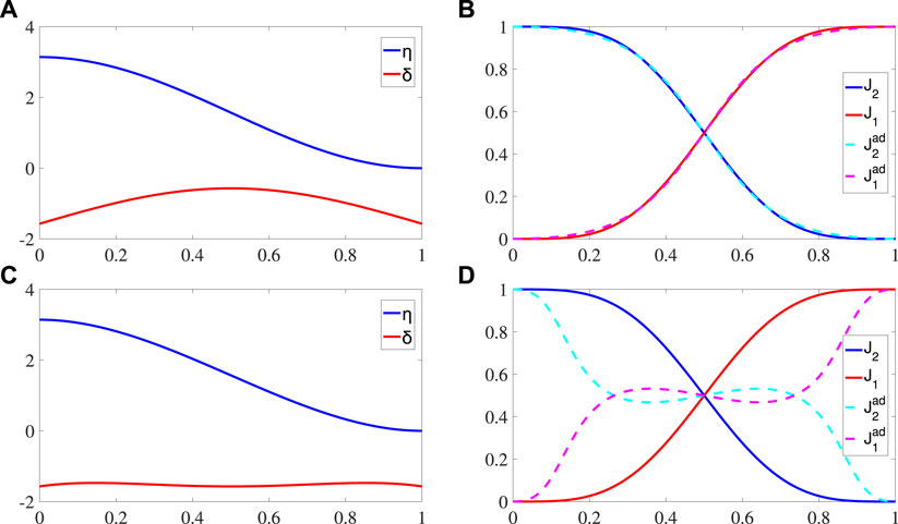
FIGURE 2. (A−C) Evolution of the parameters η (solid blue line) and δ (solid red line). (B−D) Time evolution of the action variables J₁ (solid red line), J₂ (solid blue line) driven by H_d, and adiabatic approximate invariants $J_1^{ad}$ (dashed red line) and $J_2^{ad}$ (dashed blue line) when t/τ = 1 and τ = .5.

5 Conclusion

To sum up, we use the quantum−classical mapping method to simulate the two schemes of the STA, i.e., the TQD and quantum LR invariant method, by the classical system consisting of coupled oscillators. On one hand, for the TQD, which implements the STA by finding an additional Hamiltonian to drive the system, we derived the explicit form of an additional driving Hamiltonian to keep the evolution of adiabatic phase trajectories and acquire the Hannay’s phase. This TCD method can perfectly simulate and match the TQD method. On the other hand, the Lewis−Riesenfeld invariant method, which keeps the energy eigenstates from a specified initial to the final configuration, can also be simulated by manipulating the configurations of classical coupled oscillators. Both of the approaches can accelerate the adiabatic process effectively under different circumstances and matches the quantum methods of the STA. These results prove that the protocol of the quantum−classical mapping can be used to generalize quantum schemes of the STA into the classical system. By this simulation, our theory could be expected to find applications of the STA for classical systems.

Data availability statement

The original contributions presented in the study are included in the article/Supplementary Material; further inquiries can be directed to the corresponding authors.

Author contributions

HL and HS initiated the idea. YL and HL wrote the main manuscript text. YL and YZ performed the calculations.

Funding

This work was supported by the National Natural Science Foundation of China (Contact Nos. 11875103 and 12147206).

Conflict of interest

The authors declare that the research was conducted in the absence of any commercial or financial relationships that could be construed as a potential conflict of interest.

Publisher’s note

All claims expressed in this article are solely those of the authors and do not necessarily represent those of their affiliated organizations, or those of the publisher, the editors, and the reviewers. Any product that may be evaluated in this article, or claim that may be made by its manufacturer, is not guaranteed or endorsed by the publisher.

References

1. Li YC, Chen X. Shortcut to adiabatic population transfer in quantum three-level systems: Effective two-level problems and feasible counterdiabatic driving. Phys Rev A (2016) 94:063411. doi:10.1103/PhysRevA.94.063411

CrossRef Full Text | Google Scholar

2. Král P, Thanopulos I, Shapiro M. Colloquium: Coherently controlled adiabatic passage. Rev Mod Phys (2007) 79:53–77. doi:10.1103/RevModPhys.79.53

CrossRef Full Text | Google Scholar

3. Saffman M, Walker TG, Mølmer K. Quantum information with rydberg atoms. Rev Mod Phys (2010) 82:2313–63. doi:10.1103/RevModPhys.82.2313

CrossRef Full Text | Google Scholar

4. Vitanov NV, Rangelov AA, Shore BW, Bergmann K. Stimulated Raman adiabatic passage in physics, chemistry, and beyond. Rev Mod Phys (2017) 89:015006. doi:10.1103/RevModPhys.89.015006

CrossRef Full Text | Google Scholar

5. Chen X, Ruschhaupt A, Schmidt S, del Campo A, Guéry-Odelin D, Muga JG. Fast optimal frictionless atom cooling in harmonic traps: Shortcut to adiabaticity. Phys Rev Lett (2010) 104:063002. doi:10.1103/PhysRevLett.104.063002

PubMed Abstract | CrossRef Full Text | Google Scholar

6. Longuet-Higgins HC, Öpik U, Pryce MHL, Sack RA. Studies of the jahn-teller effect. ii. the dynamical problem. Proc R Soc A: Math Phys Eng Sci (1958) 244 (1236):1–16. doi:10.1098/rspa.1958.0022

CrossRef Full Text | Google Scholar

7. Pancharatnam S. Generalized theory of interference, and its applications. Proc Indian Acad Sci A (1956) 44:247–62. doi:10.1007/BF03046050

CrossRef Full Text | Google Scholar

8. Chen X, Torrontegui E, Muga JG. Lewis-Riesenfeld invariants and transitionless quantum driving. Phys Rev A (2011) 83:062116. doi:10.1103/PhysRevA.83.062116

CrossRef Full Text | Google Scholar

9. Rezek Y, Kosloff R. Irreversible performance of a quantum harmonic heat engine. New J Phys (2006) 8:83. doi:10.1088/1367-2630/8/5/083

CrossRef Full Text | Google Scholar

10. Berry MV. Transitionless quantum driving. J Phys A: Math Theor (2009) 42:365303. doi:10.1088/1751-8113/42/36/365303

CrossRef Full Text | Google Scholar

11. Ban Y, Chen X, Sherman EY, Muga JG. Fast and robust spin manipulation in a quantum dot by electric fields. Phys Rev Lett (2012) 109:206602. doi:10.1103/PhysRevLett.109.206602

PubMed Abstract | CrossRef Full Text | Google Scholar

12. Ban Y, Jiang LX, Li YC, Wang LJ, Chen X. Fast creation and transfer of coherence in triple quantum dots by using shortcuts to adiabaticity. Opt Express (2018) 26:31137–49. doi:10.1364/OE.26.031137

PubMed Abstract | CrossRef Full Text | Google Scholar

13. Chen X, Jiang RL, Li J, Ban Y, Sherman EY. Inverse engineering for fast transport and spin control of spin-orbit-coupled bose-einstein condensates in moving harmonic traps. Phys Rev A (2018) 97:013631. doi:10.1103/PhysRevA.97.013631

CrossRef Full Text | Google Scholar

14. Zhang J, Shim JH, Niemeyer I, Taniguchi T, Teraji T, Abe H, et al. Experimental implementation of assisted quantum adiabatic passage in a single spin. Phys Rev Lett (2013) 110:240501. doi:10.1103/PhysRevLett.110.240501

PubMed Abstract | CrossRef Full Text | Google Scholar

15. del Campo A. Shortcuts to adiabaticity by counterdiabatic driving. Phys Rev Lett (2013) 111:100502. doi:10.1103/PhysRevLett.111.100502

PubMed Abstract | CrossRef Full Text | Google Scholar

16. del Campo A. Frictionless quantum quenches in ultracold gases: A quantum-dynamical microscope. Phys Rev A (2011) 84:031606. doi:10.1103/PhysRevA.84.031606

CrossRef Full Text | Google Scholar

17. Chen YH, Shi ZC, Song J, Xia Y. Invariant-based inverse engineering for fluctuation transfer between membranes in an optomechanical cavity system. Phys Rev A (2018) 97:023841. doi:10.1103/PhysRevA.97.023841

CrossRef Full Text | Google Scholar

18. Lu M, Xia Y, Shen LT, Song J, An NB. Shortcuts to adiabatic passage for population transfer and maximum entanglement creation between two atoms in a cavity. Phys Rev A (2014) 89:012326. doi:10.1103/PhysRevA.89.012326

CrossRef Full Text | Google Scholar

19. Chen YH, Xia Y, Wu QC, Huang BH, Song J. Method for constructing shortcuts to adiabaticity by a substitute of counterdiabatic driving terms. Phys Rev A (2016) 93:052109. doi:10.1103/PhysRevA.93.052109

CrossRef Full Text | Google Scholar

20. Deffner S, Jarzynski C, del Campo A. Classical and quantum shortcuts to adiabaticity for scale-invariant driving. Phys Rev X (2014) 4:021013. doi:10.1103/PhysRevX.4.021013

CrossRef Full Text | Google Scholar

21. Chen X, Lizuain I, Ruschhaupt A, Guéry-Odelin D, Muga JG. Shortcut to adiabatic passage in two- and three-level atoms. Phys Rev Lett (2010) 105:123003. doi:10.1103/PhysRevLett.105.123003

PubMed Abstract | CrossRef Full Text | Google Scholar

22. Jarzynski C, Deffner S, Patra A, Subaşı Y. Fast forward to the classical adiabatic invariant. Phys Rev E (2017) 95:032122 (3). doi:10.1103/PhysRevE.95.032122

PubMed Abstract | CrossRef Full Text | Google Scholar

23. Okuyama M, Takahashi K. From classical nonlinear integrable systems to quantum shortcuts to adiabaticity. Phys Rev Lett (2016) 117:070401. doi:10.1103/PhysRevLett.117.070401

PubMed Abstract | CrossRef Full Text | Google Scholar

24. Jarzynski C. Generating shortcuts to adiabaticity in quantum and classical dynamics. Phys Rev A (2013) 88:040101. doi:10.1103/PhysRevA.88.040101

CrossRef Full Text | Google Scholar

25. Deng J, Wang Q, Liu Z, Hänggi P, Gong J. Boosting work characteristics and overall heat-engine performance via shortcuts to adiabaticity: Quantum and classical systems. Phys Rev E (2013) 88:062122. doi:10.1103/PhysRevE.88.062122

PubMed Abstract | CrossRef Full Text | Google Scholar

26. Xiao G, Gong J. Suppression of work fluctuations by optimal control: An approach based on jarzynski’s equality. Phys Rev E (2014) 90:052132. doi:10.1103/PhysRevE.90.052132

PubMed Abstract | CrossRef Full Text | Google Scholar

27. Olavo L. Quantum mechanics as a classical theory; 2, relativistic theory. Tech. Rep. quant-ph/9503021 (1995).

Google Scholar

28. Arnold VI. Mathematical methods of classical mechanics. In: Graduate texts in mathematics, Vol. 60. New York, NY: Springer-Verlag (1978). doi:10.1007/978-1-4757-1693-1

CrossRef Full Text | Google Scholar

29. Peres A, Terno DR. Hybrid classical-quantum dynamics. Phys Rev A (2001) 63:022101. doi:10.1103/PhysRevA.63.022101

CrossRef Full Text | Google Scholar

30. Elze HT. Linear dynamics of quantum-classical hybrids. Phys Rev A (2012) 85:052109. doi:10.1103/PhysRevA.85.052109

CrossRef Full Text | Google Scholar

31. Gil V, Salcedo LL. Canonical bracket in quantum-classical hybrid systems. Phys Rev A (2017) 95:012137. doi:10.1103/PhysRevA.95.012137

CrossRef Full Text | Google Scholar

32. Kantner M, Mittnenzweig M, Koprucki T. Hybrid quantum-classical modeling of quantum dot devices. Phys Rev B (2017) 96:205301. doi:10.1103/PhysRevB.96.205301

CrossRef Full Text | Google Scholar

33. Briggs JS, Eisfeld A. Equivalence of quantum and classical coherence in electronic energy transfer. Phys Rev E (2011) 83:051911. doi:10.1103/PhysRevE.83.051911

PubMed Abstract | CrossRef Full Text | Google Scholar

34. Briggs JS, Eisfeld A. Coherent quantum states from classical oscillator amplitudes. Phys Rev A (2012) 85:052111. doi:10.1103/PhysRevA.85.052111

CrossRef Full Text | Google Scholar

35. Briggs JS, Eisfeld A. Quantum dynamics simulation with classical oscillators. Phys Rev A (2013) 88:062104. doi:10.1103/PhysRevA.88.062104

CrossRef Full Text | Google Scholar

36. Briggs JS. Equivalent emergence of time dependence in classical and quantum mechanics. Phys Rev A (2015) 91:052119. doi:10.1103/PhysRevA.91.052119

CrossRef Full Text | Google Scholar

37. Radonjić M, Prvanović S, Burić N. System of classical nonlinear oscillators as a coarse-grained quantum system. Phys Rev A (2011) 84:022103. doi:10.1103/PhysRevA.84.022103

CrossRef Full Text | Google Scholar

38. Radonjić M, Prvanović S, Burić N. Hybrid quantum-classical models as constrained quantum systems. Phys Rev A (2012) 85:064101. doi:10.1103/PhysRevA.85.064101

CrossRef Full Text | Google Scholar

39. Radonjić M, Prvanović S, Burić N. Emergence of classical behavior from the quantum spin. Phys Rev A (2012) 85:022117. doi:10.1103/PhysRevA.85.022117

CrossRef Full Text | Google Scholar

40. Burić N, Popović DB, Radonjić M, Prvanović S. Orbits of hybrid systems as qualitative indicators of quantum dynamics. Phys Lett A (2014) 378 (16):1081–1084. doi:10.1016/j.physleta.2014.02.037

CrossRef Full Text | Google Scholar

41. Arsenović D, Burić N, Popović DB, Radonjić M, Prvanović S. Positive-operator-valued measures in the Hamiltonian formulation of quantum mechanics. Phys Rev A (2015) 91:062114. doi:10.1103/PhysRevA.91.062114

CrossRef Full Text | Google Scholar

42. Polchinski J. Weinberg’s nonlinear quantum mechanics and the einstein-podolsky-rosen paradox. Phys Rev Lett (1991) 66:397–400. doi:10.1103/PhysRevLett.66.397

PubMed Abstract | CrossRef Full Text | Google Scholar

43. Chruściński D, Jamiołkowski A. Geometric phases in classical and quantum mechanics. In: Progress in mathematical physics, Vol. 36. Boston, MA: Springer Science and Business Media (2012). doi:10.1007/978-0-8176-8176-0

CrossRef Full Text | Google Scholar

44. Zhang Q, Wu B. General approach to quantum-classical hybrid systems and geometric forces. Phys Rev Lett (2006) 97:190401. doi:10.1103/PhysRevLett.97.190401

PubMed Abstract | CrossRef Full Text | Google Scholar

45. Heslot A. Quantum mechanics as a classical theory. Phys Rev D (1985) 31:1341–8. doi:10.1103/PhysRevD.31.1341

PubMed Abstract | CrossRef Full Text | Google Scholar

46. Weinberg S. Testing quantum mechanics. Ann Phys (N Y) (1989) 194:336–86. doi:10.1016/0003-4916(89)90276-5

CrossRef Full Text | Google Scholar

47. Weinberg S. Precision tests of quantum mechanics. Phys Rev Lett (1989) 62:485–8. doi:10.1103/PhysRevLett.62.485

PubMed Abstract | CrossRef Full Text | Google Scholar

48. Wu B, Liu J, Niu Q. Geometric phase for adiabatic evolutions of general quantum states. Phys Rev Lett (2005) 94:140402. doi:10.1103/PhysRevLett.94.140402

PubMed Abstract | CrossRef Full Text | Google Scholar

49. Zhang Q, Wu B. General approach to quantum-classical hybrid systems and geometric forces. Phys Rev Lett (2006) 97:190401. doi:10.1103/PhysRevLett.97.190401

PubMed Abstract | CrossRef Full Text | Google Scholar

50. Stone M. Born-oppenheimer approximation and the origin of wess-zumino terms: Some quantum-mechanical examples. Phys Rev D (1986) 33:1191–4. doi:10.1103/PhysRevD.33.1191

PubMed Abstract | CrossRef Full Text | Google Scholar

51. Gozzi E, Thacker WD. Classical adiabatic holonomy and its canonical structure. Phys Rev D (1987) 35:2398–406. doi:10.1103/physrevd.35.2398

PubMed Abstract | CrossRef Full Text | Google Scholar

52. Liu HD, Wu SL, Yi XX. Berry phase and hannay’s angle in a quantum-classical hybrid system. Phys Rev A (2011) 83:062101. doi:10.1103/PhysRevA.83.062101

CrossRef Full Text | Google Scholar

53. Heslot A. Quantum mechanics as a classical theory. Phys Rev D (1985) 31:1341–8. doi:10.1103/PhysRevD.31.1341

PubMed Abstract | CrossRef Full Text | Google Scholar

54. Strocchi F. Complex coordinates and quantum mechanics. Rev Mod Phys (1966) 38:36–40. doi:10.1103/RevModPhys.38.36

CrossRef Full Text | Google Scholar

55. Dirac PAM, Bohr NHD. The quantum theory of the emission and absorption of radiation. Proc R Soc Lond A (1927) 114:243–65. doi:10.1098/rspa.1927.0039

CrossRef Full Text | Google Scholar

56. Berry MV. Quantal phase factors accompanying adiabatic changes. Proc R Soc Lond A (1984) 392 (1802):45–57. The Royal Society London. doi:10.1098/rspa.1927.0039

CrossRef Full Text | Google Scholar

57. Berry MV. Classical adiabatic angles and quantal adiabatic phase. J Phys A: Math Gen (1985) 18:15–27. doi:10.1088/0305-4470/18/1/012

CrossRef Full Text | Google Scholar

58. Lewis HR, Riesenfeld W. An exact quantum theory of the time-dependent harmonic oscillator and of a charged particle in a time-dependent electromagnetic field. J Math Phys (1969) 10:1458–73. doi:10.1063/1.1664991

CrossRef Full Text | Google Scholar

59. Chen X, Torrontegui E, Muga JG. Lewis-riesenfeld invariants and transitionless quantum driving. Phys Rev A (2011) 83:062116. doi:10.1103/PhysRevA.83.062116

CrossRef Full Text | Google Scholar

Appendix: Derivation of the Schrödinger equation in the canonical form

The dynamical evolution of the N-level quantum system governed by the Hamiltonian $\widehat{H}(t)$ can be described by the following Schrödinger equation:

$i\hslash {\partial }_t|\mathrm{\Psi }\rangle =\widehat{H}\left(t\right)|\mathrm{\Psi }\rangle ,(63)$

which can be expanded by the quantum state |Ψ⟩ = ∑ψ_n(t)|ψ_n⟩ as follows:

$i\hslash {\partial }_t\left(\sum _n{\psi }_n\left(t\right)|{\psi }_n\rangle \right)=\widehat{H}\left(t\right)|\mathrm{\Psi }\rangle ,(64)$

with the probability amplitudes ψ_n on the bare basis {|ψ_n⟩}. Since {|ψ_n⟩} is a time-independent bare basis, Eq. 64 becomes

$i\hslash d_t{\psi }_n\left(t\right)|{\psi }_n\rangle =\widehat{H}\left(t\right)|\mathrm{\Psi }\rangle .(65)$

Multiplying Eq. 65 by ⟨ψ_m|, we have the following:

$i\hslash d_t{\psi }_m\left(t\right)=⟨{\psi }_m|\widehat{H}\left(t\right)|\mathrm{\Psi }⟩,(66)$

with $H_C(\mathit{\psi },{\mathit{\psi }}^{*},t)=⟨\mathrm{\Psi }|\widehat{H}(t)|\mathrm{\Psi }⟩={\sum }_m{\psi }_m^{*}⟨m|\widehat{H}(t)|\mathrm{\Psi }⟩$. Therefore, the Schrödinger equation in the canonical form can be written as follows:

$i\hslash \frac{d{\psi }_m\left(t\right)}{dt}=\frac{\partial H_C}{\partial {\psi }_m^{*}},(67)$

which is just the same as Eq. 1.