 Xiuyun Chen1,2
 Yanming Xu
 Wenqiang Ma
- 1School of Architecture and Civil Engineering, Huanghuai University, Zhumadian, China
- 2Henan International Joint Laboratory of Structural Mechanics and Computational Simulation, Huanghuai University, Zhumadian, China
- 3College of Architecture and Civil Engineering, Xinyang Normal University, Xinyang, China
In many engineering challenges, the whole interaction between the structural domain and the acoustic domain must be taken into account, particularly for the acoustic analysis of thin structures submerged in water. The fast multipole boundary element approach is used in this work to simulate the external acoustic domain and the finite element method is used to describe the structural components. To improve coupling analysis accuracy, discontinuous higher-order boundary components are created for the acoustic domain. The isogeometric boundary element method (IGABEM) discretizes unknown physical fields by using CAD spline functions as basis functions. IGABEM is inherently compatible with CAD and can perform numerical analysis on CAD models without having to go through the time-consuming meshing process required by traditional FEM/BEM and volume parameterization in isogeometric finite element methods. IGABEM’s power in tackling infinite domain issues and combining CAD and numerical analysis is fully used when it is applied to structural form optimization of three-dimensional external acoustic problems. The structural-acoustic design and optimization procedures benefit from the use of structural-acoustic design sensitivity analysis because it may provide information on how design factors affect radiated acoustic performance. This paper provides adjoint operator-based equations for sound power sensitivity on structural surfaces and direct differentiation-based equations for sound power sensitivity on arbitrary closed surfaces surrounding the radiator. Numerical illustrations are provided to show the precision and viability of the suggested approach.
1 Introduction
A typical issue in underwater acoustics is the analysis of the acoustic radiation or scattering from elastic structures in fluid. Only for basic geometric structures with simple boundary conditions are analytical solutions to structural-acoustic interaction issues accessible [1]. There are still no analytical answers to real-world issues with complex geometries. Therefore, effective numerical techniques must be created.
Due to its high adaptability and suitability for complex real-world model challenges, the finite element method (FEM) is frequently employed to simulate the structural components in these issues [2]. To avoid meshing the commonly infinite or semi-infinite acoustic domain, the sound field is modeled using the boundary element method (BEM) [3]. Researchers have focused a lot of their attention on the FEM/BEM coupling techniques [4]; [5]; [6]; [7]; [8]; [9,10]; [11]; [12], where FEM is used to discretize the structure’s components and BEM is utilized to represent the acoustic area. BEM frequently employs continuous linear or quadratic components. Discontinuous elements have been researched as an alternative to them, exhibiting a high level of precision [13]; [14]. When a hypersingular integral is discretized, discontinuous boundary elements are typically used because C1-continuity of the surface at the collocation point is necessary in such situation. Applications can be found in fracture analysis [15] and the Navier-Stokes equation solution [16]. When collocation points are situated at the zeros of orthogonal functions for the standard interval, superconvergence for error dependency on the size of discontinuous border elements has been examined by [17]; [14] presents the error dependency of the frequency, element size, and node placement on discontinuous elements. This study discovered that discontinuous border elements outperform continuous components in terms of performance. In-depth research has also been done on how well discontinuous boundary elements perform in acoustic analyses of rigid structures. [18] Discussed how discontinuous boundary elements combined with FEM perform when the interaction between the structure and the sound field is taken into consideration.
Conventional BEM has the well-known drawback of generating a dense and asymmetrical coefficient matrix, which necessitates O(N3) arithmetic operations to directly solve the system of equations, such as by applying the Gauss elimination technique. The integral problem has been solved more quickly using the fast multipole method (FMM) [19]; [20]; [21]; [22]. Iterative solvers have proven to be effective in solving complex practical issues [23]; [24]. Therefore, large-scale acoustic-structure interaction issues may be successfully solved using the coupling technique based on FEM and fast multipole BEM (FMBEM) [7]; [8]. The diagonal form of the FMM and the original FMM are both utilized to solve the Helmholtz problem. Outside the ranges of their favored frequencies, both kinds fail in some way. However, the aforementioned issues can be resolved by the wideband FMM created by fusing the original FMM and the diagonal form FMM [25]; [26]. The main use of FMM is for discretization-based numerical analysis using constant boundary elements. Due to the difficulty of the computation process, there are not many articles that employ the FMM for numerical analysis based on discontinuous high-order boundary element discretization [18]. In this research, FMM is employed to speed up the solution of the integral equation using discontinuous boundary elements. Finally, the large-scale acoustic-structure interaction issues are solved using the coupling algorithm FEM/discontinuous wideband FMBEM.
Both conventional FEM and BEM with Lagrange polynomial basis functions rely on polygonal meshes, which leads to time-consuming preprocessing steps, geometric inaccuracies, and poor field variable continuity [27]. The [28] notion of isogeometric analysis (IGA) allows for the resolution of these problems. The core of IGA is to discretize the unknown physical fields while solving partial differential equations by using the same basis functions as those in computer-aided design (CAD) to describe the domain geometry. Geometric accuracy, adjustable order elevation and k-refinement, high order continuous fields, etc. are some benefits of IGA. Although IGA was first created in the context of finite element methods (IGAFEM), there are some situations when it is preferable to combine IGA with boundary element methods (IGABEM) [10, 29]; [30]; [31]; [32, 33]. Several benefits come with IGABEM:
• it can use CAD data right away without the need for volume parameterization from geometric surfaces [34, 35], since both of them are boundary-represented [36]; [37]; [38];
• it inherits the benefits of traditional BEM for addressing problems in infinite domains [39]; [40–42];
• IGABEM is perfect for free boundary problems like crack growth since no volume parameterization is required [43, 44].
As for the singularity problems, singularities and shifting borders are well handled by IGA [43, 44]. Specialized integration methods have been developed to tackle the weakly singular and hypersingular integrals that arise in IGABEM [41].
Acoustic design sensitivity analysis is crucial to the acoustic design and optimization processes because it may provide information about the impact of geometric modifications on the acoustic performance of structures [45]. An overview of recent advancements in structural-acoustic optimization for passive noise suppression was provided by [6]. Gradient-based optimization takes a long time to do a sound power sensitivity analysis for problems involving acoustic-structure interaction. The global finite difference method (FDM) is frequently used in structural-acoustic optimization because it is simple to employ, according to [46], [47], and [48]. However, FDM performs poorly, especially when several design elements are taken into account at once. The distinction between semi-analytic and analytical sensitivity studies has been made in addition to global finite differences. These classifications have been debated in many studies [49]; [6,50]. Global finite differences are significantly less accurate than analytical and semi-analytical sensitivity studies. Additionally, the former are less expensive computationally than the latter. In [51], coupled structural acoustic issues were addressed using an analytical sensitivity analysis, which has recently emerged as the direct differentiation approach. Using the adjoint operator technique, which has been used to solve structural acoustic problems, allows for still further acceleration in calculation time, particularly for issues with several design variables [52]; [53].
With regard to several design variables, this work constructs equations for sound power sensitivity. To eliminate geometric errors, the fundamental formulations of IGABEM discretization are introduced for acoustic analysis. Directly differentiating the coupled boundary element equation with respect to design variables yields the derivative formulation of the vectors of nodal displacement and sound pressure on the interaction surface with respect to design variables. The coupled boundary element equation is created by fusing the structural equation into the acoustic equation. Utilizing adjoint operators and direct differentiation, respectively, we derive the derivative formulation of the radiated sound power on the structural surface and the derivative formulation of the radiated sound power on any arbitrary closed surface around the radiator. The appropriate formula needed to compute the derivative of the radiated sound power for various design variables are discussed in detail. The FEM/FMBEM coupling system is used to determine the sound power sensitivity. It is shown with numerical examples how accurate and reliable the current method is.
2 Structural-acoustic analysis
2.1 Subdivision surfaces
Since its introduction in the 1970s, subdivision surfaces have been extensively utilized in computer animation and graphics [54]. Additionally, they are accessible in the majority of industrial CAD solid modeling programs (e.g., CATIA, Creo). Subdivision surfaces are often seen in computer graphics literature as a method for repeatedly smoothing and refining a control mesh in order to generate smooth limit surfaces. They may also be seen from the perspective of finite and boundary element analysis as the generalization of splines to arbitrarily connected meshes.
The concept of subdivision schemes is to create a smooth surface out of a rough polygon mesh. Subdivision refinement systems, which may be categorized as interpolating or approximation schemes, create a smooth surface by a limited process of repetitive refinement beginning with an initial control mesh. All control meshes produced during subdivision refinement describe the exact same spline surface since the subdivision surfaces inherit the refinability attribute from the splines.
In this research, the structural-acoustic coupling analysis is conducted using a Loop subdivision technique [42].
2.2 Acoustic-structure interaction using finite element method/boundary element method
The BEM and FEM are used to simulate the fluid and structural subdomains, respectively. The discretized boundary integral formulation of the fluid solution to the Helmholtz problem is given by [55], as shown in Equation 1:
where
H and G are the frequency-dependent BEM influencing matrices,
p is the vector containing the nodal values for pressure,
q is the vector of normal derivatives of p,
pi is the incident wave’s nodal pressure.
The continuous linear and quadratic element technique is often used, and alternatives to discontinuous elements with good accuracy have already been examined [14]. Discontinuous boundary elements outperform continuous boundary elements [14]. Interpolation nodes are positioned within discontinuous boundary elements, and the expressions of the interpolation functions depend on the position of the node within the element. Thus, by varying the placements of the interpolation nodes, a numerical solution with varied calculation accuracies may be achieved. Both discontinuous and continuous components are employed in the numerical computation in this study.
The steady-state response of the structure may be derived from the frequency-response analysis when a harmonic load with a transitory function e−iωt is applied to it. When the acoustic-structure interaction is addressed, Equation 2 derives the linear system of equations to compute the nodal displacements u [51].
where
K is the structure’s stiffness matrix,
M is the structure’s mass matrix,
C is the structure’s damping matrix,
ω is the angular frequency,
fs is the vector of the nodal structural forces,
Csfp is the acoustic load.
Γ is the coupling boundary surface,
Ns is the global interpolation function for the structural domain,
Nf is the global interpolation function for the fluid domain,
n is the normal vector of the surface.
The continuity condition across the interaction surface (Fritze et al.2005) is introduced in Equation 4, as follows:
where
ρf is the density of the fluid,
vf is the normal velocity vector of the fluid.
Combing Equations 1, 2 and 4, Equation 8 gives the coupled system of equations of an elastic structure submerged in a heavy fluid derived.
On Equation 8, the application of an iterative solution (e.g., generalized minimum residual approach (GMRES)) results in unsatisfactory convergence. Substituting the finite element formulation into the boundary element equation to obtain a simplified system equation is an appropriate strategy [51]; [44, 56, 57], as shown in Equation 9:
It takes much time to solve A−1 directly in Equation 9. In fact, A sparse direct solver could be used to readily solve this symmetric, frequency-dependent system of equations Ax = fs, thus obtaining the term A−1fs in Equation 9 quickly. The iterative solver GMRES [24] is introduced in this work to speed up the computing of solutions to the equations for the coupled boundary element system. There is no need to solve A−1Csf directly on the left-hand side of Equation 9. Considering the current iterative solution pk for vector p in Equation 9, when a sparse direct solver is employed to solve the symmetric and frequency-dependent system of the linear equation Ax = Csfpk, the solution of A−1Csfpk could be achieved effectively. Based on this, we could derive the solution of vector u by solving Eq. 9 and inserting the solution of vector p into Equation 2.
When dealing with a problem with N unknowns, the coefficient matrices H and G are dense and non-symmetrical, resulting in O(N2) arithmetic operations. FMM is used to speed up the solution of the standard boundary element system of equations and reduces the amount of memory required. The core idea behind FMM is to approximate the fundamental solution for BEM using spherical Hankel functions, Legendre polynomials, and plane waves. The coefficient matrices are divided into two portions. The first is the near-field component, which is assessed by integration in the region of the source point. The other is the far-field component, which cannot be calculated directly. Using FMM on a cluster hierarchy decreases the complexity of BEM from O(N2) to O(N log N). FMM comes in two varieties. The original FMM (low-frequency technique) is based on the fundamental solution’s series expansion formula, whereas the diagonal form FMM (high-frequency method) is based on the fundamental solution’s plane wave expansion formula. For high-frequency problems, the original FMM is inefficient, while the diagonal form FMM has instability issues when solving low-frequency Helmholtz equations. To circumvent these challenges, the wideband FMM generated by merging the original FMM and the diagonal form FMM can be employed [25]; [26].
2.3 Radiated sound power expression
The radiated sound power W on an arbitrary closed surface around the radiator may be represented as Equation 12 for radiation into open domains:
where
A is a randomly chosen closed surface that encircles the radiator,
p is the sound pressure,
The real component of complex sound power is radiated into the acoustic far field, whereas the imaginary component only contributes to the evanescent near field.
Using BEM to discretize Equation 12 yields a matrix equation for sound power, which is provided by Equation 13:
where
pA is the nodal sound pressure vector on surface A,
vA is the particle velocity vector on surface A.
We may readily replace surface A for sound power assessment with the structural surface Γ when the sound power on the structural surface has to be evaluated. As a result, Equation 13 is changed to Equation 15:
By resolving Equations 2, 5, 9, respectively, we may obtain the vectors p, u, and vf in turn. Finally, Equation 15 may be solved to determine the radiated sound power W on the structure surface.
When surface A is not the structural surface, Equation 13 could also be used to determine the sound power W on surface A. The pressure and particle velocity at field point y on surface A in Equation 13 are pA(y) and vA(y), respectively. The vectors pA and vA may be obtained by solving pA(y) and vA(y) at each node on surface A.
Equation 16 may be used to represent the boundary integral equation created on the interaction surface Γ to estimate the sound pressure pA(y) at a field point y, as follows:
where
x is the source point,
y is the field point,
q(x) is the normal derivative of p(x),
F (x, y) is the normal derivative of G (x, y).
Using the continuity condition shown in Equation 18:
Equation 19 is created by differentiating Equation 16 with regard to n(y):
Discretizing Eqs 16, 19, we get Eqs 20, 21:
By solving Eqs 20, 21, the nodal sound pressure pA(y) and the particle velocity vA(y) are available at each node on surface A. Vectors pA and vA on surface A are thus solved. Finally, Equation 13 allows for the solution of the radiated sound power WA(ω) on surface A.
3 Sound power sensitivity analysis
3.1 Sound power sensitivity on structural surface
Equation 8 could be expressed as Equation 22:
in which we have Equation 23:
By differentiating Equation 22 with regard to the design variable θ, we get Equation 24:
Equations 25, 26 are thus conducted:
In the following, several expressions of Eqs 25, 26 are found for different kinds of design variables:
1. When the fluid density ρf is chosen to be the design variable θ, Eqs 25, 26 are expressed as Eqs 27, 28:
2. When the material property of the structural part (e.g., Young’s modulus E, the structural density ρs) is chosen to be the design variable θ, Eqs 25, 26 are expressed as Eqs 29, 30:
3. When some parameters determining the coordinates of structural nodes are taken as design variables, Eqs 25, 26 are expressed as Eqs 31, 32:
When dealing with complicated structures, the direct differentiation approach makes it challenging to determine the derivative of A, Csf, Cfs, S−1, H, and G. To overcome this challenge, however, one might use the semi-analytical derivative approach, which uses the finite difference method to compute different coefficient matrices.
Considering the sound power sensitivity on the structure surface Γ, Eq. 33 may be used by differentiating Eq. 15 with regard to design variable θ:
where
w1 = iωCfsu*,
Introducing the conjugate complex transposed ()H, we get Eq. 34:
Applying this to Eq. 33, E. 35 is produced to represent the sound power sensitivity:
The sum of the first and the third terms in the right side of Eq. 35 can be rewritten as Eq. 36: We may get Eq. 36 by adding the first and third terms of Eq. 35’s right side:
where
We may represent the sound power sensitivity on the structure surface as Eq. 38 by substituting Eq. 36 into Eq. 35:
Two terms make up the structural surface’s sound power sensitivity. Eq. 38’s first term on the right side can be resolved in one of two ways. One is to first solve
When an iterative solver, such as GMRES, is used to solve the adjoint equation zB = dT, the convergence is low. Eq. 39 may be used to rewrite the adjoint equation:
wheres is the degree of freedom of the structure.f is the degree of freedom of the fluid.Equation 40 illustrates a practical way by splitting the adjoint equation into two reduced coupled sensitivity equations:
Equation 42 is obtained by transforming Equationg 40 into Equationg 41 and removing the vector zs:
The reduced coupled sensitivity equation mentioned above, which is the same as solving Eq. 9, may be used to determine the unidentified fluid vector zf. The unknown structural vector zs can then be found using Eq. 40. The second term in Eq. 38 vanishes when the design variable is the fluid density ρ, structural density ρs, Poisson’s ratio v, Young’s modulus E, or structural thickness h because
3.2 Radiator-peripheral sound power sensitivity on a random closed surface
Equation 43 is created by differentiating Eq. 13 with regard to the design variable θ:
All of the items in vectors
and
where
and
where
Equations 51 and 52 may be obtained by discretizing Eqs 44, 45:
where g2, g3, h2, and h3 are coefficient vectors.
Equation 51’s g2 and h2 as well as Equation 52’s g3 and h3 disappear when the fluid density ρ is chosen as the design variable. Eqs 51, 52 may be rewritten as Eqs 53, 54 as a result:
The variables g2 and h2 in Equation 51 and g3 and h3 in Equation 52 disappear when the structural parameter is chosen as the design variable, such as the thickness of the spherical shell, as given in the following numerical example. Eqss 51, 52 are thus equivalent to Eqs 55, 56:
g2, g3, h2, and h3 do not disappear when the structural form parameter, such as the radius of the spherical shell, is specified as the design variable. Eqs 51, 52 may be written as Eqs 57, 58 as a result:
The derivatives of pA(y) and vA(y) are both shown to be determined by p, q, and their derivatives by Eqs 51, 52. Equations 2, 5, 9, in that order, may be used to produce the vectors p, u, and vf. Using the continuity condition throughout the interaction surface, the vector q may then be found. We still need to find the solution to the unknown vectors
Equation 26 cannot be directly solved because the system matrix is too enormous for problems of this kind. Equations 59 and 60 can be used to separate the system Equation 26:
Equation 61 may be obtained by substituting Equation 59 into Equation 60:
Equation 61 and Equation 9 are quite similar, hence the same approach to solving both is used. Equation 59 may be used to solve the unknown vector
We may find
Once the computing surface does not change when the design variable changes,
4 Numerical examples
In this section, some numerical tests are run to look at the reliability and viability of the established approach. In each example, the acoustic analysis employs discontinuous linear boundary element, while the finite element analysis uses shell element. A custom Fortran 95/2003 code written in-house is used for all the computations.
4.1 An elastic sphere excited by a unit force
The sound field of an underwater thin spherical shell centered at position (0, 0, 0) is investigated in this illustration while accounting for a concentrated force F applied at point A (r, 0, 0), where r stands for the radius of the spherical shell, as seen in Figure 1. The material and geometrical features employed in this example are as follows:
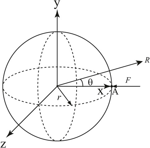
FIGURE 1. The excited sphere model, radius 1.2 m, thickness 0.012 m.
radius of the shell is 1.2 m,
thickness of the shell is 0.012 m,
elasticity modulus of the shell is 2.10 × 10¹¹ Pa.
Poisson’s ratio of the shell is 0.3,
structural density is 7.86 × 10³ kg/m3,
fluid density is 1.00 × 10³ kg/m3,
sound velocity in water is 1.482 × 10³ m/s.
The numerical and analytical solutions, expressed in terms of frequencies, for the sound pressure at point (2.4, 0, 0), are shown in Figure 2. The numerical and analytical solutions, expressed in terms of frequencies, for the sound power on the structural shell surface, are shown in Figure 3. The linear systems are solved using the GMRES implementation without preconditioning, and the wideband FMM algorithm is used to speed up the solving process. 6,144 elements make up the discretized thin-shell model. These figures both demonstrate the good agreement between the numerical and analytical solutions, demonstrating that the wideband FMM method preserves the excellent accuracy of traditional BEM.

FIGURE 2. Sound pressure at point (2.4, 0, 0).
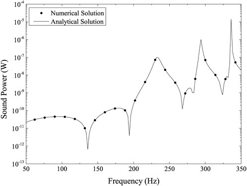
FIGURE 3. Sound power on the structural shell surface.
Figures 4, 5 depicts the structure surface’s sensitivity of sound pressure to the sphere’s radius and its shell thickness, respectively. Figures 6, 7 illustrates the structural surface’s sensitivity of sound power to the sphere’s radius and its shell thickness, respectively. These four figures show a remarkably similar pattern. These figures show that the numerical and analytical results accord rather well. The figures illustrate how the sound pressure or sound power sensitivity is very modest in the low-frequency range but substantially increases at resonance peaks.
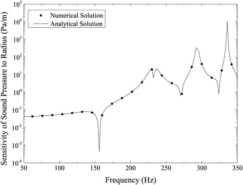
FIGURE 4. Sensitivity of sound pressure at point (2.4, 0, 0) to shell radius.
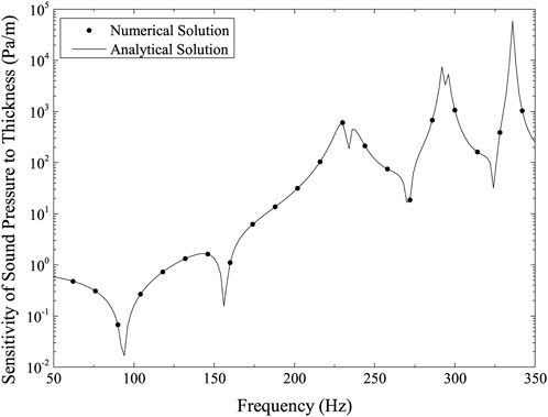
FIGURE 5. Sensitivity of sound pressure at point (2.4, 0, 0) to shell thickness.
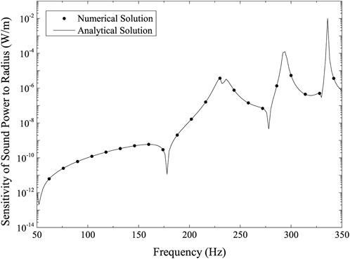
FIGURE 6. Structural surface’s sensitivity of sound power to shell radius.
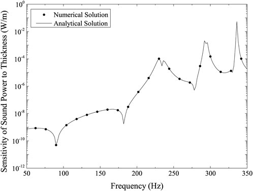
FIGURE 7. Structural surface’s sensitivity of sound power to shell thickness.
4.2 A BeTSSi-Sub submarine model under incident wave
The scattering sound field of the underwater submarine model under the influence of plane waves is the subject of this section. The incident wave amplitude is 1.0 Pa, and the plane wave propagates positively along the x-axis. The generic model BeTSSi-Sub presented at the World Digital Simulation Conference in 2002 is adopted by the model. The model has a 0.10 m thickness. The positive x-axis direction is from the bow to the stern, and the origin of the coordinate is located at the intersection of the circle that connects the bow and the hull. For the specific geometric characteristics of the BeTSSi-Sub model, please refer to Figure 3, 4 in [58]. Figure 8 displays the submarine model, with a total of 27,034 elements.
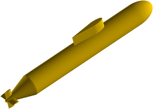
FIGURE 8. The BeTSSi-Sub submarine model.
The point for the computation is (40, 0, 0). Figure 9 shows the calculation result of sound pressure at point (40, 0, 0), and Figure 10 is the sensitivity of sound pressure at point (40, 0, 0) to shell thickness. Figures 9, 10 show that when the calculation frequency rises, both the sound pressure and its sensitivity to thickness gradually decline. Given that the sound pressure is significantly higher and more sensitive to changes in structural thickness in the lower frequency band, these two figures show that the lower frequency band is a crucial region for the BeTSSi-Sub model with the current material and geometrical specifications.
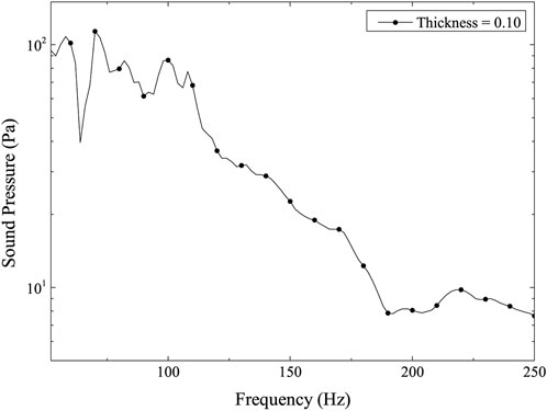
FIGURE 9. Sound pressure at point (40, 0, 0).
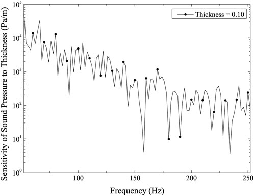
FIGURE 10. Sensitivity of sound pressure at point (40, 0, 0) to shell thickness.
5 Conclusion
The simulation of acoustic-structure interaction and sensitivity analysis is done using a coupling method based on FEM and BEM. Modelling the problem’s structural components is done using the FEM. The BEM is used to discretize the border of the acoustic domain, which is the boundary of the considered structure under consideration, in order to eliminate the necessity to mesh the acoustic domain. Boundary element analysis uses the FMM to speed up the matrix-vector products. Through the use of IGABEM, structural-acoustic interaction and its sensitivity analysis may be carried out straight from CAD models without the need for meshing, while also eradicating geometric flaws. Equations for the radiated sound power sensitivity are developed for fully linked structural-acoustic systems. The sensitivity of the sound power emitted on the structure surface is calculated using an adjoint operator technique. The sensitivity of the emitted sound power on any closed surface around the radiator is determined using the direct differentiation method. The formulas used to compute the derivative of the radiated sound power for various design factors are provided. Numerical illustrations are provided to show the precision and viability of the suggested approach. The suggested approach may be applied to large-scale practical situations to quantitatively forecast the impact of various design factors on the sound field. Future study will involve extending the created method to real-world engineering issues and using the structural-acoustic design sensitivity analysis to optimization challenges.
Data availability statement
The original contributions presented in the study are included in the article/Supplementary Material, further inquiries can be directed to the corresponding author.
Author contributions
Conceptualization, XC; Data curation, XC; Formal analysis, RC; Investigation, JZ; Methodology, XC and YX; Project administration, YX; Software, XC and WM; Supervision, YX; Validation, WM; Visualization, RC; Writing—original draft, XC and JZ. All authors have read and agreed to the published version of the manuscript.
Conflict of interest
The authors declare that the research was conducted in the absence of any commercial or financial relationships that could be construed as a potential conflict of interest.
Publisher’s note
All claims expressed in this article are solely those of the authors and do not necessarily represent those of their affiliated organizations, or those of the publisher, the editors and the reviewers. Any product that may be evaluated in this article, or claim that may be made by its manufacturer, is not guaranteed or endorsed by the publisher.
References
1. Junger MC, Feit D. Sound, structures, and their interaction, 225. Cambridge, MA: MIT press (1986).
2. Xu Y, Li H, Chen L, Zhao J, Zhang X. Monte Carlo based isogeometric stochastic finite element method for uncertainty quantization in vibration analysis of piezoelectric materials. Mathematics (2022) 10:1840. doi:10.3390/math10111840
3. Chen L, Lian H, Xu Y, Li S, Liu Z, Atroshchenko E, et al. Generalized isogeometric boundary element method for uncertainty analysis of time-harmonic wave propagation in infinite domains. Appl Math Model (2022) 114:360–78. doi:10.1016/j.apm.2022.09.030
4. Everstine GC, Henderson FM. Coupled finite element/boundary element approach for fluid-structure interaction. The J Acoust Soc America (1990) 87:1938–47. doi:10.1121/1.399320
5. Chen Z, Hofstetter G, Mang H. A Galerkin-type BE-FE formulation for elasto-acoustic coupling. Comput Methods Appl Mech Eng (1998) 152:147–55. Containing papers presented at the Symposium on Advances in Computational Mechanics. doi:10.1016/S0045-7825(97)00187-4
6. Marburg S. Developments in structural-acoustic optimization for passive noise control. Arch Comput Methods Eng (2002) 9:291–370. doi:10.1007/BF03041465
7. Schneider S. FE/FMBE coupling to model fluid-structure interaction. Int J Numer Methods Eng (2008) 76:2137–56. doi:10.1002/nme.2399
8. Brunner D, Junge M, Gaul L. A comparison of FE-BE coupling schemes for large-scale problems with fluid-structure interaction. Int J Numer Methods Eng (2009) 77:664–88. doi:10.1002/nme.2412
9. Merz S, Kinns R, Kessissoglou N. Structural and acoustic responses of a submarine hull due to propeller forces. J Sound Vibration (2009) 325:266–86. doi:10.1016/j.jsv.2009.03.011
10. Merz S, Kessissoglou N, Kinns R, Marburg S. Passive and active control of the radiated sound power from a submarine excited by propeller forces. J Ship Res (2013) 57:59–71. doi:10.5957/jsr.2013.57.1.59
11. Peters H, Kessissoglou N, Marburg S. Modal decomposition of exterior acoustic-structure interaction. J Acoust Soc America (2013) 133:2668–77. doi:10.1121/1.4796114
12. van Opstal T, van Brummelen E, van Zwieten G. A finite-element/boundary-element method for three-dimensional, large-displacement fluid-structure-interaction. Comput Methods Appl Mech Eng (2015) 284:637–63. Isogeometric Analysis Special Issue. doi:10.1016/j.cma.2014.09.037
13. Tadeu A, António J. Use of constant, linear and quadratic boundary elements in 3D wave diffraction analysis. Eng Anal Boundary Elem (2000) 24:131–44. doi:10.1016/S0955-7997(99)00064-8
14. Marburg S, Schneider S. Influence of element types on numeric error for acoustic boundary elements. J Comp Acous (2003) 11:363–86. doi:10.1142/S0218396X03001985
15. Trevelyan J. Use of discontinuous boundary elements for fracture mechanics analysis. Eng Anal Boundary Elem (1992) 10:353–8. doi:10.1016/0955-7997(92)90150-6
16. Florez W, Power H. Comparison between continuous and discontinuous boundary elements in the multidomain dual reciprocity method for the solution of the two-dimensional Navier-Stokes equations. Eng Anal Boundary Elem (2001) 25:57–69. doi:10.1016/S0955-7997(00)00051-5
17. Atkinson KE. The numerical solution of integral equations of the second kind. In: Cambridge monographs on applied and computational mathematics. Cambridge: University of Cambridge (1996).
18. Chen L, Chen H, Zheng C, Marburg S. Structural-acoustic sensitivity analysis of radiated sound power using a finite element/discontinuous fast multipole boundary element scheme. Int J Numer Methods Fluids (2016) 82:858–78. doi:10.1002/fld.4244
19. Greengard L, Rokhlin V. A fast algorithm for particle simulations. J Comput Phys (1987) 73:325–48. doi:10.1016/0021-9991(87)90140-9
20. Coifman R, Rokhlin V, Wandzura S. The fast multipole method for the wave equation: a pedestrian prescription. IEEE Antennas Propag Mag (1993) 35:7–12. doi:10.1109/74.250128
21. Schneider S. Application of fast methods for acoustic scattering and radiation problems. J Comp Acous (2003) 11:387–401. doi:10.1142/S0218396X03002012
22. Shen L, Liu YJ. An adaptive fast multipole boundary element method for three-dimensional acoustic wave problems based on the Burton-Miller formulation. Comput Mech (2007) 40:461–72. doi:10.1007/s00466-006-0121-2
23. Saad Y (2003). Iterative methods for sparse linear systems (SIAM). US: Society for Industrial and Applied Mathematics
24. Marburg S, Schneider S. Performance of iterative solvers for acoustic problems. Part I. Solvers and effect of diagonal preconditioning. Eng Anal Bound Elem (2003) 27:727–50. doi:10.1016/S0955-7997(03)00025-0
25. Gumerov NA, Duraiswami R. A broadband fast multipole accelerated boundary element method for the three dimensional Helmholtz equation. J Acoust Soc America (2009) 125:191–205. doi:10.1121/1.3021297
26. Wolf WR, Lele SK. Wideband fast multipole boundary element method: Application to acoustic scattering from aerodynamic bodies. Int J Numer Methods Fluids (2011) 67:2108–29. doi:10.1002/fld.2486
27. Dühring MB, Jensen JS, Sigmund O. Acoustic design by topology optimization. J Sound Vibration (2008) 317:557–75. doi:10.1016/j.jsv.2008.03.042
28. Hughes T, Cottrell J, Bazilevs Y. Isogeometric analysis: CAD, finite elements, NURBS, exact geometry and mesh refinement. Comput Methods Appl Mech Eng (2005) 194:4135–95. doi:10.1016/j.cma.2004.10.008
29. Simpson R, Bordas S, Trevelyan J, Rabczuk T. A two-dimensional isogeometric boundary element method for elastostatic analysis. Comput Methods Appl Mech Eng (2012) 209-212:87–100. doi:10.1016/j.cma.2011.08.008
30. Simpson R, Bordas S, Lian H, Trevelyan J. An isogeometric boundary element method for elastostatic analysis: 2D implementation aspects. Comput Struct (2013) 118:2–12. Issue: UK Association for Computational Mechanics in Engineering. doi:10.1016/j.compstruc.2012.12.021
31. Scott M, Simpson R, Evans J, Lipton S, Bordas S, Hughes T, et al. Isogeometric boundary element analysis using unstructured T-splines. Comput Methods Appl Mech Eng (2013) 254:197–221. doi:10.1016/j.cma.2012.11.001
32. Chen L, Lian H, Natarajan S, Zhao W, Chen X, Bordas S. Multi-frequency acoustic topology optimization of sound-absorption materials with isogeometric boundary element methods accelerated by frequency-decoupling and model order reduction techniques. Comput Methods Appl Mech Eng (2022) 395:114997. doi:10.1016/j.cma.2022.114997
33. Chen L, Wang Z, Peng X, Yang J, Wu P, Lian H. Modeling pressurized fracture propagation with the isogeometric bem. Geomech Geophys Geo Energ Ge Resour (2021) 7:51. doi:10.1007/s40948-021-00248-3
34. Xu G, Mourrain B, Duvigneau R, Galligo A. Parameterization of computational domain in isogeometric analysis: Methods and comparison. Comput Methods Appl Mech Eng (2011) 200:2021–31. doi:10.1016/j.cma.2011.03.005
35. Xu G, Li M, Mourrain B, Rabczuk T, Xu J, Bordas SP. Constructing IGA-suitable planar parameterization from complex CAD boundary by domain partition and global/local optimization. Comput Methods Appl Mech Eng (2018) 328:175–200. doi:10.1016/j.cma.2017.08.052
36. Kostas K, Ginnis A, Politis C, Kaklis P. Ship-hull shape optimization with a T-spline based BEM-isogeometric solver. Comput Methods Appl Mech Engisogeometric Anal Spec Issue (2015) 284:611–22. doi:10.1016/j.cma.2014.10.030
37. Lian H, Kerfriden P, Bordas S. Shape optimization directly from CAD: An isogeometric boundary element approach using T-splines. Comput Methods Appl Mech Eng (2017) 317:1–41. doi:10.1016/j.cma.2016.11.012
38. Li S, Trevelyan J, Wu Z, Lian H, Wang D, Zhang W. An adaptive SVD-Krylov reduced order model for surrogate based structural shape optimization through isogeometric boundary element method. Comput Methods Appl Mech Eng (2019) 349:312–38. doi:10.1016/j.cma.2019.02.023
39. Simpson R, Scott M, Taus M, Thomas D, Lian H. Acoustic isogeometric boundary element analysis. Comput Methods Appl Mech Eng (2014) 269:265–90. doi:10.1016/j.cma.2013.10.026
40. Chen L, Liu C, Zhao W, Liu L. An isogeometric approach of two dimensional acoustic design sensitivity analysis and topology optimization analysis for absorbing material distribution. Comput Methods Appl Mech Eng (2018) 336:507–32. doi:10.1016/j.cma.2018.03.025
41. Chen L, Lian H, Liu Z, Chen H, Atroshchenko E, Bordas S. Structural shape optimization of three dimensional acoustic problems with isogeometric boundary element methods. Comput Methods Appl Mech Eng (2019) 355:926–51. doi:10.1016/j.cma.2019.06.012
42. Chen L, Lu C, Lian H, Liu Z, Zhao W, Li S, et al. Acoustic topology optimization of sound absorbing materials directly from subdivision surfaces with isogeometric boundary element methods. Comput Methods Appl Mech Eng (2020) 362:112806. doi:10.1016/j.cma.2019.112806
43. Peng X, Atroshchenko E, Kerfriden P, Bordas S. Isogeometric boundary element methods for three dimensional static fracture and fatigue crack growth. Comput Methods Appl Mech Eng (2017) 316:151–85. Special Issue on Isogeometric Analysis: Progress and Challenges. doi:10.1016/j.cma.2016.05.038
44. Peng X, Atroshchenko E, Kerfriden P, Bordas S. Linear elastic fracture simulation directly from CAD: 2D NURBS-based implementation and role of tip enrichment. Int J Fract (2017) 204:55–78. doi:10.1007/s10704-016-0153-3
45. Zhang J, Zhang W, Zhu J, Xia L. Integrated layout design of multi-component systems using XFEM and analytical sensitivity analysis. Comput Methods Appl Mech Eng (2012) 245-246:75–89. doi:10.1016/j.cma.2012.06.022
46. Lamancusa J. Numerical optimization techniques for structural-acoustic design of rectangular panels. Comput Structures (1993) 48:661–75. doi:10.1016/0045-7949(93)90260-K
47. Hambric SA. Sensitivity calculations for broad-band Acoustic radiated noise design optimization problems. J Vib Acoust (1996) 118:529–32. doi:10.1115/1.2888219
48. Marburg S, Hardtke H-J. Shape optimization of a vehicle hat-shelf: improving acoustic properties for different load cases by maximizing first eigenfrequency. Comput Structures (2001) 79:1943–57. doi:10.1016/S0045-7949(01)00107-9
49. Haftka RT, Adelman HM. Recent developments in structural sensitivity analysis. Struct Optimization (1989) 1:137–51. doi:10.1007/BF01637334
50. Marburg S. Efficient optimization of a noise transfer function by modification of a shell structure geometry - Part I: Theory. Struct Multidiscipl Optim (2002) 24:51–9. doi:10.1007/s00158-002-0213-3
51. Fritze D, Marburg S, Hardtke H-J. FEM-BEM-coupling and structural-acoustic sensitivity analysis for shell geometries. Comput Struct (2005) 83:143–54. doi:10.1016/j.compstruc.2004.05.019
52. Choi K, Shim I, Wang S. Design sensitivity analysis of structure-induced noise and vibration. J Vib Acoust (1997) 119:173–9. doi:10.1115/1.2889699
53. Wang S. Design sensitivity analysis of noise, vibration, and harshness of vehicle body structure. Mech Structures Machines (1999) 27:317–35. doi:10.1080/08905459908915701
54. Cirak F, Ortiz M, Schröder P. Subdivision surfaces: a new paradigm for thin-shell finite-element analysis. Int J Numer Methods Eng (2000) 47:2039–72. doi:10.1002/(SICI)1097-0207(20000430)47:12<2039::AID-NME872>3.0.CO;2-1
56. Chen L, Cheng R, Li S, Lian H, Zheng C, Bordas S. A sample-efficient deep learning method for multivariate uncertainty qualification of acoustic–vibration interaction problems. Comput Methods Appl Mech Eng (2022) 393:114784. doi:10.1016/j.cma.2022.114784
57. Chen L, Lian H, Liu Z, Gong Y, Zheng C, Bordas S. Bi-material topology optimization for fully coupled structural-acoustic systems with isogeometric fem–bem. Eng Anal Boundary Elem (2022) 135:182–95. doi:10.1016/j.enganabound.2021.11.005
Keywords: iga, FEM/BEM, structural-acoustic coupling, sound power, sensitivity analysis
Citation: Chen X, Xu Y, Zhao J, Cheng R and Ma W (2022) Sensitivity analysis of structural-acoustic fully-coupled system using isogeometric boundary element method. Front. Phys. 10:1082824. doi: 10.3389/fphy.2022.1082824
Received: 28 October 2022; Accepted: 15 November 2022;
Published: 30 November 2022.
Edited by:
Pei Li, Xi’an Jiaotong University, ChinaReviewed by:
Yunfei Gao, Hohai University, ChinaChuang Lu, University of Science and Technology of China, China
Copyright © 2022 Chen, Xu, Zhao, Cheng and Ma. This is an open-access article distributed under the terms of the Creative Commons Attribution License (CC BY). The use, distribution or reproduction in other forums is permitted, provided the original author(s) and the copyright owner(s) are credited and that the original publication in this journal is cited, in accordance with accepted academic practice. No use, distribution or reproduction is permitted which does not comply with these terms.
*Correspondence: Yanming Xu, eHV5YW5taW5nQHVzdGMuZWR1