- 1School of Information and Control Engineering, Qingdao University of Technology, Qingdao, China
- 2School of Science, Qingdao University of Technology, Qingdao, China
The ideal Hopfield network would be able to remember information and recover the missing information based on what has been remembered. It is expected to have applications in areas such as associative memory, pattern recognition, optimisation computation, parallel implementation of VLSI and optical devices, but the lack of memory capacity and the tendency to generate pseudo-attractors make the network capable of handling only a very small amount of data. In order to make the network more widely used, we propose a scheme to optimise and improve its memory and resilience by introducing quantum perceptrons instead of Hebbian rules to complete its weight matrix design. Compared with the classical Hopfield network, our scheme increases the threshold of each node in the network while training the weights, and the memory space of the Hopfield network changes from being composed of the weight matrix only to being composed of the weight matrix and the threshold matrix together, resulting in a dimensional increase in the memory capacity of the network, which greatly solves the problem of the Hopfield network’s memory The problem of insufficient memory capacity and the tendency to generate pseudo-attractors was solved to a great extent. To verify the feasibility of the proposed scheme, we compare it with the classical Hopfield network in four different dimensions, namely, non-orthogonal simple matrix recovery, incomplete data recovery, memory capacity and model convergence speed. These experiments demonstrate that the improved Hopfield network with quantum perceptron has significant advantages over the classical Hopfield network in terms of memory capacity and recovery ability, which provides a possibility for practical application of the network.
1 Introduction
Machine learning [1] is an important branch of artificial intelligence and a way to achieve artificial intelligence, i.e. machine learning is used as a means to solve problems in artificial intelligence. It is a multi-disciplinary discipline involving probability theory, statistics convex optimisation, complexity theory and many other disciplines. Machine learning algorithms are a class of algorithms that analyse existing data to obtain a certain pattern and use this pattern to make predictions about unknown data. It has been used with great success in very many fields, including medicine [2], biology [3], chemistry [4], physics [5–8] and mathematics [9]. Machine learning has proven to be one of the most successful ways to explore the field of artificial intelligence.
Perceptron [10] is a two-classification linear classification model, which aims to find the hyperplane that divides the training data linearly. Its biggest feature is that it is easy to implement. Suppose the training data set is
Where
The linear equation

FIGURE 1. Models of classical perceptual machines (left) and applications to classification (right).
Quantum information is a new discipline developed based on quantum physics and information technology, which mainly includes two fields: quantum communication and quantum computing. Quantum communication focuses on quantum cryptography [11,12], quantum teleportation [13–16], and quantum direct communication [17], while quantum computing focuses on algorithms that fit quantum properties [18–23]. This is an extremely active field, as it has the potential to disrupt classical informatics, communication technologies, and computing methods.
Quantum perceptron belongs to quantum machine learning algorithms [24,25], which is the quantum counterpart of the classical perceptron model. Kapoor proved that quantum computation can provide significant improvements in the computational and statistical complexity of the perceptron model [26]; Schuld proposed a scalable quantum perceptron based on quantum Fourier transform [27], which can be used as a component of other more advanced networks [28]; Tacchino proposed a quantum perceptron model that can run on near-term quantum processing hardwar [29]. Currently, quantum perceptron models are in the exploratory stage and there is no absolute authority on them. In our work, the quantum perceptron model based on the quantum phase estimation algorithm [27] proposed by Schuld is used. The inverse quantum Fourier transform and the gradient descent algorithm on a classical computer are used to train the weight matrix of the perceptron.
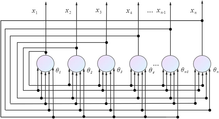
Hopfield network (HNN) are single-layer full feedback network [30], which are characterised by the fact that the output xi of any neuron is fed back to all neurons xj as output by connecting the weights wij. The network usually uses Hebbian rule [31] for the design of the weight matrix. Hebbian rule is simpler but useful for the design of the weight matrix in HNN. However, sometimes the Hebbian rule cannot find an exact weight matrix, even though such a matrix exists [32]. This is because the rule does not incorporate the thresholds of the HNN into the training, which can result in attractors producing ranges of attraction domains that overlap each other or even appear to overwrite. And if the vectors to be stored are closer to each other, their probability of error is higher.
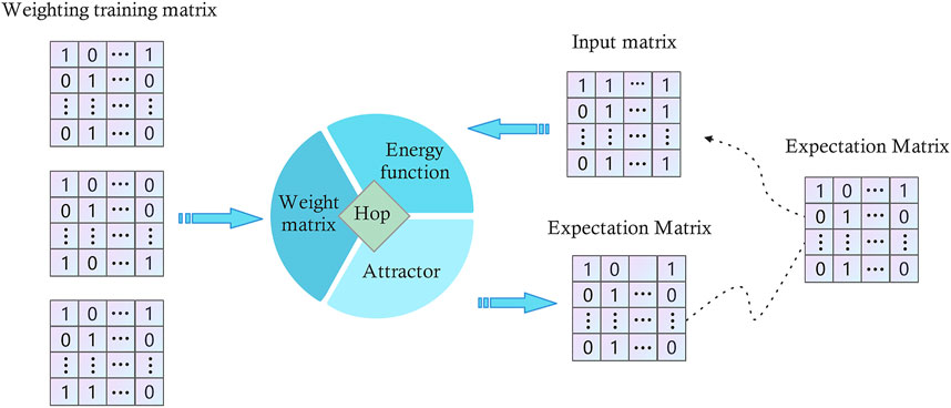
Considering that the weight matrix designed by the Hebbian rule is not enough to support the HNN to accomplish various practical tasks, we propose an improvement scheme, which will use the quantum perceptron instead of the Hebbian rule for the design of the HNN weights, Firstly, the weights and thresholds of the Hopfield network are mapped into the weight matrix of the quantum perceptron, and each node of the HNN is used as the input vector, and the weight matrix of the quantum perceptron is passed through the quantum The final weight matrix of the quantum perceptron is the weight matrix and threshold matrix of the HNN. The improved HNN has more memory storage space than the Hebbian rule because it has an additional threshold matrix to assist in storage, and can store the memorised information better. Moreover, due to the more accurate weight information, it is also easier to reach the steady state when iterating the HNN, thus the resilience and model convergence speed are significantly improved. Currently, the most widespread use of HNNs is for information recovery and information matching. Our improved HNN has been simulated and analysed to provide a huge improvement over the classical HNN in both information recovery and information matching, which makes the improved HNN more usable than the classical HNN, which is expected to provide more applications for HNNs in more fields, such as playing a greater role in virus information identification, human brain simulation, and error correction of quantum noise [33].
In Section 2, we describe in detail the HNN model, the Hebbian rule, the quantum Fourier transform and the quantum phase estimation algorithm used in this paper; Section 3 describes in detail the theory of our approach, including the correspondence between the HNN and the perceptron model, the quantum perceptron model and how to use the quantum perceptron model for training the HNN weights and thresholds; Section 4 presents our simulation Section 4 presents our experimental analysis, in which we design experiments to verify the feasibility of our proposed scheme and its improvement and advantages over the classical scheme; Section 5 concludes the paper and provides predictions and analysis of the future of our proposed scheme.
2 Preliminaries
2.1 Hopfield network
HNN are multi-input, thresholded, binary nonlinear dynamic systems. The excitation function of the neuron is usually a step function, and the value of the neuron is −1, 1, or 0,1. When the value is 0 or −1, the current neuron is in the inhibited state, and when the value is 1, the current neuron is in the activated state. The HNN is a single layer neural network in which all neuron nodes are connected to other neuron nodes. There is no self-feedback between the nodes, forming a complete graph model. A neuron node in the inhibited state will enter the activated state when the stimulus exceeds a set threshold, i.e. it will jump from 0 or −1 to 1.
Each node in a HNN has the same function, and the output of a single node corresponds to the final state of that node, denoted by xi, with the states of all nodes forming the state of the network
where
2.2 Hebbian rule
The Hebbian rule describes the basic principle of synaptic plasticity, that is, continuous and repeated stimulation from presynaptic neurons to postsynaptic neurons can increase the efficiency of synaptic transmission.
The Hebbian rule is the oldest and simplest neuron learning rule. Here is the description equantion of the Hebbian rule:
Where wij is the connection weight from neuron j to neuron i, p is the number of training modes, and
In the HNN, Hebbian rules can be used to design weight matrices:
Here wii = 0, which means that there is no self-feedback between nodes. The equantion is rewritten as follows:
Where I is the unit matrix and X is the system state of HNN.
2.3 HNN attractor and pseudo attractor
Considering that the Hopfield network has M samples of Xm, then:
Because of n
According to Eq. 9: when a given sample, Xm is the ideal attractor and produces a certain attractor domain around it, which will be “captured” by the attractor in the attractor domain. However, the condition that the given samples are orthogonal to each other is too harsh, which eventually leads to the attraction domain of some points outside the samples, which are regarded as pseudo attractors of the HNN.
2.4 Quantum Fourier transform
The quantum Fourier transform is an efficient quantum algorithm for the Fourier transform of quantum amplitudes. The quantum Fourier transform is not the classical counterpart of the Fourier transform and does not speed up the Fourier transform process on classical data, but it can perform an important task-phase estimation, i.e. estimating the eigenvalues of the You operator under certain conditions. The matrix representation of the quantum Fourier transform is as follows:
Where,
In the classical Fourier transform, the transformation takes the following form:
The mathematical form of the quantum Fourier transform is similar to the mathematical representation of the discrete Fourier transform [34]. It is an operator defined on a set of standard orthogonal bases |0⟩, |1⟩⋯|N − 1⟩ with the following action:
An arbitrary quantum state action can be expressed as:
where the amplitude
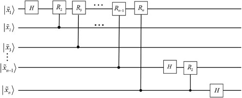
The transform itself does not have much obvious value, but it is an important component subalgorithm of the quantum phase estimation algorithm. The quantum Fourier transform corresponds to the quantum line diagram (omitting the SWAP gate), where
2.5 Qunamtum phase estimation algorithm
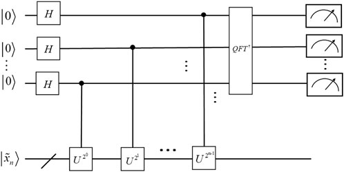
The quantum phase estimation algorithm is the key to many quantum algorithms [6,35], and its role is to estimate the phase in the eigenvalues of the eigenvectors corresponding to the You matrix. The quantum circuit for quantum phase estimation is shown in Figure 4. The algorithm uses two registers, the first of which contains τ quantum bits with initial state |0⟩. The value of τ depends on the number of bits desired to be accurately estimated and the desired success rate. The second register has an initial state of
where state
3 Methods
3.1 Correspondence between perceptron models and HNN
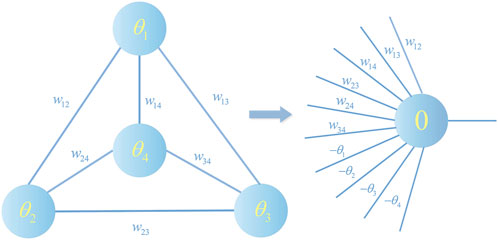
Firstly, we will discuss HNN with the range restricted to cells with non-zero thresholds and a step function as the threshold function, which is by far the most common form of HNN. Secondly two consensus needs to be established: 1) the units in this network are perceptrons. 2) The perceptron can determine the weights and thresholds of the network for the problem to be learned. Focus on consensus i): Based on the definitions of HNN and perceptual machines above, it is clear that the unit in a HNN is a perceptual machine.
Focus on consensus ii): Consider a HNN with n cells, where W is the weight matrix of n × n, such that θi denotes the threshold of the cell i and the state of the network is X. If one wants this network to reach a steady state, it means that the following n inequalities must be satisfied:
Since it has no self-feedback, only the n (n − 1)/2 non-zero entries of the weight matrix W and the n thresholds of the cells appear in these inequalities. Let u denote the vector of n + n (n + 1)/2 dimension whose components are the non-diagonal elements of the weight matrix wij (i < j) and the n threshold minus signs. The vector u is given by the following equation:
The vector x is transformed into n auxiliary vectors v1, v2, v3, … , vn of dimension n + n (n + 1)/2 given by the expression:
3.2 Quantum perceptron model
First, t-qubit state|0⟩ are passed through the Hadmard gate, to obtain the superposition state
Where
Finally the estimated phase can be obtained by inverse Fourier transform
3.3 Obtaining parameter information using quantum perception
The connection between the HNN and the perceptron model was described above. It is now clarified how the design of the HNN weight matrix can be carried out using the quantum perceptron. Firstly, σ = (v, u) is input to the quantum perceptron model as an initial parameter and the model update rule for the quantum perceptron is as follows:
From the above equation, it can be deduced that |σ⟩ is an eigenvector of the matrix U and e2πiΔϕh(u,v) is the corresponding eigenvalue. By picking the appropriate value of t in the quantum perceptron, the inverse Fourier transform by:
It is possible to obtain a value of, which is very close to the true phase, and also becomes closer to the true phase as the value of t becomes larger. Combining Eq. 19 gives:
Therefore the value of σ = (v, u) can be obtained by
where
3.4 Computational complexity analysis
We analyze the computational complexity of the HNN in two steps. 1) Analysis of the lift rate of the data to be trained after conversion of the HNN to the perceptron model. 2) The computational complexity required to complete the weight parameters by means of the quantum phase estimation algorithm. First we analyse i), any HNN with n nodes satisfying the requirements of Section 3.1 can be converted into a perceptron model with n (n − 1)/2 weight parameters. For ii), we analyze here two different algorithms for finding the weight parameters, namely the gradient descent-based algorithm and the Grover fast weight finding algorithm. The time complexity of the gradient descent-based algorithm is mainly controlled by the number of steps ɛ accuracy, i.e. O ∝ ɛ2; the time complexity of finding the parameters using the Grover algorithm can reach O(n) under certain conditions. It is clear from this analysis that the final computational complexity is
4 Emulation analysis
The two most important applications of HNN are data matching and data recovery, which correspond to the accuracy of the HNN’s weight matrix and memory capacity respectively. The convergence speed of the HNN model is extremely important in both data matching and data recovery. To this end, we designed three experiments, namely a non-orthogonal simple matrix recovery test, a Random binary-based incomplete matrix recovery test, and a memory capacity test based on the recognizability of QR codes, to compare the effectiveness of our proposed improved HNN with that of the classical HNN, and finally we added a model convergence speed comparison experiment to compare the performance differences between the models.
Our simulation analysis is based on the pennylane open source framework. The framework has embedded transition algorithms between quantum and classical algorithms as well as parameter optimisation algorithms, eliminating the need for us to package the parameters and design the optimisation algorithms separately. With this framework, the measured and calculated weight parameters are directly updated iteratively by means of a gradient descent algorithm, and the relevant information is fed back into the quantum algorithm to update the perceptron weights. Using this as a basis, we have designed the following simulation experiments.
4.1 Result
In the non-orthogonal simple matrix memory test, we demonstrated that our proposed solution can effectively cope with the memory confusion caused by non-orthogonal simple matrices; in the fragmented data recovery test, we demonstrated that our proposed QP-HNN has an average recovery rate improvement of 30.6% and a maximum of 49.1% in the effective interval compared with Hebbian rule-Hopfield network (HR-HNN), making it more practical. In the memory stress test based on QR code recognisability, our proposed QP-HNN is 2.25 times more effective than HR-HNN.
4.2 Non-orthogonal simple matrix memory test
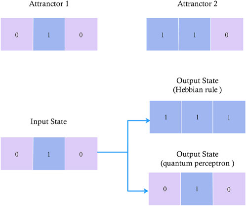
The non-orthogonal simple matrix memory test is set up for the Hebbian rule in the classical HNN, as one of the prerequisites for the design of the weight matrix using the Hebbian rule is that the input vectors must be orthogonal to each other, and if they do not satisfy orthogonality, the designed weight matrix may be incorrect. We demonstrate the impact of this deficiency using two non-orthogonal 3D row vectors Xv = [0, 1, 0] and Xϑ = [1, 1, 1] as the input matrices for HR-HNN and QP-HNN, as shown in Figure 6 Where the trained weight matrix WHR = [[0, 1, 1] [1, 0, 1] [1, 1, 0]] for HR-HNN, the weight matrix WQP = [[0, 0.5, 0.3] [0.5, 0, 0] [0, 0, 0.2]] for QP − Hop and the threshold matrix θQP = [0.6, −0.1, 0.2].
4.3 Random binary-based incomplete matrix recovery test
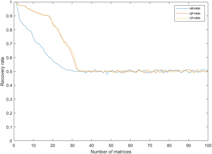
In this subsection, we test and compare the recoverability of three different HNN: ClassicalPerceptron-Hopfield (CP-HNN), QP-HNN, and HR-HNN. Firstly, a random number generator was used to generate 100 60 × 60 binary matrices
From Figure 8, it can be seen that the resilience of the HR-HNN network decreases rapidly as ι becomes larger ι means that the orthogonality between the matrices in Mι decreases, and consequently, memory confusion ensues. The resilience of the network basically fails at ι = 20 and is completely lost at ι = 30; the ClassicalPerceptron-Hopfield (CP-HNN) network is highly similar to the QP-HNN network in terms of resilience and has excellent robustness in the first and middle stages of ι growth because the network also trains the threshold This is equivalent to increasing the error tolerance space and mitigating errors due to the non-orthogonality of the vectors in the matrix. As can be seen from the diagram, the network is still very resilient at ι = 20. However, as ι increases, the fault tolerance space becomes saturated and the resilience decreases rapidly until it fails.
4.4 Memory capacity test based on the recognizability of QR codes
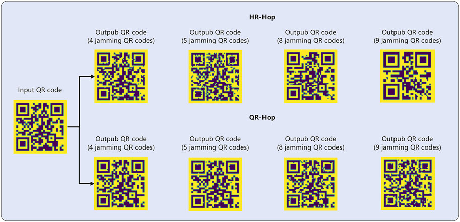
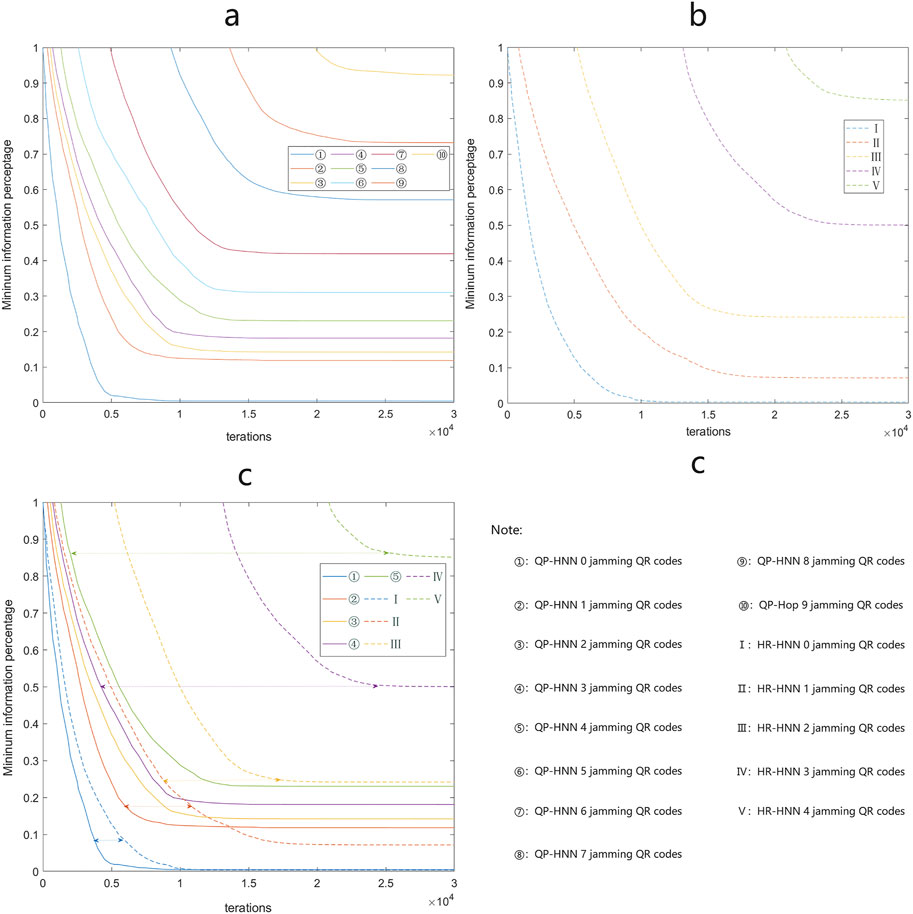
In order to visualise the memory capacity of the models, the differences between the models are presented using QR codes, which have different levels of fault tolerance and represent the number of error pixels that can be tolerated in the QR code. For our tests we have used the L level of fault tolerance, which allows for a maximum of 7% of incorrect pixels.
The QR code q1 is generated and stored in the “Successful Identification”, generating a QR code set
4.5 HNN recovery rate test
The usability of HNN is also affected by the number of iterations required for the model to converge, which in turn is affected by the completeness of the weights, threshold information and input data. Therefore, building on the previous subsection, we further investigate the number of iterations required for q′ to recover to the state
Table 1 counts the recovery capacity limit of the HNN when the preset upper limit of 30,000 iterations is reached, where HR-HNN reaches the memory limit at m = 4, i.e. at m = 5, q′ cannot recover to
5 Conclusion
We improve the original HNN weight design method by using a quantum perceptron instead of the Hebbian rule. The improved QP-HNN can better handle non-orthogonal matrices, and its information memory and recovery capabilities as well as model convergence speed are significantly improved compared to HR-HNN. It also opens up the possibility of further expanding the scope of applications in areas such as virus information recognition, human brain simulation, and error correction of quantum noise.
Our improved scheme is based on the quantum perceptron model proposed that we can input all the data to be processed into the model simultaneously by transforming and preparing them into quantum entangled states. The current model used is still the quantum-classical computing model, where the optimal weighting parameters are found by a classical computer, but Kapoor et al. have shown that the weighting parameters can be found much faster using the Grover algorithm, considerably increase the efficiency of finding the weight parameters to compensate for the extra time consumed in its determination of the weights compared to the Hebbian rule. Currently, corresponding quantum models of HNNs already exist, and the combination of quantum perceptrons and quantum HNNs is also destined to be more desirable in pure quantum computers than in classical HNNs.
Data availability statement
The raw data supporting the conclusions of this article will be made available by the authors, without undue reservation.
Author contributions
ZS: Conceptualization, Methodology, Software,Writing-Original draft preparation. YQ: Data curation, Writing-Original draft preparation. ML: Visualization, Investigation. JL:Supervision, Writing—Review and Editing. HM: Supervision, Writing—Review and Editing, Project administration, Funding acquisition.
Funding
Project supported by the National Natural Science Foundation of China (Grant Nos. 61772295), Natural Science Foundation of Shandong Province, China (Grant Nos. ZR2021MF049, ZR2019YQ01), Project of Shandong Provincial Natural Science Foundation Joint Fund Application (ZR202108020011).
Conflict of interest
The authors declare that the research was conducted in the absence of any commercial or financial relationships that could be construed as a potential conflict of interest.
Publisher’s note
All claims expressed in this article are solely those of the authors and do not necessarily represent those of their affiliated organizations, or those of the publisher, the editors and the reviewers. Any product that may be evaluated in this article, or claim that may be made by its manufacturer, is not guaranteed or endorsed by the publisher.
References
1. Carleo G, Cirac I, Cranmer K, Daudet L, Schuld M, Tishby N, et al. Machine learning and the physical sciences. Rev Mod Phys (2019) 91:045002. doi:10.1103/RevModPhys.91.045002
2. Liakos KG, Busato P, Moshou D, Pearson S, Bochtis D. Machine learning in agriculture: A review. Sensors (2018) 18:2674. doi:10.3390/s18082674
3. Pinter G, Felde I, Mosavi A, Ghamisi P, Gloaguen R. Covid-19 pandemic prediction for Hungary; a hybrid machine learning approach. Mathematics (2020) 8:890. doi:10.3390/math8060890
4. Dral PO. Quantum chemistry in the age of machine learning. J Phys Chem Lett (2020) 11:2336–47. doi:10.1021/acs.jpclett.9b03664
5. Radovic A, Williams M, Rousseau D, Kagan M, Bonacorsi D, Himmel A, et al. Machine learning at the energy and intensity frontiers of particle physics. Nature (2018) 560:41–8. doi:10.1038/s41586-018-0361-2
6. Haug T, Dumke R, Kwek L-C, Miniatura C, Amico L. Machine-learning engineering of quantum currents. Phys Rev Res (2021) 3:013034. doi:10.1103/PhysRevResearch.3.013034
7. Zhang L, Chen Z, Fei SM. Einstein-podolsky-rosen steering based on semisupervised machine learning. Phys Rev A (Coll Park) (2021) 104:052427. doi:10.1103/PhysRevA.104.052427
8. Jasinski A, Montaner J, Forrey RC, Yang BH, Stancil PC, Balakrishnan N, et al. Machine learning corrected quantum dynamics calculations. Phys Rev Res (2020) 2:032051. doi:10.1103/PhysRevResearch.2.032051
9. Jumper J, Evans R, Pritzel A, Green T, Figurnov M, Ronneberger O, et al. Highly accurate protein structure prediction with alphafold. Nature (2021) 596:583–9. doi:10.1038/s41586-021-03819-2
10. Rosenblatt F. The perceptron: A probabilistic model for information storage and organization in the brain. Psychol Rev (1958) 65:386–408. doi:10.1037/h0042519
11. Zhou N, Hu Y, Gong L, Li G. Quantum image encryption scheme with iterative generalized arnold transforms and quantum image cycle shift operations. Quan Inf Process (2017) 16:164–23. doi:10.1007/s11128-017-1612-0
12. Yi Nuo W, Zhao Yang S, Yu Lin M, Nan H, Hong Yang M. Color image encryption algorithm based on dna code and alternating quantum random walk. Acta Phys Sin (2021) 70:230302–23. doi:10.7498/aps.70.20211255
13. Ye TY, Geng MJ, Xu TJ, Chen Y. Efficient semiquantum key distribution based on single photons in both polarization and spatial-mode degrees of freedom. Quan Inf Process (2022) 21:123–1. doi:10.1007/s11128-022-03457-1
14. Ma HY, Guo ZW, Fan XK, Wang SM. The routing communication protocol for small quantum network based on quantum error correction code. Acta Electonica Sinica (2015) 43:171. doi:10.3969/j.issn.0372-2112.2015.01.027
15. Zhou NR, Zhu KN, Zou XF. Multi-party semi-quantum key distribution protocol with four-particle cluster states. Annalen der Physik (2019) 531:1800520. doi:10.1002/andp.201800520
16. Ye TY, Li HK, Hu JL. Semi-quantum key distribution with single photons in both polarization and spatial-mode degrees of freedom. Int J Theor Phys (Dordr) (2020) 59:2807–15. doi:10.1007/s10773-020-04540-y
17. Sheng YB, Zhou L, Long GL. One-step quantum secure direct communication. Sci Bull (2022) 67:367–74. doi:10.1016/j.scib.2021.11.002
18. Noiri A, Takeda K, Nakajima T, Kobayashi T, Sammak A, Scappucci G, et al. Fast universal quantum gate above the fault-tolerance threshold in silicon. Nature (2022) 601:338–42. doi:10.1038/s41586-021-04182-y
19. Lloyd S, Mohseni M, Rebentrost P. Quantum principal component analysis. Nat Phys (2014) 10:631–3. doi:10.1038/nphys3029
20. Li Z, Liu X, Xu N, Du J. Experimental realization of a quantum support vector machine. Phys Rev Lett (2015) 114:140504. doi:10.1103/PhysRevLett.114.140504
21. Low GH, Yoder TJ, Chuang IL. Quantum inference on bayesian networks. Phys Rev A (Coll Park) (2014) 89:062315. doi:10.1103/PhysRevA.89.062315
22. Dong D, Chen C, Li H, Tarn T-J. Quantum reinforcement learning. IEEE Trans Syst Man Cybern B (2008) 38:1207–20. doi:10.1109/TSMCB.2008.925743
23. Zhou N, Zhang TF, Xie XW, Wu JY. Hybrid quantum–classical generative adversarial networks for image generation via learning discrete distribution. Signal Processing: Image Commun (2022) 2022:116891. doi:10.1016/j.image.2022.116891
24. Biamonte J, Wittek P, Pancotti N, Rebentrost P, Wiebe N, Lloyd S. Quantum machine learning. Nature (2017) 549:195–202. doi:10.1038/nature23474
25. Harrow AW, Hassidim A, Lloyd S. Quantum algorithm for linear systems of equations. Phys Rev Lett (2009) 103:150502. doi:10.1103/PhysRevLett.103.150502
27. Weinstein YS, Pravia M, Fortunato E, Lloyd S, Cory DG. Implementation of the quantum Fourier transform. Phys Rev Lett (2001) 86:1889–91. doi:10.1103/PhysRevLett.86.1889
28. Schuld M, Sinayskiy I, Petruccione F. Simulating a perceptron on a quantum computer. Phys Lett A (2015) 379:660–3. doi:10.1016/j.physleta.2014.11.061
29. Tacchino F, Macchiavello C, Gerace D, Bajoni D. An artificial neuron implemented on an actual quantum processor. Npj Quan Inf (2019) 5:26–8. doi:10.1038/s41534-019-0140-4
30. Hopfield JJ. Neural networks and physical systems with emergent collective computational abilities. Proc Natl Acad Sci U S A (1982) 79:2554–8. doi:10.1073/pnas.79.8.2554
31. Hebb DO. The organization of behavior: A neuropsychological theory. London: Psychology Press (2005). doi:10.4324/9781410612403
32. Wuensche A. Discrete dynamical networks and their attractor basins. Complex Syst (1998) 98:3–21.
33. Wang H, Song Z, Wang Y, Tian Y, Ma H. Target-generating quantum error correction coding scheme based on generative confrontation network. Quan Inf Process (2022) 21:280–17. doi:10.1007/s11128-022-03616-4
34. Harris FJ. On the use of windows for harmonic analysis with the discrete Fourier transform. Proc IEEE (1978) 66:51–83. doi:10.1109/PROC.1978.10837
Keywords: hopfield network, weight matrix, quantum perceptron, storage capacity, recovery capability
Citation: Song Z, Qu Y, Li M, Liang J and Ma H (2022) Partial quantisation scheme for optimising the performance of hopfield network. Front. Phys. 10:1079624. doi: 10.3389/fphy.2022.1079624
Received: 25 October 2022; Accepted: 07 November 2022;
Published: 24 November 2022.
Edited by:
Tianyu Ye, Zhejiang Gongshang University, ChinaCopyright © 2022 Song, Qu, Li, Liang and Ma. This is an open-access article distributed under the terms of the Creative Commons Attribution License (CC BY). The use, distribution or reproduction in other forums is permitted, provided the original author(s) and the copyright owner(s) are credited and that the original publication in this journal is cited, in accordance with accepted academic practice. No use, distribution or reproduction is permitted which does not comply with these terms.
*Correspondence: Junqing Liang, bGlhbmdqdW5xaW5nQHF1dC5lZHUuY24=; Hongyang Ma, aG9uZ3lhbmdfbWFAYWxpeXVuLmNvbQ==
 Zhaoyang Song1
 Hongyang Ma