
94% of researchers rate our articles as excellent or good
Learn more about the work of our research integrity team to safeguard the quality of each article we publish.
Find out more
ORIGINAL RESEARCH article
Front. Phys., 10 January 2023
Sec. Statistical and Computational Physics
Volume 10 - 2022 | https://doi.org/10.3389/fphy.2022.1072230
This article is part of the Research TopicMoving Boundary Problems in Multi-physics Coupling ProcessesView all 16 articles
 Xinyan Zhang1
 Yanming Xu1,2*
Non-negative intensity (NNI) is a quantity which avoids near-field cancellation effects in sound intensity and provides direct visualization of the surface contributions to the radiated sound power. Hence, minimizing the integration of Non-negative intensity on predefined surfaces is implemented to be the design objective of topology optimization for the constrained-layer damping design on plates in this work. Non-negative intensity can be easily computed based on the radiation modes and the particle velocity on the surfaces of interest. Regarding the radiation modes, an eigenvalue analysis for the acoustic impedance matrix is required. After evaluating the objective function, the gradients of the objective function are computed using an adjoint variable method (AVM). These gradients enable the optimization to be solved by the method of moving asymptotes (MMA). Finally, some numerical examples are presented to validate the proposed optimization approach. Numerical results show that the corner radiation properties of the plate can be suppressed by the optimization, minimizing the integration of Non-negative intensity.
Noise control has become an important task in an engineering design. As a commonly used component in engineering, reducing the sound radiation from vibrating plates has drawn much attention. An efficient tool for this job is the topology optimization technique. Topology optimization has rapidly developed since it was introduced by [1] and has been applied to a large range of engineering problems. This technique can flexibly generate holes in the structure and achieve the design objectives, such as reducing the weight or increasing the first natural frequency. Du and Olhoff [2] reduced the radiated sound power of the vibrating plate by optimizing the distribution of bi-materials. In addition, Xu et al. [3] also optimized the material distribution of the plate for minimizing the sound radiation. In their work, damping effects are neglected. To achieve a better design, damping patches can be adopted, for example, free-layer damping and constrained-layer damping (CLD). Compared with the free damping layer, CLD provides considerably more damping effects due to the motion constraints of the damping layer. Zheng et al. [4] investigated the topology optimization of passive constrained-layer damping (PCLD) treatment patches on thin plates with respect to sound radiation at low-frequency resonances.
In addition to the optimization procedure, another alternative to reducing the sound power is to locate the most contributing components of the vibrating structure and then adopt some additional patches on these regions, for example, damping layer, stiffener, or adding mass. This approach is more direct and computationally efficient because it usually does not require an iterative optimization process. It, however, sometimes cannot give a very efficient design for radiation control. Numerical techniques to identify the surface contribution to sound power include supersonic intensity and non-negative intensity. Supersonic intensity (SSI) was first proposed by [5] based on near-field acoustic holography (NAH) and Fourier transformation in wavenumber space. Another method is the surface contribution method proposed by [6]. The surface contribution method is a computational procedure to locate the regions of a vibrating object that radiate far-field sound based on acoustic radiation modes. The surface contributions depend on the acoustic radiation modes, the effectiveness of the acoustic radiation, and either the normal structural velocity or the acoustic pressure. The surface contribution is always positive, avoiding cancellation effects and providing a more direct visualization of the surface contribution to sound power than the sound intensity, compared to the supersonic intensity of the region with positive and negative contributions. Later, [7] renamed this quantity non-negative intensity (NNI) for comparison with the sound intensity. Liu et al. [8] compared these two intensities for predicting radiated sound in detail. By using SSI and NNI, the most contributing regions of vibrating structures can be determined. This information can assist in noise control.
The process of meshing can be costly when performing large-scale calculations, which makes the transition from computer-aided design (CAD) to computer-aided engineering (CAE) very cumbersome [9]. In isogeometric analysis (IGA), conventional Lagrangian basis functions are replaced by a B-spline basis function commonly used in CAD, which alleviates the meshing burden [10-19]. As a boundary representation method, IGABEM is naturally compatible with CAD and can thus perform numerical analysis directly on CAD models without having to go through the time-consuming meshing process required by traditional FEM/BEM, and without having to deal with the challenging volume parameterization required by the isogeometric finite element method. As a result, IGABEM is excellent for solving complicated boundary issues (Chen et al. [20]). IGA handles singularities and moving boundaries effectively [21, 22]. In order to solve the weakly singular and hypersingular integrals that emerge in IGABEM, specialized integration methods have been devised [20, 23]. In this work, non-uniform rational B-spline (NURBS) basis functions are used to discretize partial differential equations.
This article focuses on the adoption of NNI for topology optimization of plate structures with the CLD design. Since NNI can be regarded as the contribution to sound power, reducing the contributions defined as NNI over some partial regions of interest could be another design objective, different from the existing optimizations. By optimizing the distributions of NNI, the contributing pattern to sound power varied. That is to say, the radiation pattern of the vibrating structure is optimized.
The remainder of this article is organized as follows: in Section 2, vibro-acoustic analysis, based on the isogeometric finite element method and the Rayleigh integral equation is presented. NNI is established using the acoustic radiation modes. Section 3 presents the complete optimization problem, including the sensitivity analysis, the definition of objective functions, and updating the scheme of design variables. The validation of the proposed optimization method is demonstrated in Section 4, by means of a baffled plate example. Finally, this work is concluded in Section 5.
The following governing equations for the structure and fluid are derived in the frequency domain. Throughout this contribution, the time-harmonic term e−iωt will be applied, where
Generally, the B-spline is constructed by the knot vector Ξ = [ξ0, ξ1, … , ξm], where m = n + p + 1. The B-spline basis function
and for p ≥ 1, we have Eq. 2:
where ξ represents the parametric coordinate, p denotes the polynomial order, and n is the number of basis functions or control points. Eqs 1 and 2 are usually obtained using the Cox-de-Boor recursive formula.
NURBS [9] is an important CAD geometric modeling technique developed on the B-splines and is accepted as an industry standard. The NURBS surface is defined, as given in Eq. 3:
where Ni,p(ξ) and Mj,q(η) are the B-spline basis functions, η represents the parametric coordinate, and Wi,j is the weight associated with the control point Pi,j.
In order to calculate the Kirchhoff–Helmholtz integral equation for exterior acoustic issues, the boundary element method (BEM) is utilized to solve the well-known Helmholtz equation. The Kirchhoff–Helmholtz boundary integral equation can be derived from the Helmholtz equation using Green’s second theorem, as shown in Eq. 4:
where x is the field point, y is the source point situated at the boundary Γ, n(y) denotes the outward normal vector at point y, and ∂()/∂n = ∇() ⋅n denotes the normal derivative. When the boundary is smooth around point x, the coefficient c(x) is 1/2, and when x ∈ Ω, it is 1. The integral equation produced by this formulation can be used to calculate the sound pressure at points of the exterior domain. G (x, y), as shown in Eq. 5, is Green’s function:
The linear system of the equation that results from discretizing the aforementioned integral equation using the collocation method is given in Eq. 6:
where H and G are the BEM influence matrices, which are typically frequency-dependent and asymmetric, and p and v are vectors that, respectively, contain unknown sound pressures and given acoustic particle velocities on the boundary. Eq. 7 gives the definition of acoustic intensity:
where
where n is the outward normal direction on Γ.
Following [25], the plate structure is assumed to be discretized into three layers, as shown in Figure 1, that is, the constrained-layer damping (CLD) plate. It is composed of a base layer, a visco-elastic layer, and a constrained layer. Shear strains are only considered in the constrained layer. Moreover, we neglect the energy dissipation in the constrained layer and the base layer. In this work, we include the damping effects of the visco-elastic layer by introducing an imaginary component to Young’s modulus E as given in Eq. 9:
where Ed and γ are the complex Young’s modulus and loss factor of damping material, respectively. To model the constrained-layer damping plate, we adopt the finite element model used by [25]. In this model, the NURBS basis function is used to discretize the partial differential equation, and the elemental matrices are composed of three parts, as shown in Eq. 10:
where
where u is the displacement vector and fs is the structural load. For convenience, we use Kd to represent (K − ω2M) in the following sections.
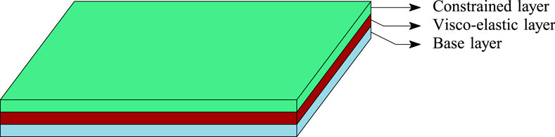
FIGURE 1. Plate structures with constrained-layer damping treatments.
Assuming a baffled plate, the sound pressure at any point can be computed via the Rayleigh integral equation, expressed as Eq. 12:
where pf is the sound pressure, r = |x − y| is the distance between point x and y, k is the wavenumber, and vf is the particle velocity resulting from the structural vibrations. After discretizing by the collocation method, we obtain Eq. 13:
where pf denotes the sound pressure on collocation points, and the particle velocity vf at the collocation points can be interpolated based on the structural displacement u by vf = −vs = iωΘ−1Cfsu, where Θ is the boundary mass matrix [6] and Cfs is the coupling matrix. G is the coefficient matrix, which is dense and asymmetric. Then, the sound power can be computed by the sound pressure and velocity using Eq. 14:
where ()T denotes the transposed matrix. Here, the minus sign is introduced because of the direction of the particle velocity. Z = −GTΘ is the impedance matrix, which is not symmetric due to discretization error when using the collocation method. However, the symmetrization of Z can be simply achieved by Z = (Z + ZT)/2. The Rayleigh integral equation can be regarded as a special case of the BEM, where H = H−1 = I. Considering the symmetry, the sound power can be further rewritten as Eq. 15:
where ZR is the resistive impedance matrix. Another alternation to obtain ZR is first computing the sound power as the integration of sound intensity over the surface Γ, as given in Eq. 16:
Then, as given in Eq. 17, the entry of matrix ZR reads:
If we use a one-point Gauss–Legendre quadrature scheme, the entry can be approximated as given in Eq. 18:
where rij denotes the distance between the collocation points located in elements i and j and Si and Sj are areas of elements i and j. When i = j, r → 0 and (sin kr)/r → k. Apparently, this approach is much more efficient than the collocation method since it does not require integrals. However, this approach cannot yield the sound pressure field because of the singularity in eikr/r.
To omit the cancellation effects of sound intensity, we use NNI proposed by [6] and named by [7] to visualize the surface contribution. Following references [6, 26], sound power can be expressed by Eq. 19:
where
where
where ()H denotes the transpose conjugate of a complex matrix. As proposed by [6], the complex vector β can be calculated by Eq. 22:
where Φ and Λ are the matrix-storing eigenvector ϕ and diagonal matrix-storing eigenvalue λ by solving the following generalized eigenvalue problem, as shown in Eq. 23:
In fact, the computation of the sound power based on β is equivalent to mapping the radiation modes, which could apparently reduce the computational efforts the eigensolutions are truncated, since the radiation is dominated by the first fewer radiation modes in the low-frequency range.
Usually, the objective function of a structural-acoustic system can be categorized into two main types. One is the sound pressure and its variants at one or more points, and the other is the sound power and its variants, which are more suitable for general noise and vibration control in open domains. In this work, we adopt the second type and define the optimization problem as given in Eq. 24:
where the objective function Π represents a real-valued function of state variables u and pf. This expression is adopted for convenience because we will investigate more than one objective function.
Following the SIMP method, elemental matrices can be interpolated as given in Eq. 25:
where μe is the design variable assigned to the eth element and p and q are the penalization factors and are usually chosen to be 3 and 1, respectively. These factors make the intermediate value approach 0 (no visco-elastic element) or 1 (visco-elastic element). Since the damping layer is attached to the base structure, the problem of localized modes can be avoided, as discussed by [27]. Then, the derivatives of the elemental matrices with respect to the eth design variable can be directly given by Eq. 26:
Eq. 26 will be used in the sensitivity analysis.
In the present work, we choose the gradient-based algorithm to solve the optimization problem described in Eq. 24. Hence, the derivative of the objective function, that is, the sensitivity information, is necessary. In the computation of FEM/FMBEM sensitivity, the adjoint variable method (AVM) exhibits excellent accuracy and efficiency [28]. So, AVM is applied for the sensitivity analysis in this work.
First, we can directly write the derivative of the objective function by applying the chain rule as Eq. 27:
where
Then, the direct differentiation of Eq. 11 yields Eq. 29:
Since we only consider design-independent load, the derivative of structural load, that is, ∂fs/∂μe vanishes. Combining Eqs 28 and 29, the derivative of the objective function can be written as Eq. 30:
The derivative of displacement, that is, ∂u/∂μe, is omitted in Eq. 30. By defining the adjoint equation as given in Eq. 31:
and the derivative of the objective function can be finally expressed by the adjoint vector λ as given in Eq. 32:
The adjoint method is therefore not free since it requires solving the extra adjoint equation. The adjoint equation, however, only needs to be solved once because it does not contain derivative components. According to the used interpolation scheme for the material properties defined in Section 3.2, the derivative of the matrix Kd could be simply computed, as given in Eq. 33:
from which, we have Eq. 34:
Since the sound power can be calculated using the sound intensity or NNI, we define two objective functions, as shown in Eq. 35:
where
and Eq. 37 for the objective function PNNI:
Based on the derived
Based on the sensitivity information, the method of moving asymptotes (MMA), see Svanberg [30], is employed to solve the optimization problem. The iteration procedure is repeated until the relative difference of the objective function values in two adjacent iteration steps is less than a prescribed tolerance τ, as shown in Eq. 38:
where Πi denotes the objective function at the ith iteration step. The detailed optimization procedure is presented as follows:
1. Modeling using NURBS. The analyzed structural domain is divided into finite elements, and the impedance matrix and its real part are also computed based on the finite element mesh.
2. Setting up the optimization model with an initial distribution given for the design elements.
3. Solving the response problem described in Eq. 11. Then, the objective function is evaluated based on the solutions u and p. To achieve an efficient reanalysis, we only assemble matrices ZR (and Z) in the first optimization iteration, and these matrices will be recycled in the following iterations.
4. Solving the generalized eigenvalue problem described in Eq. 23 if required, and computing β based on the solution u. Similarly, we also store the eigenvectors and eigenvalues for a possible recycling step.
5. Evaluating the chosen objective function (PSI or PNNI). Then, deriving auxiliary variables
6. Solving the adjoint Eq. 31 for derived
7. When the objective function converges like Eq. 38, optimization is stopped. Otherwise, the design variables are updated using the MMA.
8. Modifying the design variables by the volume-preserving density filter [31], and the procedure is repeated from step 3.
The corresponding flowchart is shown in Figure 2.

FIGURE 2. Flowchart of the detailed optimization procedure.
To investigate the validity and applicability of the developed optimization approach, some numerical examples are performed in this section. All the computations are implemented in an in-house Fortran 95/2003 code. Sparse direct solver PARDISO is applied to all computations involving the global dynamic stiffness Kd. Eigenvalue problems described in Eq. 23 are solved using the ARPACK routines. The convergence tolerance τ in the optimization is set to 10–4.
A baffled plate of dimensions 1 m × 1 m will be chosen as the design object in the following example. It is discretized into 80 × 80 four-node quadrilateral elements, as shown in Figure 3. The finite element model is verified by comparing the natural frequencies and modal loss factors from the present model with those from a closed-form solution [32]. Regarding radiation analysis, the collocation method will be only used when sound intensity is required, otherwise the direct method without integration will be applied instead, in order to save computational costs. We assume the plate to be clamped at its four edges and excited by four harmonic loads F = F0e−iωt as shown in Figure 4. Air is the acoustic medium, with c = 343 m/s and ρ = 1.21 kg/m3. The base and constrained layers consist of aluminum with no damping loss, and the core layer is assumed to consist of a visco-elastic material. Detailed material properties are listed in Table 1.
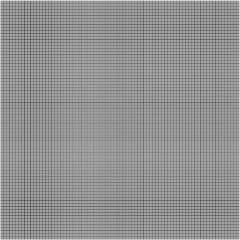
FIGURE 3. Computational grid.
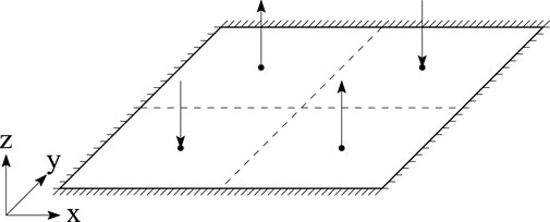
FIGURE 4. Clamped plate example definition.
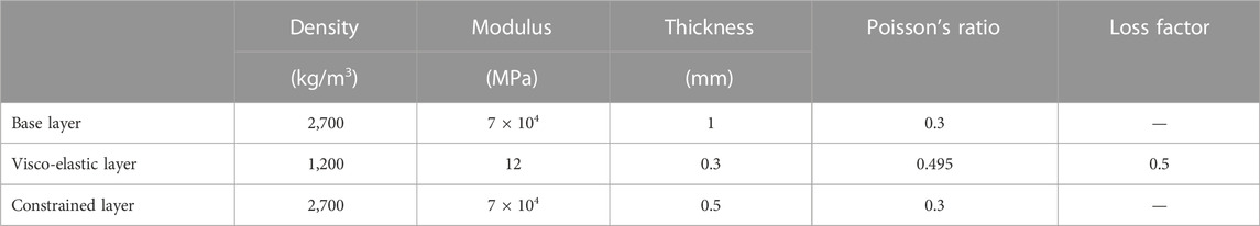
TABLE 1. Material properties of the constrained-layer damping plate.
As mentioned previously, the computational efforts will be reduced when truncating eigensoultions in mapping the radiation modes for evaluating NNI and sound power. Figure 5 shows the Radiated sound power and truncation number versus frequency. In Figure 5A, we compare the sound power computed by sound intensity and NNI resulting from mapping truncated radiation modes, and these two results match very well. We also investigate the truncation number to achieve 99% accuracy compared with the sound power computed by sound intensity in Figure 5B. From the result, we notice that a truncation number of 4 is acceptable for the calculation with a frequency range of 200 Hz. In fact, the sound power is dominantly contributed by the fourth radiation mode because the particle velocity corresponds to the fourth modal pattern. This can be confirmed by investigating the coupling factor of particle velocity with the radiation modes [33]. The coupling factor between the particle velocity pattern and the fourth mode is several orders of magnitude larger than the coupling factor with the first three radiation modes. In the following calculations, we set a higher truncation number of 30 to guarantee correctness and accuracy, and this still saves considerable costs compared with the computation via sound intensity. As a further investigation, we compare the optimization results, which aim at minimizing the radiated computed sound power using truncated acoustic radiation modes. The excitation frequency is assumed to be f = 100 Hz. All the initial design variables are given a uniform value of 1 to avoid possible local minimum. The optimization iteration history is illustrated in Figure 6A. Figures 6B, C show the optimized distributions of the design variables μ. Red (μe = 1) represents the visco-elastic damping element, and blue (μe = 0) indicates that there is no visco-elastic element. Intermediate values (0 < μe < 1) are not physical and are difficult to observe in Figures 6B, C. It can be clearly seen that the two optimizations yield almost the same iteration history and optimization solution. Slight differences between the two optimized designs are possibly caused by numerical error in the eigenvalue analysis and optimization solution. This proves that mapping truncated radiation modes could be an efficient approach to evaluate the sound power without losing accuracy in the response analysis and optimization process at low frequencies. Interestingly, we find that the optimized design yields an even lower sound power (6.6 × 10⁻¹² W) than that (9.7 × 10⁻¹² W) of the initial design with a full visco-elastic damping layer, which is similar to the findings in [29]. This indicates that the investigated optimization is a nonlinear problem and thus stresses the necessity of optimization.
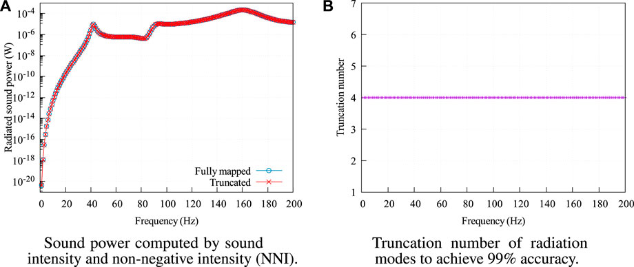
FIGURE 5. Radiated sound power and truncation number versus frequency. (A) Sound power computed by sound intensity and non-negative intensity (NNI). (B) Truncation number of radiation modes to achieve 99% accuracy.
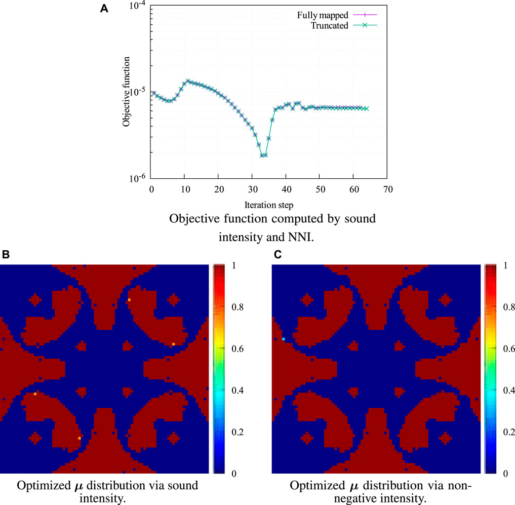
FIGURE 6. Optimization results obtained by sound intensity and NNI. (A) Objective function computed by sound intensity and NNI. (B) Optimized µ distribution via sound intensity. (C) Optimized µ distribution via non-negative intensity.
Figure 7 shows the distributions of sound intensity and NNI, which are different. The result of NNI is consistent with the corner radiation introduced by [34] and confirmed by [5] using the supersonic intensity, while the sound intensity is not consistent since it could be positive or negative. This is similar to the result presented by [6] where the authors used a (1 × 1) structural modal shape as the particle velocity pattern. It has been clearly shown that NNI (computed via mapped radiation modes) could localize the most contributing areas on structural surfaces, while sound intensity fails due to its cancellation effects. But in the aforementioned optimization, NNI does not outperform sound intensity since they give completely the same objective function when the whole surface is selected, that is, the radiated sound power. NNI, however, makes sense if we only want to decrease the radiation contributed by the partial surface. In this case, integration of the sound acoustic intensity, that is, PSI, on the prescribed region does not directly correspond to the intensity that radiates to the far-field. This is the reason why we implement the integration of NNI as the objective function instead of PSI.
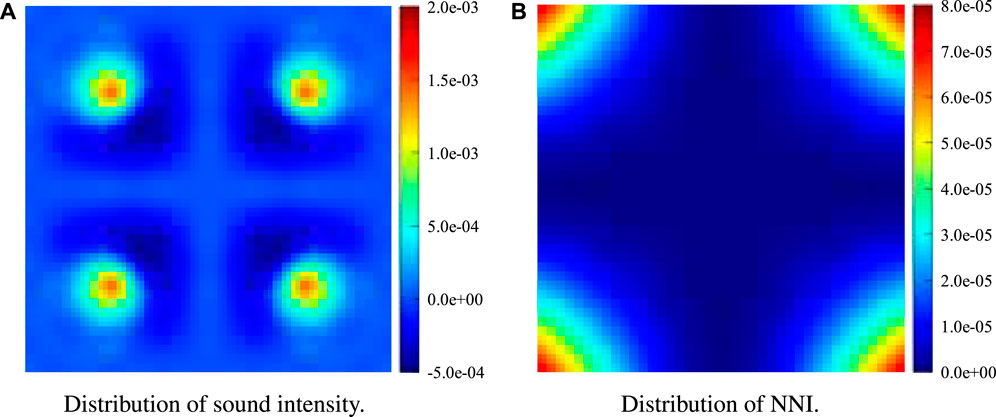
FIGURE 7. Distributions of sound intensity and NNI at 100 Hz. (A) Distribution of sound intensity. (B) Distribution of NNI.
In Figure 8, we split the plate surface into several pieces and choose different pieces as the investigated area Γc where we want to minimize the sound radiation. When choosing the left parts as Γc, the optimization results are obtained and illustrated in Figure 9. The initial values of the design variables are both set to 0.7. From this figure, it can be clearly seen that these two objective functions yield notably different optimized distributions of design variables, as shown in Figures 9A, B. After the optimization, PSI drops from 4.33 × 10⁻⁶ W to −1.18 × 10⁻³ W, while the integration of NNI, that is, PNNI, increases from 4.33 × 10⁻⁶ W to 1.22 × 10⁻³ W. That is to say, the real contributions from the left parts are enlarged by the optimization, which indicates that PSI cannot correspond to the energy radiated to the far-field. By contrast, the optimization minimizing PNNI produces a reduction from 4.33 × 10⁻⁶ W to 2.19 × 10⁻⁶ W. The coincidence between PSI and PNNI at the beginning is due to the symmetry along the y axis with a uniform distribution of design variables. From Figures 9C, D, we notice that the changing tendency of PSI is opposite to that of PNNI, but PNNI and sound power W show a similar tendency. While the contributions from the left parts are considerably decreased, the sound power almost doubles from 8.66 × 10⁻⁶ W to 1.64 × 10⁻⁵ W.
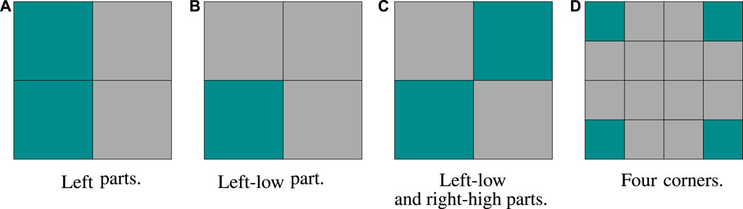
FIGURE 8. Different chosen surface Γc, cyan color represents the chosen parts. (A) Left parts. (B) Lower left part. (C) Lower left and upper right parts. (D) Four corners.
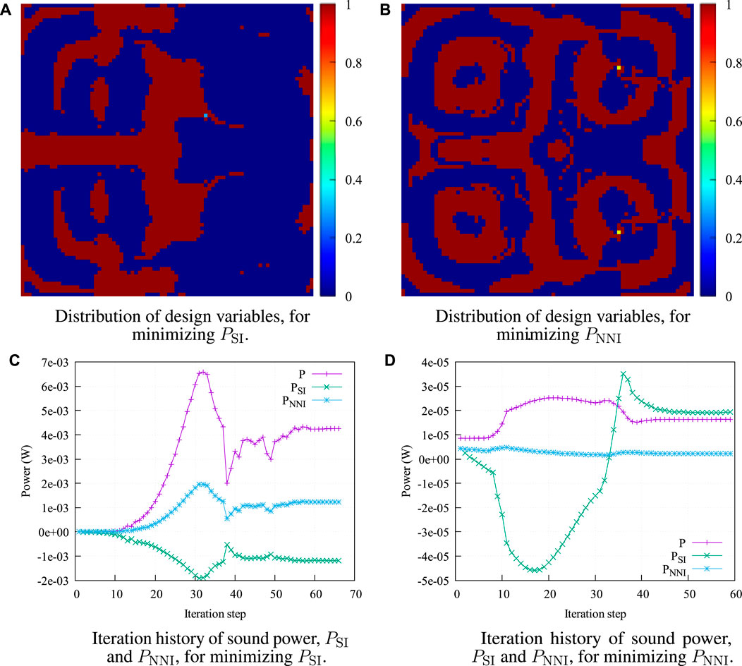
FIGURE 9. Optimization results of PSI and PNNI. The left parts are chosen as the investigated surface Γc. (A) Distribution of design variables, for minimizing PSI. (B) Distribution of design variables, for minimizing PNNI. (C) Iteration history of sound power, PSI and PNNI, for minimizing PSI. (D) Iteration history of sound power, PSI and PNNI, for minimizing PSI.
Figure 10 presents the distributions of sound intensity as well as NNI of the initial design (first row) and two optimized designs (second and third rows). To achieve a better optimization result, we conduct the optimization with different initial values of the design variable: μ = 0.7 and μ = 1 and then show the better one here. This treatment will also be adopted in the following computations. The sound intensity and NNI patterns of the initial design are very similar to those in Figure 7 since they both correspond to a uniform distribution of design variables (μ = 0.7 and μ = 1.0). Hence, homogeneous damping distributions have a very small influence on the patterns of sound intensity and NNI except for detailed values. It is observed the sound intensity and NNI are redistributed by the optimizations in a different manner, which yields inhomogeneous damping distributions. Regarding the sound intensity, there are always adjacent areas exhibiting positive and negative values before and after optimization. From NNI, we notice that two radiating sources located at the left corners become weaker compared with the sources in the right corners after two optimizations. However, compared with the unoptimized source in Figure 10B, the two left sources in Figure 10D correspond to a higher NNI due to improper optimization, with PSI being the objective function. When using PNNI, these two corner sources are successfully suppressed. The optimization makes the contributions from the left corners to the sound power reduce from 50% to approximately 13%. This is attributed to improved cancellation effects of the acoustic source and sink in the left region, and thus less acoustic energy radiates to the far-field. In general, the optimization finally results in an inhomogeneous distribution of structural damping and redistributes the acoustic sink and source accordingly to minimize the objective function. Although the sound intensity performs well when minimizing the sound power is of interest, it shows inferiority in radiation control of the partial or local regions.
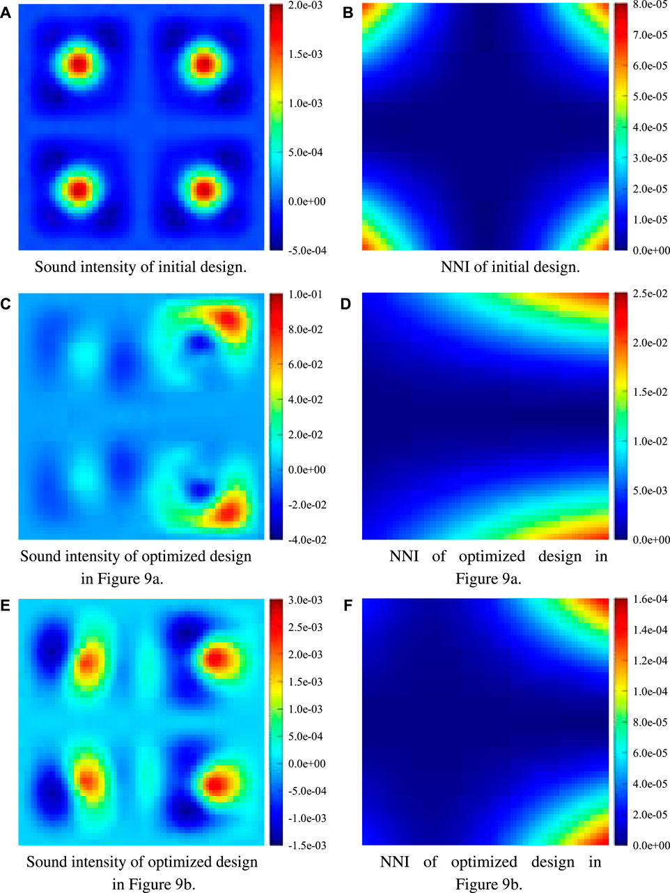
FIGURE 10. Distributions of sound intensity and NNI of different designs. (A) Sound intensity of initial design. (B) NNI of initial design. (C) Sound intensity of optimized design in Figure 9A. (D) NNI of optimized design in Figure 9A. (E) Sound intensity of optimized design in Figure 9B. (F) NNI of optimized design in Figure 9B.
In Table 2, we present the optimization results for different investigated surface Θc, that is, the lower left part. Integrations of the sound intensity and NNI are also selected as the objective function. The first row shows the optimized distributions of design variables μ, resulting from the two objective functions. The second and third rows show the distributions of sound intensity and NNI, and the last row gives the power values before and after optimization. Since the optimization problem is not symmetric along the x and y axes, the resulting designs are also not symmetric anymore. From Table 2, we can see that PSI decreases from 2.2 × 10⁻⁶ W to −5.1 × 10⁻⁴ W, showing a large reduction. PNNI, however, increases from 2.2 × 10⁻⁶ W to 1.4 × 10⁻³ W. Since NNI provides a more accurate visualization of the contribution to sound power, optimization based on PSI becomes meaningless because it increases the radiation from the chosen regions. Furthermore, the contributions from the lower left corner are still higher than those from the upper right corner after optimization aiming to decrease PSI. That is to say, PSI fails to give the desirable contributing/radiation pattern. When optimizing the damping distribution based on PNNI, the power radiated from the predefined region reduces to a very low value of 4.3 × 10⁻⁷ W. The lower left corner becomes the least contributing compared with all other corners, which is exactly as expected. In addition, two corners adjacent to the lower left corner also become inconspicuous due to the redistributed damping. After optimization, there is only one hot spot located in the upper right corner which is opposite to the chosen region. The four-corner radiator becomes a one-corner radiator. Comparing the sound power, we find that all optimized solutions yield a high sound power because the optimization target is not minimizing the sound power radiated from the entire surface. From the sound powers, it can be seen that the increase caused by optimization using PSI can be very large, which is unfavorable. Compared with PSI, the increase in sound power introduced by optimization using PNNI is much smaller.
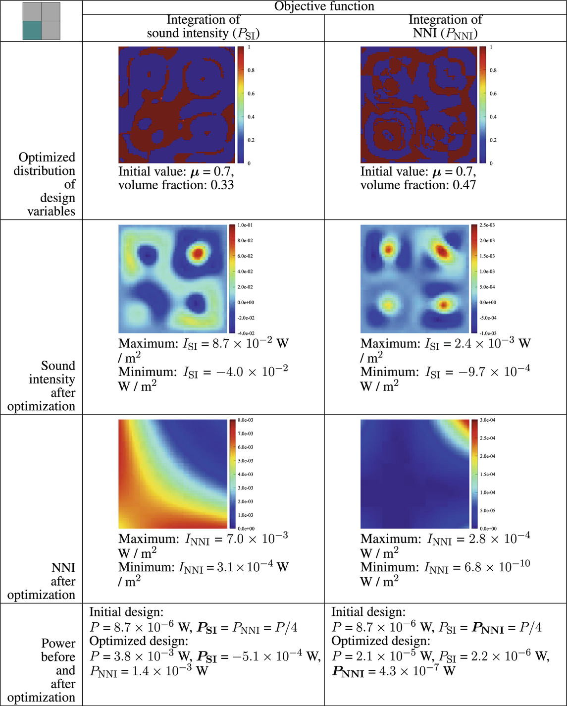
TABLE 2. Optimized results at 100 Hz when the lower left part in Figure 8B is chosen as the investigated surface Γc. The left column corresponds to the results with PSI being the objective function, and the right column corresponds to the results with PNNI being the objective function.
Similar to Tables 2–Tables 4 present optimization results with different investigated surfaces Θc. In Table 3, the lower left and upper right parts are selected. It can be clearly seen that two objective functions generate notably different distributions of the design variables with volume fractions of 0.21 and 0.47, respectively. The four-corner radiator becomes a two-opposite-corner radiator after the two optimizations, minimizing FSI and FNNI, respectively. Because Γc in Figure 8D is symmetric along both the x and y axes, this finally leads to symmetric distributions of damping, as shown in Table 4. We can notice that the distribution of sound intensity and NNI is very similar to that seen in Figure 7, which results from a homogeneous damping distribution. It can be considered that the waves traveling toward high-damped regions (but with opposite directions in one-fourth of the plate area) cancel each other. Hence, the corner mode remains nearly the same as the homogeneous mode. Interestingly, optimization minimizing FSI produces a lower FNNI than optimization aiming at minimizing FNNI. From this aspect, the optimized solution of FNNI is not optimal, indicating that the applied optimization does not make sense. However, we want to stress that this issue is very common in topology optimization for dynamic and acoustic problems since the optimization problem for these investigated systems are highly non-convex. A local optimum is generally reached by the gradient-based algorithm, and it is very hard to get a global optimum. This is the reason why we conduct optimization with different initial values of the design variables, expecting to obtain a good solution (maybe not optimal). Those optimized solutions, however, are generally good designs, which could provide guidance for design and analysis. Thus, choosing a proper initial value for the design variables is of importance for topology optimization. NNI, which could visualize the contributions of the element/region to sound radiation, has the potential to generate a good initial design. Optimization based on this initial design might converge faster than normal initial values, or converge to a better local minimum. This will be investigated in future work.
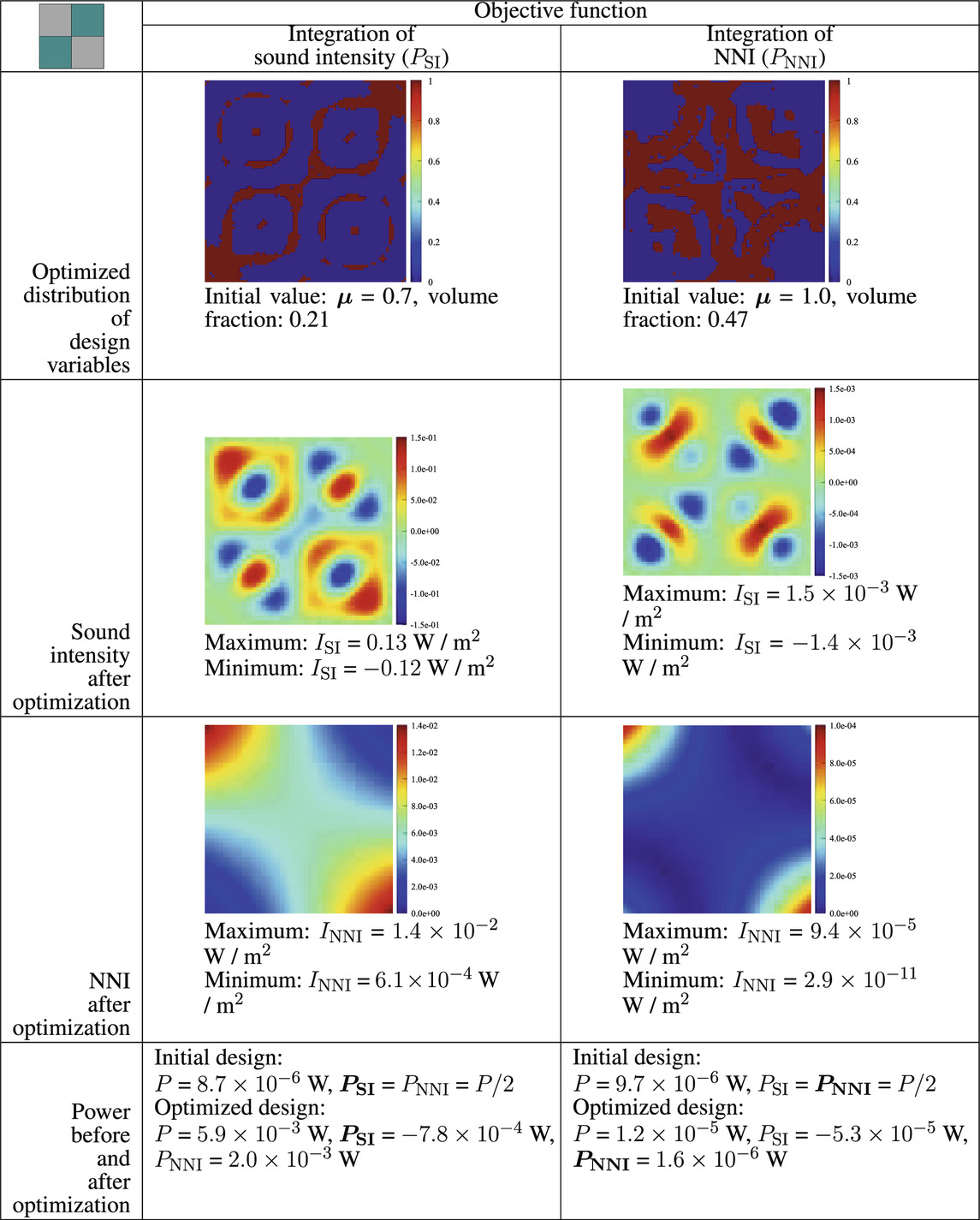
TABLE 3. Optimized results at 100 Hz when the lower left and upper right parts in Figure 8C are chosen as the investigated surface Γc. The left column corresponds to the results with PSI being the objective function, and the right column corresponds to the results with PNNI being the objective function.
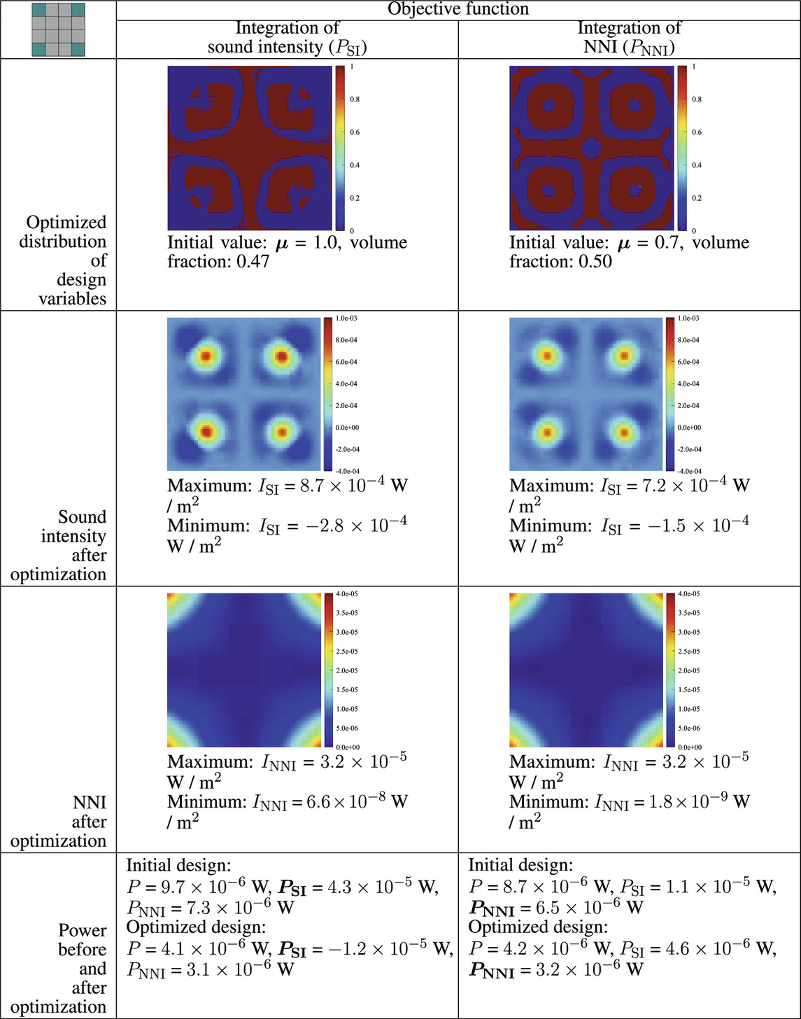
TABLE 4. Optimized results at 100 Hz when the four corners in Figure 8D are chosen as the investigated surface Γc. The left column corresponds to the results with PSI being the objective function, and the right column corresponds to the results with PNNI being the objective function.
From the results discussed previously, it can be clearly seen that the radiation pattern is optimized by using predefined objective functions. Optimized designs usually show higher sound powers than unoptimized designs. However, the increases in sound power caused by optimization using FNNI are not usually very large and can sometimes be acceptable if the sound power is not of high importance. This is attributed to how we select regions with high contributions to sound radiation as the investigated area Γc, such as the corners of the plate. This is reasonable because these regions are always of greater interest compared with other less contributing areas. In contrast, optimization possibly produces a sound power several orders of magnitude larger when choosing FSI as the objective function. Such enormous increases are usually unfavorable in engineering. Hence, it is not recommended to optimize the radiation pattern based on the integration of sound intensity.
Finally, we have to admit that the physical meanings of NNI are still unclear, and further research on NNI is required. However, it can be clearly seen that optimization using NNI has the potential to optimize the radiating pattern and outperforms the sound intensity in designing the radiation pattern.
An approach to optimizing the contributing pattern to radiated sound power from vibrating structures has been introduced. Two different predefined objective functions, namely, the integrations of NNI and sound intensity over chosen surfaces, are applied and compared in the optimization. By using these objective functions, an optimized damping layer distribution can be found which reduces the contribution to the sound power from the surfaces of interest. When the entire surface is of interest, these two objective functions are equivalent to the radiated sound power, and two optimizations give almost the same result. However, NNI can be extracted from truncated radiation modes, and usually requires less computational effort than sound intensity. This could improve the computational efficiency of optimization. When only partial surfaces are of interest, two predefined objective functions produce quite different optimized designs. However, optimization using the sound intensity possibly yields an enormous increase in the radiated sound power, which is usually unfavorable in engineering designs. Furthermore, it sometimes fails to generate a desirable radiating pattern. In contrast, optimization using NNI always leads to a desirable radiating pattern with only a slightly increased sound power. Thus, we strongly recommend using NNI to optimize the radiating/contributing pattern. The optimization procedure presented here provides a new way for radiating pattern control.
The original contributions presented in the study are included in the article/Supplementary Material; further inquiries can be directed to the corresponding author.
Conceptualization, YX; data curation, XZ; formal analysis, XZ; investigation, XZ; methodology, YX; project administration, YX; software, XZ; supervision, YX; validation, XZ; visualization, XZ; and writing—original draft, XZ and YX. All authors have read and agreed to the published version of the manuscript.
The authors declare that the research was conducted in the absence of any commercial or financial relationships that could be construed as a potential conflict of interest.
All claims expressed in this article are solely those of the authors and do not necessarily represent those of their affiliated organizations, or those of the publisher, the editors, and the reviewers. Any product that may be evaluated in this article, or claim that may be made by its manufacturer, are not guaranteed or endorsed by the publisher.
1. Bendsøe MP, Kikuchi N. Generating optimal topologies in structural design using a homogenization method. Comp Methods Appl Mech Eng (1988) 71:197–224. doi:10.1016/0045-7825(88)90086-2
2. Du J, Olhoff N. Minimization of sound radiation from vibrating bi-material structures using topology optimization. Struct Multidisc Optim (2007) 33:305–21. doi:10.1007/s00158-006-0088-9
3. Xu Z, Huang Q, Zhao Z. Topology optimization of composite material plate with respect to sound radiation. Eng Anal Boundary Elem (2011) 35:61–7. doi:10.1016/j.enganabound.2010.05.013
4. Zheng W, Yang T, Huang Q, He Z. Topology optimization of PCLD on plates for minimizing sound radiation at low frequency resonance. Struct Multidisc Optim (2015) 53:1231–42. doi:10.1007/s00158-015-1371-4
5. Williams EG. Supersonic acoustic intensity on planar sources. The J Acoust Soc America (1998) 104:2845–50. doi:10.1121/1.423868
6. Marburg S, Lösche E, Peters H, Kessissoglou N. Surface contributions to radiated sound power. J Acoust Soc America (2013) 133:3700–5. doi:10.1121/1.4802741
7. Williams EG. Convolution formulations for non-negative intensity. J Acoust Soc America (2013) 134:1055–66. doi:10.1121/1.4812262
8. Liu D, Peters H, Marburg S, Kessissoglou N. Supersonic intensity and non-negative intensity for prediction of radiated sound. J Acoust Soc America (2016) 139:2797–806. doi:10.1121/1.4948567
9. Hughes TJ, Cottrell JA, Bazilevs Y. Isogeometric analysis: CAD, finite elements, NURBS, exact geometry and mesh refinement. Comp Methods Appl Mech Eng (2005) 194:4135–95. doi:10.1016/j.cma.2004.10.008
10. Gu J, Zhang J, Li G. Isogeometric analysis in BIE for 3-D potential problem. Eng Anal Boundary Elem (2012) 36:858–65. doi:10.1016/j.enganabound.2011.09.018
11. Zang Q, Liu J, Ye W, Lin G. Isogeometric boundary element method for steady-state heat transfer with concentrated/surface heat sources. Eng Anal Boundary Elem (2021) 122:202–13. doi:10.1016/j.enganabound.2020.11.001
12. Ibáñez MJ, Barrera D, Maldonado D, Yáñez R, Roldán JB. Non-uniform spline quasi-interpolation to extract the series resistance in resistive switching memristors for compact modeling purposes. Mathematics (2021) 9:2159. doi:10.3390/math9172159
13. Wang L, Xiong C, Yuan X, Wu H. Discontinuous galerkin isogeometric analysis of convection problem on surface. Mathematics (2021) 9:497. doi:10.3390/math9050497
14. Yu B, Cao G, Huo W, Zhou H, Atroshchenko E. Isogeometric dual reciprocity boundary element method for solving transient heat conduction problems with heat sources. J Comput Appl Math (2021) 385:113197. doi:10.1016/j.cam.2020.113197
15. Yu B, Cao G, Meng Z, Gong Y, Dong C. Three-dimensional transient heat conduction problems in FGMs via IG-DRBEM. Comp Methods Appl Mech Eng (2021) 384:113958. doi:10.1016/j.cma.2021.113958
16. Chen L, Lian H, Liu Z, Gong Y, Zheng C, Bordas S. Bi-material topology optimization for fully coupled structural-acoustic systems with isogeometric FEM-BEM. Eng Anal Boundary Elem (2022) 135:182–95. doi:10.1016/j.enganabound.2021.11.005
17. Chen L, Lian H, Natarajan S, Zhao W, Chen X, Bordas S. Multi-frequency acoustic topology optimization of sound-absorption materials with isogeometric boundary element methods accelerated by frequency-decoupling and model order reduction techniques. Comp Methods Appl Mech Eng (2022) 395:114997. doi:10.1016/j.cma.2022.114997
18. Peng X, Lian H, Ma Z, Zheng C. Intrinsic extended isogeometric analysis with emphasis on capturing high gradients or singularities. Eng Anal Boundary Elem (2022) 134:231–40. doi:10.1016/j.enganabound.2021.09.022
19. Chen L, Lian H, Xu Y, Li S, Liu Z, Atroshchenko E, et al. Generalized isogeometric boundary element method for uncertainty analysis of time-harmonic wave propagation in infinite domains. Appl Math Model (2023) 114:360–78. doi:10.1016/j.apm.2022.09.030
20. Chen L, Lian H, Liu Z, Chen H, Atroshchenko E, Bordas S. Structural shape optimization of three dimensional acoustic problems with isogeometric boundary element methods. Comp Methods Appl Mech Eng (2019) 355:926–51. doi:10.1016/j.cma.2019.06.012
21. Peng X, Atroshchenko E, Kerfriden P, Bordas S. Isogeometric boundary element methods for three dimensional static fracture and fatigue crack growth. Comp Methods Appl Mech Eng (2017) 316:151–85. doi:10.1016/j.cma.2016.05.038
22. Peng X, Atroshchenko E, Kerfriden P, Bordas S. Linear elastic fracture simulation directly from CAD: 2D NURBS-based implementation and role of tip enrichment. Int J Fract (2017) 204:55–78. doi:10.1007/s10704-016-0153-3
23. Keuchel S, Hagelstein NC, Zaleski O, von Estorff O. Evaluation of hypersingular and nearly singular integrals in the Isogeometric Boundary Element Method for acoustics. Comp Methods Appl Mech Eng (2017) 325:488–504. doi:10.1016/j.cma.2017.07.025
24. Nguyen VP, Anitescu C, Bordas SP, Rabczuk T. Isogeometric analysis: An overview and computer implementation aspects. Mathematics Comput Simulation (2015) 117:89–116. doi:10.1016/j.matcom.2015.05.008
25. Zheng L, Xie R, Wang Y, Adel E-S. Topology optimization of constrained layer damping on plates using method of moving asymptote (MMA) approach. Shock and Vibration (2011) 18:221–44. doi:10.1155/2011/830793
26. Wilkes DR, Peters H, Croaker P, Marburg S, Duncan AJ, Kessissoglou N. Non-negative intensity for coupled fluid-structure interaction problems using the fast multipole method. J Acoust Soc America (2017) 141:4278–88. doi:10.1121/1.4983686
27. Olhoff N, Du J. Generalized incremental frequency method for topological design of continuum structures for minimum dynamic compliance subject to forced vibration at a prescribed low or high value of the excitation frequency. Struct Multidisc Optim (2016) 54:1113–41. doi:10.1007/s00158-016-1574-3
28. Chen L, Marburg S, Chen H, Zhang H, Gao H. An adjoint operator approach for sensitivity analysis of radiated sound power in fully coupled structural-acoustic systems. J Comp Acous (2017) 25:1750003. doi:10.1142/s0218396x17500035
29. Zhao W, Zheng C, Chen H. Acoustic topology optimization of porous material distribution based on an adjoint variable FMBEM sensitivity analysis. Eng Anal Boundary Elem (2019) 99:60–75. doi:10.1016/j.enganabound.2018.11.003
30. Svanberg K. The method of moving asymptotes—A new method for structural optimization. Int J Numer Meth Engng (1987) 24:359–73. doi:10.1002/nme.1620240207
31. Xu S, Cai Y, Cheng G. Volume preserving nonlinear density filter based on heaviside functions. Struct Multidisc Optim (2010) 41:495–505. doi:10.1007/s00158-009-0452-7
32. Johnson CD, Kienholz DA. Finite element prediction of damping in structures with constrained viscoelastic layers. AIAA J (1982) 20:1284–90. doi:10.2514/3.51190
33. Unruh O. Influence of inhomogeneous damping distribution on sound radiation properties of complex vibration modes in rectangular plates. J Sound Vibration (2016) 377:169–84. doi:10.1016/j.jsv.2016.05.009
Keywords: topology optimization, constrained-layer damping, non-negative intensity, sound radiation, isogeometric analysis
Citation: Zhang X and Xu Y (2023) Design of constrained-layer damping on plates to sound radiation based on isogeometric analysis and non-negative intensity. Front. Phys. 10:1072230. doi: 10.3389/fphy.2022.1072230
Received: 17 October 2022; Accepted: 08 November 2022;
Published: 10 January 2023.
Edited by:
Pei Li, Xi’an Jiaotong University, ChinaReviewed by:
Haojie Lian, Taiyuan University of Technology, ChinaCopyright © 2023 Zhang and Xu. This is an open-access article distributed under the terms of the Creative Commons Attribution License (CC BY). The use, distribution or reproduction in other forums is permitted, provided the original author(s) and the copyright owner(s) are credited and that the original publication in this journal is cited, in accordance with accepted academic practice. No use, distribution or reproduction is permitted which does not comply with these terms.
*Correspondence: Yanming Xu, eHV5YW5taW5nQHVzdGMuZWR1
Disclaimer: All claims expressed in this article are solely those of the authors and do not necessarily represent those of their affiliated organizations, or those of the publisher, the editors and the reviewers. Any product that may be evaluated in this article or claim that may be made by its manufacturer is not guaranteed or endorsed by the publisher.
Research integrity at Frontiers
Learn more about the work of our research integrity team to safeguard the quality of each article we publish.