Financial crisis prediction based on multilayer supervised network analysis

Financial crisis prediction is essential in preventing financial problems as its monitoring indicators help regulators judge the probability of future crises. In this context, the activities of the scientific community have been focused on the dynamics of single/multiple sequences and utilized unsupervised/supervised methods for financial crisis prediction. It is noteworthy that the cross-correlation between the risks of multiple economic entities makes financial network analysis paramount in crisis prediction. Focusing on this point, we propose a multilayer supervised network analysis (MSNA) method to train the multilayer network, and select the most suitable layer for financial crisis prediction. Specifically, we use 37 crucial stock market indices from 4 continents to create successive multilayer financial networks with 120-day windows and 1-day step by Pearson cross-correlation (PCC), variance decompositions (VD), transfer entropy (TE), minimum spanning tree (MST), directed MST (DMST), planar maximally filtered graph (PMFG) and directed PMFG (DPMFG) methods. Based on the multilayer network, we embed the graph neural network classification (GNNC) model and train the dynamic multilayer networks at each window scale (240,120, and 60 days). Finally, we conclude that the accuracy of the short window (60 days) is significantly higher than that of the long window. The network constructed by PCC with MST is the most suitable for short sequence (60 days) crisis prediction (AUC = 0.959), and the network constructed by TE with DMST is the most suitable for long sequence (240 days) crisis prediction (AUC = 0.772).

1 Introduction

A financial crisis refers to various situations, such as stock market crashes and bursting of financial bubbles, in which some financial assets suddenly lose a large part of their nominal value. Many economists have proposed theories about how financial crises develop and how they can be prevented. Frankel and Rose predicted the probability of crises by establishing the joint probability distribution between independent and dependent variables [1]. Subsequently, Kaminsky et al.used the KLR signal analysis method to detect the index signals exceeding the threshold at a certain time point or period, and used signal strength for crisis prediction [2]. Further, Berg et al. integrated the advantages of the FR probability model and KLR signal analysis method and created DCSD (developing country studies division) model, that can send out early warning signals for crises more accurately and shorten the prediction interval to 24 months [3]. However, the probability model, the KLR signal analysis method and DCSD model do not consider the heterogeneity of the financial crisis and the difference in the actual situation between countries. Sachs et al. constructed an STV cross-sectional model of a currency crisis early warning system based on cross-sectional data [4].

Some scholars have constructed quantitative indices for financial crisis prediction. Billio et al. used an entropy measure to analyze the evolution of systemic risk among European banks and constructed a banking crisis early warning index system based on marginal expected shortfall (MES), conditional value at risk (CoVaR) indicators and network connectivity. Additionally, they determine the effectiveness of entropy measures in banking crisis prediction [5]. Dastkha et al. used CoVaR as a market-based systematic risk measurement method to investigate the systematic risk of the Tehran stock exchange and provide early warning signals of systematic risk [6].

As the FR probability model, KLR signal, and risk quantitative index can only explain the occurrence of crisis and cannot compare and test the early-warning results, Kumar et al. established a logit model to test the effects of early crisis warnings [7]. Moreover, Klomp used a random coefficient logit model to improve the traditional logit model and analyzed the heterogeneity of banking crises from 1970 to 2007 [8]. Schularick et al. used a logit model for crisis prediction and proved that credit growth is a powerful predictor of financial crisis [9]. Similarly, Greenwood et al. posited that crises can be predicted using past credit growth in simple linear forecasting regressions, and that the probability of a financial crisis within the next 3 years is 45% [10]. Boonman et al. applied the KLR Signal method and logit model method to the data of 15 groups of emerging economies, and found that the index prediction based on consistent expectation tended to eliminate extreme situations, resulting in no timely warning when predicting a large number of crises [11]. This shows that the logit prediction model can determine the key leading indicators of the financial crisis. Moreover, some important indicators lead to false early warnings. Simultaneously, the prediction time of the logit model for a crisis remains at 24 months.

To enhance the prediction accuracy of limited data, Sornette et al. used the log-periodic power law singularity (LPPLS) method to evaluate data on the Shanghai and Shenzhen stock indices from May 2005 to July 2009. The results show that the LPPLS method can successfully find the prediction signals before the two-stage sharp decline in China’s stock market (from mid-2005 to October 2007, and from November 2008 to early August 2009), and improve the prediction accuracy to approximately 2 months [12]. Fricke used a machine learning model and a traditional logit model to predict various financial crises and discovered that the prediction results of the machine learning model were not always more accurate than those of the traditional logit model [13]. Tölö used long-term and short-term memory (RNN-LSTM) and gated recursive unit (GRU) neural network model for crisis prediction. They found that the prediction effect of the RNN-LSTM method was significantly higher than that of the traditional logit model [14]. Zhu et al. used a K-means clustering algorithm to classify financial risk types and optimize the financial risk control. They found that the K-means algorithm can distinguish the state intervals of different financial crises more accurately and objectively [15]. Liu et al. found that the machine learning models, especially the random forest, gradient boosting decision tree, and ensemble models, outperform logistic models in terms of providing early predictions of financial crises [16].

Nevertheless, LPPLS method and machine learning model generally utilize a single stock for prediction, lack consideration of the correlation analysis between multiple financial institutions, and can not investigate the risk contagion of financial institutions. The question that needs to be considered is as follows: How can the correlation of financial markets be applied to crisis prediction and improve supervised characteristics?

Due to the complexity of the financial system and the unrealistic theoretical assumptions, it is difficult to provide scientific and effective suggestions for economic policies after the financial crisis, and to point out the need to studying financial problems from the perspective of a complex system [17–20]. As an emerging technical means, the financial complex network is very intuitive in describing the relationship of various financial elements. Building an effective financial network has always been the focus of scholars’ researchers worldwide. In recent years, many methods have been used to build a financial network. Researchers have used Pearson cross-correlation [21], mutual information [22], Granger causality tests [23, 24], transfer entropy [25] and variance decomposition [26]to create financial matrices expressing the relationship between financial institutions. Additionally, they have used the threshold method [27], MST method [28, 29], plane maximum filter graph method [30], DMST [31] and DPMFG [32] to create financial networks. However, a problem that still needs to be considered is how to build a network that is suitable for financial crisis prediction. Hence, it is necessary to use the crisis prediction results as a supervised condition for the supervision and early warning analysis of high-dimensional financial networks.

Traditional machine learning and neural network models [33–36] have limitations when processing non-Euclidean spatial data (e.g., financial networks, social networks and information networks). In addition, compared with the most basic network structure of neural network containing the total connection layer (MLP), the graph neural network [37, 38] has an adjacency matrix, which simplifies the calculation form and improves the calculation efficiency.

With the help of the excellent performance of graph neural network method in graph classification, we integrate multilayer network construction method and graph neural network supervised analysis to study the supervision and prediction of financial crisis. The method derived from this paper is called multi-layer supervised network analysis (MSNA). Specifically, we constructed multilayer networks by utilizing PCC, VD and TE combining with MST and PMFG. We employed the graph neural network classification method to add the supervised characteristics to the multilayer networks, and use the existing crises as the tag values to study the supervision and financial crisis prediction.

The remainder of this paper is organized as follows. In Section 2, we present our method (i.e.,MSNA) of the article in two parts: 1) the construction of the multiplex network and, 2) the supervised characteristics of dynamic multiplex networks. In Section 3, our datasets are briefly presented. In Section 4, we show the main results. The findings show that the MSNA model has better prediction results, compared with long series. Second, the first-layer network (PCC-MST) is the most suitable for financial crisis prediction. Section 5 presents the conclusions and discussion.

2 Materials and methods

2.1 Multiplex network creation

2.1.1 Creating a pearson correlation-coefficient network

The complex relationships between stocks vary with the stock market and the economic environment. Thus we can use these relationships to describe the state of the stock market. We consider many stock log-return series, and each index is as follows:

$P=\left\{\begin{array}{cccc}\hfill P_{\mathrm{1,1}}\hfill & \hfill P_{\mathrm{1,2}}\hfill & \hfill \cdots \hfill & \hfill P_{1,T+1}\hfill \\ \hfill P_{\mathrm{2,1}}\hfill & \hfill \ddots \hfill & \hfill \cdots \hfill & \hfill P_{2,T+1}\hfill \\ \hfill ⋮\hfill & \hfill ⋮\hfill & \hfill \ddots \hfill & \hfill ⋮\hfill \\ \hfill P_{M,1}\hfill & \hfill P_{M,2}\hfill & \hfill \cdots \hfill & \hfill P_{M,T+1}\hfill \end{array}\right\}(1)$

where P_i,t is the price of the index i on day t. We calculate the daily return for each index i as:

$\begin{array}{c}R=\left\{r_{i,t+1}\equiv \ln P_{i,t+1}-\ln P_{i,t},\right.\hfill \\ \left.i=\mathrm{1,2},,\dots ,M;t=\mathrm{1,2},\dots ,T.\right\}\hfill \end{array}(2)$

where T denotes the total length of the stock log-return series, M indecates the number of the log-return series. A series of sequence fragments is extracted from the sequences R by a sliding window whose length is L.

$\begin{array}{l}\hfill \begin{array}{cc}\hfill R_s& =\left\{\begin{array}{cccc}\hfill r_{1,\mathrm{\Delta }\blacksquare \left(s-1\right)+1}\hfill & \hfill r_{1,\mathrm{\Delta }\blacksquare \left(s-1\right)+2}\hfill & \hfill \cdots \hfill & \hfill r_{1,\mathrm{\Delta }\blacksquare \left(s-1\right)+L}\hfill \\ \hfill r_{2,\mathrm{\Delta }\blacksquare \left(s-1\right)+1}\hfill & \hfill \ddots \hfill & \hfill \cdots \hfill & \hfill r_{2,\mathrm{\Delta }\blacksquare \left(s-1\right)+L}\hfill \\ \hfill ⋮\hfill & \hfill ⋮\hfill & \hfill \ddots \hfill & \hfill ⋮\hfill \\ \hfill r_{M,\mathrm{\Delta }\blacksquare \left(s-1\right)+1}\hfill & \hfill r_{M,\mathrm{\Delta }\blacksquare \left(s-1\right)+2}\hfill & \hfill \cdots \hfill & \hfill r_{M,\mathrm{\Delta }\blacksquare \left(s-1\right)+L}\hfill \end{array}\right\}\text{\hspace{0.17em},}\hfill \\ \hfill s& =\mathrm{1,2},\cdots W,W=\left[\frac{T-L}{\mathrm{\Delta }}\right]+1\hfill \end{array}\end{array}(3)$

where Δ denotes the sliding step and W indicates the total number of fragments, [.] means rounding. The sth segment of R, R_s, and Pearson correlations between stocks are as follows:

$\begin{array}{l}\hfill \begin{array}{cc}\hfill {\rho }_{i,j}\left(s\right)& =\frac{\sum _{t=1}^L\left(r_{i,\mathrm{\Delta }\blacksquare \left(s-1\right)+t}-\overline{R_s\left(i,.\right)}\right)\left(r_{j,\mathrm{\Delta }\blacksquare \left(s-1\right)+t}-\overline{R_s\left(j,.\right)}\right)}{\sqrt{\sum _{t=1}^L{\left(r_{i,\mathrm{\Delta }\blacksquare \left(s-1\right)+t}-\overline{R_s\left(i,.\right)}\right)}^2}\blacksquare \sqrt{\sum _{t=1}^L{\left(r_{j,\mathrm{\Delta }\blacksquare \left(s-1\right)+t}-\overline{R_s\left(j,.\right)}\right)}^2}},\hfill \\ \hfill s& =\mathrm{1,2},\cdots W,i=\mathrm{1,2},\cdots M,j=\mathrm{1,2},\cdots M.\hfill \end{array}\end{array}(4)$

where Eq. 4 represents the correlation coefficient of two sequences of the s fragments, while $\overline{R_{s,i}}$ and $\overline{R_{s,j}}$ represents the average value of the i row and j row in formula Eq. 3 respectively.

For these Pearson correlation matrices, we choose two popular methods (MST and PMFG) to create financial networks. The steps of the Kruskal MST method are as follows:

1) Translate the Pearson correlation matrix to a distance matrix:

$D_{ij}=\sqrt{2\left(1-{\rho }_{ij}\right)}(5)$

where D_ij indicates the distance between stock i and stock j,

2) Sort the values from the distance matrix named $D_{ij}^{ac}$ in ascending order.

3) Add the edge to the spanning tree from $D_{ij}^{ac}$ in ascending order. If the adding edge forms a ring, we select the next value in $D_{ij}^{ac}$ and skip this edge.

4) Repeat step 3 until the number of edges is M − 1.

The simplest structure can be obtained from the MST, but some important information is ignored. Thus we also use the PMFG method to create a network using a Pearson correlation matrix. The steps of the PMFG method are as follows:

1) The correlation degree between each node is arranged in ascending order according to the values in the matrix.

2) The corresponding node pairs are selected from the arranged weight values in order to establish the edge connection. If the newly added edge makes the network appear non-planar, that is, if the newly added edge and its other edges cross on a plane, the connection will be abandoned.

3) Repeat step 2 until all nodes join the network.

In this way, we constructed the dynamic Pearson correlation matrices into multilayer networks using the MST and PMFG method. The two networks are regarded as first-layer (PCC-MST) and second-layer (PCC-PMFG) networks.

2.1.2 Construction of a risk spillover network

Although the Pearson correlation network can analyze the volatility correlation between stocks, it can not explain the risk spillover between stocks. Therefore, we intend to use the VD method to create a risk spillover network. The steps of the VD method [26] are as follows:

1) We construct A VAR(Q) process (1) model based on the relevant infectious variables of financial institutions to establish inter-agency relationships as follows:

$z_t=\sum _{q=1}^Q{\varphi }_q{z}_{t-q}+{\epsilon }_t(6)$

$z_t=\sum _{q=0}^{\infty }{A}_q{\epsilon }_{t-q}(7)$

where z_t is a M-dimensional vector of endogenous variables. A_q is a M-by-M matrix, ϕ represents the parameter matrix, ɛ indicates independent and identically distributed perturbed term and follows: ɛ ∼ (0, ∑). The forms of Aq in Eq. 7 are as follows:

$A_q={\varphi }_1{A}_{q-1}+{\varphi }_2{A}_{q-2}+\cdots +{\varphi }_p{A}_{q-Q}(8)$

where A₀ is a unit matrix and A₀ = 0 when q < 0.

2) Based on Eqs 6–8, we obtain the directed correlation coefficients between mechanisms in different periods (forward H step) using the generalized variance decomposition technique. The calculation formulas are as follows:

$d_{ij}^h=\frac{{\sigma }_{ii}^{-1}\sum _{h=0}^{H-1}{\left({e^{\prime }}_i{A}_h{\sum e}_j\right)}^2}{\sum _{h=0}^{H-1}{\left({e^{\prime }}_i{A}_h{\sum {A^{\prime }}_{h}e}_i\right)}^2}(9)$

where Σ is the covariance matrix of the error ɛ, σ_ii is the standard deviation of error for the ith equation. Further, e_j is a selection vector with jth element unity and zeros elsewhere. Additionally, $d_{ij}^h$ is called directed spillover index of j over i. Lastly, H indicates the number of steps to forward the predicted variance.

The risk spillover network created directly by the directed spillover matrix contains many noise edges. We intend to use DMST and DPMFG to reduce the noise and create multilayer financial networks namely, third-layer (VD-DMST) and fourth-layer (VD-DPMFG) networks. The steps of DMST [39] are as follows:

1) Select a node as the root node randomly.

2) Travel all edges and find the smallest entry edges of all points except for the root node. Then, the weighted values of the edges are summed to form a new graph. The final minimum arborescence is determined if no cycles exist in the new graph.

3) If a ring exists in the new graph, it shrinks the ring into a point and change the edge weight. The steps to change the edge weights are as follows:

① Choose a node u in the ring and set the incoming edge of this node as in [u], and the outgoing edge of this node as (u, i, w). Further, i and w refer to the source node and the weight, respectively. ② Set the new edge weight of node u as (u, i, w − in [u]). ③ Return to Step 2 if the new weight graph contains rings.

4) Expand the new graph if rings do not exist by the breaking loop method [40]. The steps of the breaking loop method are as follows:

① Find a loop in the graph. ② Remove the edge with the largest weight in the loop, but keep the graph connected. ③ Repeat this process until there are no loops in the graph (but they are still connected) and get the minimum spanning tree.

The steps of DPMFG [32] are as follows:

1) We convert the asymmetric matrix into a symmetric matrix by summing two edges.

2) We use PMFG to transfer the symmetric matrix into a PMFG matrix.

3) Based on the result of the PMFG matrix, we select the larger of the two edges to represent the direction and delete the smaller one.

2.1.3 Constructing information transmission networks

The risk spillover network can describe the contagion from one stock to others, but cannot describe the co-movement between stocks. Thus we select transfer entropy to express the co-movement and information transmission between stocks. Transfer entropy [41] developed by Schreiber is a measure to evaluate dynamic, nonlinear, and non-symmetric relationships. The measurement of Transfer Entropy is Shannon Entropy. Shannon Entropy is defined as follows:

$E=-\sum _{t=1}^N{p}_t\log p_t,(10)$

for a sequence x and p_t ≠ 0, where N is the number of bins by dividing the sequence x, p_t is the probability of the tth bin by the probability density function (PDF). Based on Shannon entropy, transfer entropy can be conceived as a parameter that can be used for describing the interaction between the series X and Y. Reciprocities have directivity, TE_x→y or TE_y→x. The transition probabilities can be defined as follows:

$p\left(x_{t+1}\mid x_t^{\left(k\right)},y_t^{\left(l\right)}\right)=p\left(X_{t+1}=x_{t+1}\mid X_t^{\left(k\right)}=x_t^{\left(k\right)},Y_t^{\left(l\right)}=y_t^{\left(l\right)}\right)(11)$

where time series of X could be treated as a Markov process of degree k. Likewise, Y is l degree Markov process. $X_t^{(k)}=(X_t,X_{t-1},\dots ,X_{t-k+1})$ and $Y_t^{(l)}=(Y_t,Y_{t-1},\dots ,Y_{t-l+1})$. $x_t^{(k)}$ and $y_t^{(k)}$ are the states of $X_i^{(k)}$ and $Y_i^{(l)}$, respectively. The transfer entropy from one variable Y to the other variable X is defined as follows:

$\begin{array}{ll}\hfill T{E}_{Y\to X}\left(k,l\right)& =E\left(X_{t+1}\mid X_t^{\left(k\right)}\right)-E\left(X_{t+1}\mid X_t^{\left(k\right)},Y_t^{\left(l\right)}\right)\hfill \\ \hfill & =\sum p\left(x_{t+1},x_t^{\left(k\right)},y_t^{\left(l\right)}\right)\log \frac{p\left(x_{t+1}\mid x_t^{\left(k\right)},y_t^{\left(l\right)}\right)}{p\left(x_{t+1}\mid x_t^{\left(k\right)}\right)}\hfill \\ \hfill & =\sum _{i_{t+1},i_t^{\left(k\right)},j_n^{\left(l\right)}}p\left(i_{t+1},i_t^{\left(k\right)},j_t^{\left(l\right)}\right)\log \frac{p\left(i_{t+1},i_t^{\left(k\right)},j_t^{\left(l\right)}\right)p\left(i_t^{\left(k\right)}\right)}{p\left(i_{t+1},i_t^{\left(l\right)}\right)p\left(i_t^{\left(k\right)},j_t^{\left(l\right)}\right)}\hfill \end{array}(12)$

where i_t is element t of the time series of variable X and j_t is element t of the time series of variable Y. To facilitate the calculation of transfer entropy, we take k = l = 1. Thus the normal formula for transfer entropy of stock j to stock i is:

$T{E}_{j\to i}=\sum _{i_{t+1},i_t,j_t}p\left(i_{t+1},i_t,j_t\right)\log \frac{p\left(i_{t+1},i_t,j_t\right)p\left(i_t\right)}{p\left(i_{t+1},i_n\right)p\left(i_t,j_t\right)}(13)$

In order to convert transfer entropy matrices into multilayer financial networks. We also use DMST and DPMFG to reduce the noise and create multilayer financial networks, namely, the fifth-layer (TE-DMST) and sixth-layer (TE-DPMFG) networks.

2.1.4 Calculation method of multilayer network topology parameters

After implementing the aforementioned methods and conducting a comprehensive analysis, we can obtain the six-layer (comprising PCC-MST, PCC-PMFG, VD-DMST, VD-PMFG, TE-DMST and TE-DPMFG) financial networks. To discover the topological changes of six-layer networks, we use the out-degree, in-degree, PageRank and Hub of single-layer and multilayer networks. The single-layer forms of degree, and out-degree, in-degree are shown in Eqs 14–16:

$K_i^{\left[\alpha \right]}={\sum }_{j\ne i}{W}_{ij}^{\left[\alpha \right]}(14)$

$K_{i-in}^{\left[\alpha \right]}={\sum }_i^M{W}_{ji}^{\alpha }(15)$

$K_{i-out}^{\left[\alpha \right]}={\sum }_i^M{W}_{ij}^{\alpha }(16)$

where ${W_{ij}}^{[\alpha ]}$ is an element from a (M*M) matrix in α-layer, i = 1, 2, 3, … M, j = 1, 2, 3, … M. The PageRank PR_i of single-layer network with M nodes is as follows:

$P{R}_i^{\left[\alpha \right]}={\lambda }_I{\sum }_j^M{I}_{ij}\frac{P{R}_j^{\left[\alpha \right]}}{g_j^{out}}+\left(1-{\lambda }_I\right)\frac{1}{M}(17)$

where I_ij are the elements of the adjacency matrix that are equal to one if node j points to node i and zero otherwise. Further, $g_j^{out}=\max (1,K_j^{out})$ and λ_I > 0 are the damping factor. We also use Hub HU of a single-layer with M nodes to reflect the role of nodes in information dissemination as follows:

${HU}_i^{\left[\alpha \right]}=\sum _{j=1}^M{I}_{ji}{AU}_j^{\left[\alpha \right]}(18)$

where ${AU}_j^{[\alpha ]}$ is the authority of the node j in the α layer. These parameters of the multilayer network are illustrated in Eqs 19–23. The degree,in-degree and out-degree [42, 43] of the multilayer network are defined as follows:

$O_i=\sum _{\alpha =1}^{\theta }{K}_i^{\left[\alpha \right]}(19)$

$O_{i-in}=\sum _{\alpha =1}^{\theta }{K}_{i-in}^{\left[\alpha \right]}(20)$

$O_{i-out}=\sum _{\alpha =1}^{\theta }{K}_{i-out}^{\left[\alpha \right]}(21)$

where α means the layer number, θ indicates the total amount of layers. The iterative form of PageRank [44] for a multilayer network is as follows:

${PR}_i^{mul}=\lambda T_{j\beta }^{i\alpha }+\frac{1-\lambda }{M\theta }{u}_{j\beta }^{i\alpha }(22)$

where $T_{j\beta }^{i\alpha }$ denote the tensor of the transition probabilities for jumping between pairs of nodes and switching between pairs of layers, β = 1, 2, … , 6, α = 1, 2, … , 6, i = 1, 2, 3, … , M, and j = 1, 2, 3, … , M. Moreover, λ means the walker jumps to a neighbor with rate λ and teleport to any other node in the network with rate 1 − λ, while $u_{j\beta }^{i\alpha }$ is the rank-4 tensor with all components equal to 1. The Hub [45] of multilayer are as follows:

${HU}_i^{mul}={HU}_i^{\left[\alpha \right]}{u}^{\alpha }(23)$

where $u_{\alpha }^{\beta }$ represents the rank-2 tensor whose all components equal to 1.

2.2 Multilayer supervised network model

2.2.1 Graph neural network classification model

Through the foregoing analysis, we can create six-layer networks and obtain their parameters (degree,out-/in-degree, PageRank, Hub). To add the supervision to the six-layer networks, we use the Self-Attention Graph Pooling (SAGPOOL) method [46] (a verified method for graph neural network classification) to train the six-layer networks and find the optimal layer. The detailed steps of the SAGPOOL method are as follows:

1) Transform the adjacency matrix data of the six-layer network into a graph neural network classification module.

2) The importance of each node is adaptively learned from the graph using Kipf’s concept of graph convolution [47]. The graph convolution formula is as follows:

$Z=\sigma {\stackrel{\sim }{G}}^{-\frac{1}{2}}\stackrel{\sim }{W}{\stackrel{\sim }{G}}^{-\frac{1}{2}}F{\mathrm{\Theta }}_{att}(24)$

where σ is the activation function (e.g. tanh), Z is the self-attention score, $\stackrel{\sim }{W}\in {\mathbb{R}}^{M\times M}$ is the adjacency matrix with self-connections, $\stackrel{\sim }{G}\in {\mathbb{R}}^{M\times M}$ is the degree matrix of W, F is the input features of the graph with M nodes and θ-dimensional features, ${\mathrm{\Theta }}_{att}\in {\mathbb{R}}^{\theta \times 1}$ is the only parameter of the SAGPOOL layer.

3) Adopt the node selection method in gpool and retain some nodes of the input graph. The pooling ratio ω ∈ (0, 1) is a hyperparameter that determines the number of nodes to be maintained. The top [ωM] nodes are selected based on the value of Z.

$idx=top-rank\left(Z,\left[\omega M\right]\right),Z_{mask}=Z_{idx}(25)$

where top-rank is the function that returns the indices of the top [ωM] values, idx is an indexing operation and Z_mask is the feature attention mask.

4) Select the TOP ω of features and structures according to idx as follows:

$F^{\prime }=F_{idx,:},F_{out}=F^{\prime }\odot Z_{mask},W_{out}=W_{idx,idx}(26)$

where F_idx is the row-wise (i.e. node-wise) indexed feature matrix, ⊙ is the broadcasted elementwise product, and W_idx,idx is the row-wise and col-wise indexed adjacency matrices. Further, F_out and W_out are the new feature matrix and the corresponding adjacency matrix, respectively.

5) Add a readout layer according to the idea of JK net architecture [48], which aggregates node features to form a fixed size representation:

$sag=\frac{1}{M}\sum _{i=1}^M{w}_i\Vert \underset{i=1}{\stackrel{M}{\max }}{w}_i(27)$

where M denotes the number of nodes, w_i denotes the feature vector of the i − th node, and ‖ denotes concatenation.

6) Create hierarchical pooling architecture, as shown in Figure 1, and input the sum of the output of each readout layer to the linear layer for classification.

FIGURE 1

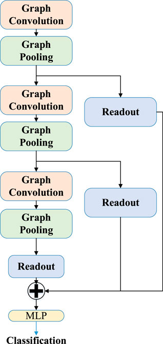
FIGURE 1. Flow chart of neural network classification.

2.2.2 Sliding rules of multilayer supervised networks

In actual crisis supervision and prediction, we must use the dynamic sliding window method to train and test the network many times to ensure the validity of the SAGPOOL method. Specifically, the length of the training set was twice that of the test set and the slide window length. We set the length of the training set to 240-,120- and 60-day windows.

The main process of the dynamic sliding window method is illustrated in the Figure 2. Each paragraph (red vertical line) in Figure 2 represents a single network from the six-layer dynamic networks. For example, the networks in Figure 2 are the second-layer dynamic networks (PCC-PMFG). The tags (equal to 1) of each layer network correspond to the crisis event labels in Table 1 [49–51]. All other tags are equal to 0.

FIGURE 2

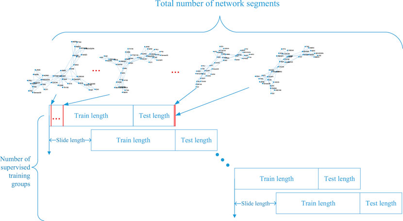
FIGURE 2. (Color online) Window segmentation diagram of the dynamic supervised network.

TABLE 1

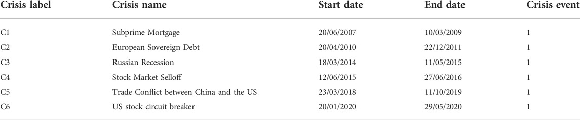
TABLE 1. The table of crisis events.

A general flow chart of MSNA method and the summary of this study are shown in Figure 3.

FIGURE 3

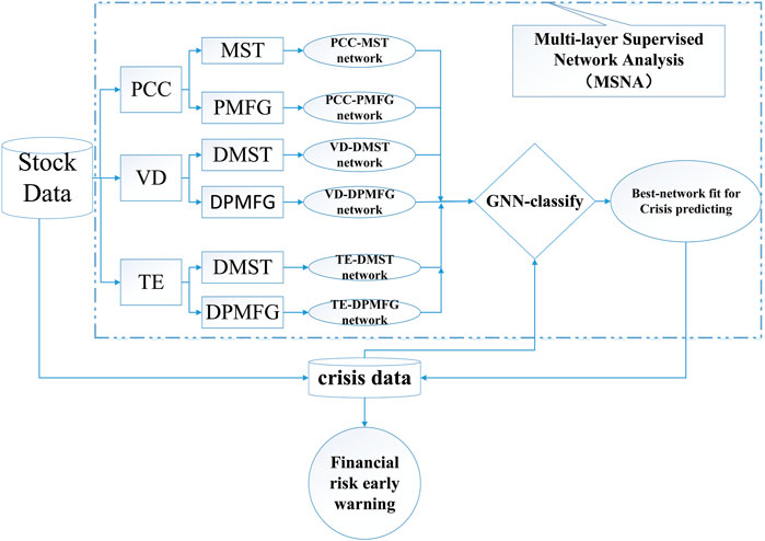
FIGURE 3. (Color online) Flow chart of the multilayer supervised network.

3 Data set

In this study, we chose 37 important stock markets¹ from four continents:Asia (15 stocks), Europe (12 stocks), America (9 stocks) and Oceania (1 stock). The detailed contents of the stocks is listed in Table 2.

TABLE 2

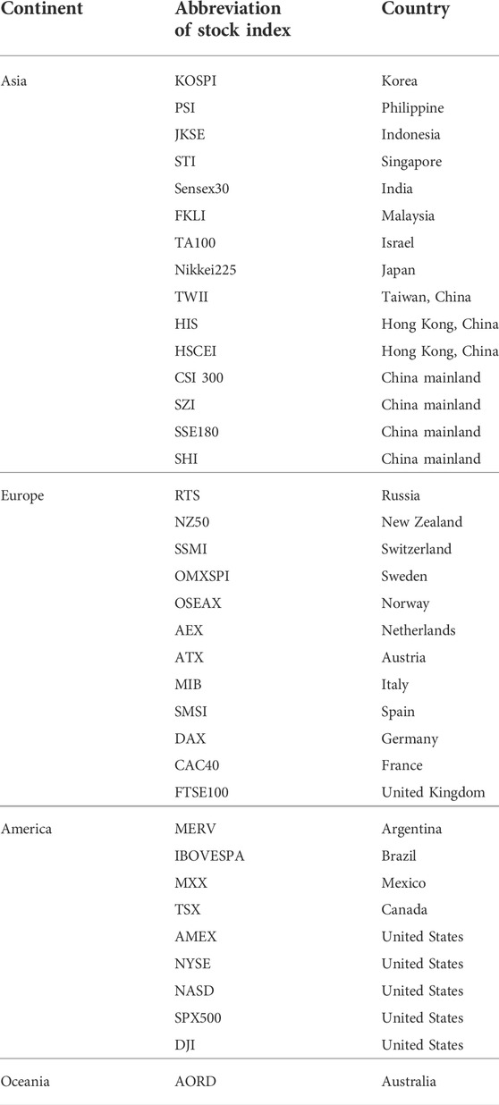
TABLE 2. Stock index list.

Daily indices are considered, while the study period covers approximately 17 years from 1 January 2005, to 3 October 2021. The length of the closing price is 5,124.

4 Result

4.1 Topology parameters and community structures of multilayer networks

Based on multlayer network creation methods, we construct evolving 6-layer networks (PCC-MST,PCC-PMFG,VD-DMST,VD-DPMFG,TE-DMST,TE-DPMFG) on 240-, 120-, and 60-day windows. In this study, we set up Δ = 1, L = 120, M = 37, T = 5,123, Q = 2 and H = 4. The multiplex network of the global financial crisis shown in Figure 3. Figures 4, 5A,B show that DAX (Germany), SPX500 (United States) and STI (Singapore) have the larger degrees in the first layer network. Due to a broader amount of information in the second layer network, DAX (Germany), STI (Singapore), NYSE (United States) and HIS (Hong Kong, China) are all affected. In the third layer network, PSI (Philippine) is the head node of a directed spanning tree network owing to its comparatively earlier opening time, which is similar to Vrost et al [52, 53]. In the fourth-layer network, the NYSE and the SPX500 of the United States are the two most affected stock indices. As can be seen from the DMST in the fifth layer, the in-degree of HSCEI (Hong Kong, China) is zero, which indicates that the HSCEI is the least influenced stock. The most influenced node in the sixth layer network was NASD (United States).

FIGURE 4

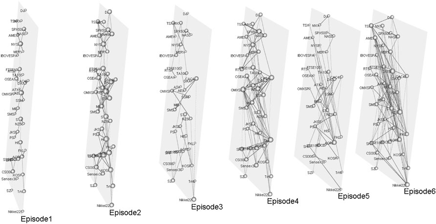
FIGURE 4. (Color online) Multilayer network at the time of global financial crisis.

FIGURE 5

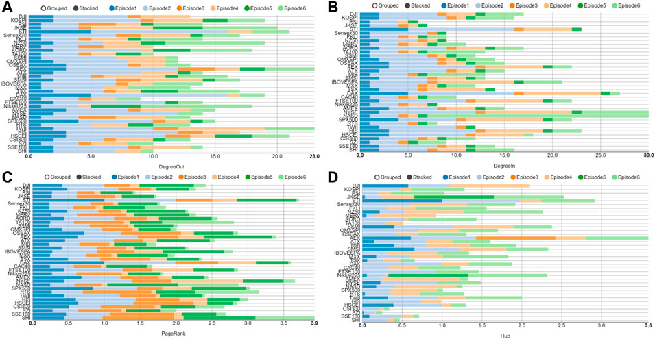
FIGURE 5. (Color online) Parameters of each layer network at the time of global financial crisis.(A) The out-degree of each layer network; (B) The in-degree of each layer network; (C) The PageRank of each layer network; (D) The Hub of each layer network.

As can be seen from the cumulative PageRank values of each layer in Figure 5C, the PageRank values of SHI (China), STI (Singapore), DAX (Germany), and NASD (United States) are higher, which indicates that these stock indexes have strong dissemination power. In Figure 5D, AEX (United States) is at the hub node.

Although the parameters of the individual layer network can provide us with valuable information, the integration of multilayer network information is more important. The parameters of multilayer network at the time of the global financial crisis are shown in Figure 5. As shown in Figure 6A, the AEX (Netherlands), TWII (China), HSCEI (China), Tokyo (Japan) and STI (Singapore) are the most influential stocks. In Figure 6B, NYSE (United States), NASD (United States), STI (Singapore) and HIS (HongKong, China) are the most influenced stocks. From the PageRank index in Figure 6C, NYSE (United States), NASD (United States), SPX500 (United States) DAX (Germany) and SHI (China Mainland) are the most highly transmissible index. In Figure 6D, DAX (United States), AEX (United States), STI (Singapore), FTSE (Britain) are included as the main nodes in Hub index. Figure 6 shows that the results derived from the multilayer network ensemble parameters are more stable than those in the single layer network.

FIGURE 6

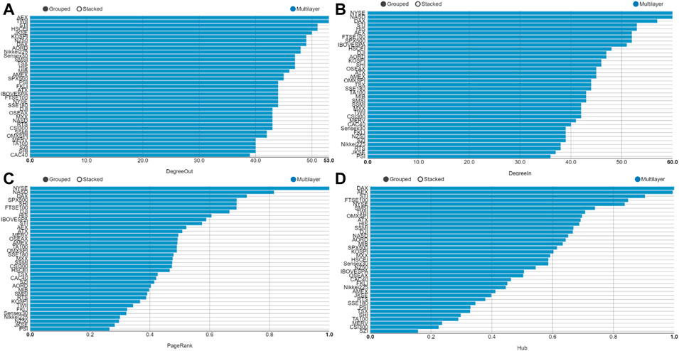
FIGURE 6. (Color online) Parameters of each layer network at the time of global financial crisis. (A) The out-degree of multilayer network, (B) The in-degree of multilayer network, (C) The PageRank of multilayer network, (D) the hub of multilayer network.

To analyze the community relationship of each node in the multilayer network, we use multilayer infomap algorithm [54] to detect the network’s community structure. The results of the community division of the mutilayer network are shown in Figure 7. Figure 6 shows the division of associations in each layer did not differ greatly, especially for layers 1–4. Asian stocks such as FKLI, KOSPI, TA100, Nikkei225, TWII, HIS, HSCEI, CSI300, SZI, SHI, Sensex30, STI belong to one community. The AORD (Australia) and NZ250 (New Zealand) belong to an other society. MXX, DJI, NYSE, NASD and SPX500 are all in one community (American group-1). Ibovessa, Merv, AMEX and TSX belong to a single community (American group-2). OSEAX, OMXSPI, AEX, ATX, MIB, SMSI, DAX, CAC40, FTSE100, SSMI, and RTS are included in one community (the European group). It also underscores that JKSE(Indonesia), of layers 1 and 2, belongs to the European group, while JKSE, of layers 3, 4 and 5 belongs to American group-2.

FIGURE 7

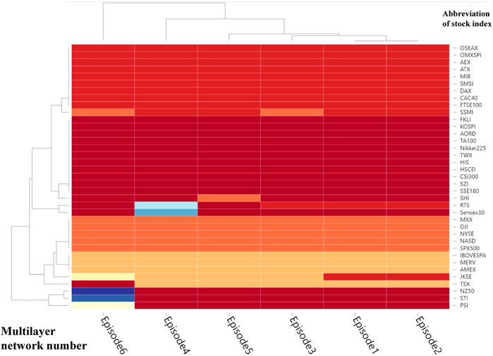
FIGURE 7. (Color online) Community division results of the multilayer network at the beginning of the financial crisis, obtained via a Multi-infomap algorithm. The horizontal axis means the Layer ID, Episode1 to 6 correspond to Layer1 to 6 respectively. The vertical axis shows the abbreviations of all stocks.

In Figure 7, the findings from the distribution of communities indicate that the layer 1(PCC-MST) and layer 2(PCC-PMFG) belong to one community. In addition, the layer 3(VD-DMST) and layer 5 (TE-DMST) are similar to layers 1 and 2. The stock numbers for each community are shown in Figure 8. Communities 1 to 4 correspond to the Asian-Oceania group, European group, American group 1 and American group 2, respectively.

FIGURE 8

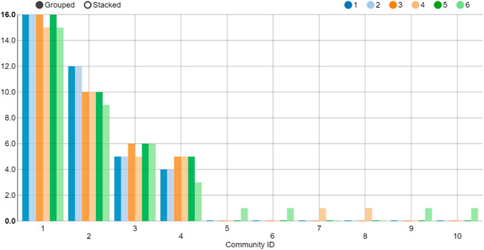
FIGURE 8. (Color online) Quantity statistics in each community at the beginning of the global financial crisis. The horizontal axis indicates the community ID. The vertical axis represents quantities of each Community ID.

We also show the multiplex network and its parameters of the European subprime mortgage crisis in Figures 9, 10, respectively. As shown in Figures 8, 10A, AEX and NYSE are most influenced in the first layer network. AEX, NYSE, HIS and HSCEI of the second-layer network are most influenced. Because of the early opening, PSI is the most influential stock in the third-layer network. OMXSPI (Sweden) is the most influenced stock in the fourth-layer network. In the fifth-layer network, AORD (Australia) is the most influential stock. In the sixth layer network, the most influenced stock was TA100 (Israel).

FIGURE 9

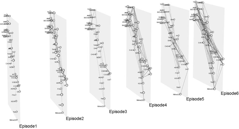
FIGURE 9. (Color online) Multilayer network at the time of European subprime mortgage crisis.

FIGURE 10

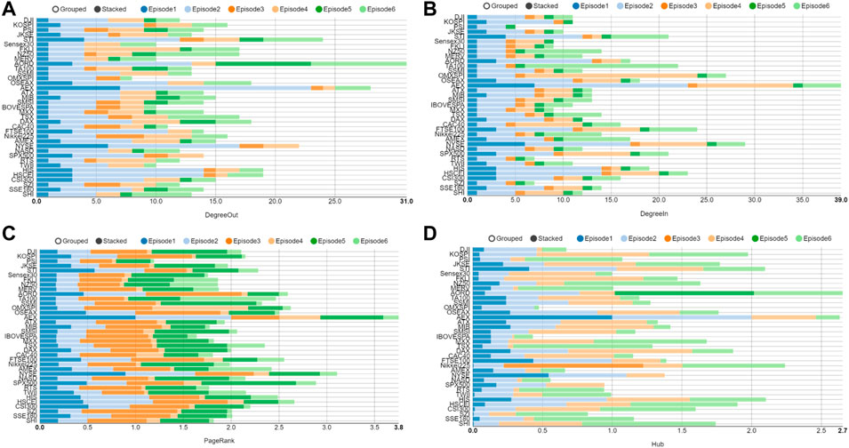
FIGURE 10. Parameters of each layer network at the time of the European subprime mortgage crisis. (A) The out-degree of each layer network; (B) The in-degree of each layer network; (C) The PageRank of each layer network; (D) The Hub each layer network.

In Figure 10C, AEX (Netherlands),NYSE (United States), SPX500 (United States) and HSCEI (China) have a strong infectivity. The hub nodes in Figure 10D are AORD (Australia), AEX (Netherlands), Nikkei225 (Japan) and HIS (China). It can be surmised, by uniting the results of Figures 9, 10 that the European stocks (AEX,OMXSPI) are the most affected and infected during the European subprime mortgage crisis. Due to early opening time of AORD (Australia), PSI (Philippines), and Nikkei225, they have the most influential effect.

The multilayer result during the European subprime mortgage crisis is depicted in Figure 11. The out-/in-degree, PageRank and Hub of AEX (Netherlands) and OMXSPI (Sweden) are all at the forefront. We also present the community division results of the multilayer in Figures 12, 13. The biggest difference between Figures 7, 12 is that MXX, DJI, NYSE, NASD, SPX500, Ibovessa, Merv, AMEX and TSX belong to one community (the American group) durning the European subprime mortgage crisis but belong to two communities (American society-1 and 2) in the Global financial crisis. Further conclusions are illustrated in Figures 8, 13 show that the number of communities in the period of global financial crisis is higher than that in the period of European subprime mortgage crisis period.

FIGURE 11

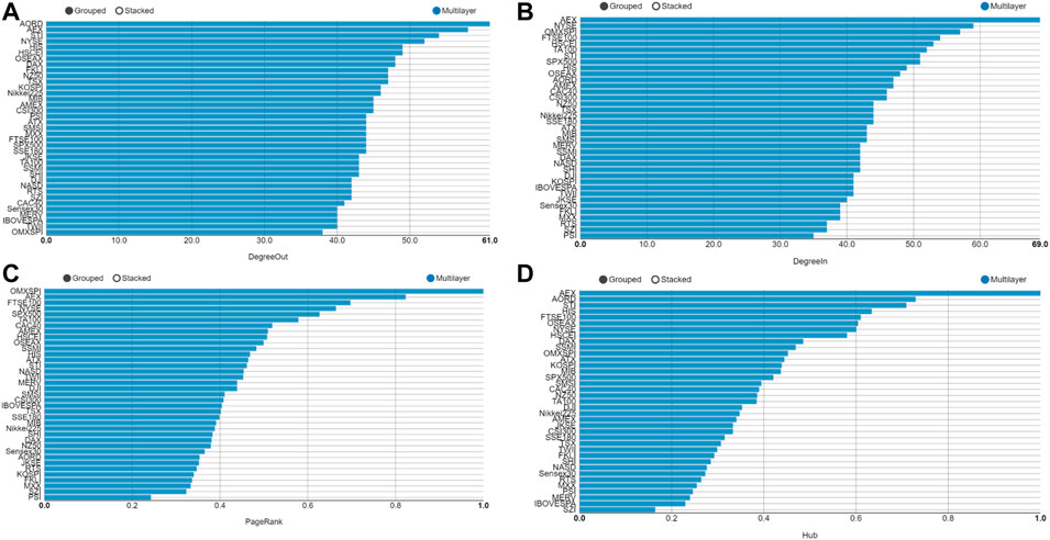
FIGURE 11. Parameters of the multilayer network at the time of European subprime mortgage crisis. (A) The out-degree of the multilayer network; (B) The in-degree of the multilayer network; (C) The PageRank of the multilayer network; (D) The hub of the multilayer network.

FIGURE 12

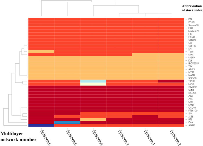
FIGURE 12. Community division results of the multilayer network at the beginning of the European subprime mortgage crisis, obtained by a multi-infomap algorithm.

FIGURE 13

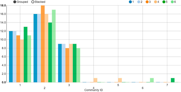
FIGURE 13. Quantity statistics in each community at the beginning of the European subprime mortgage crisis. The horizontal axis means the Community ID. The vertical axis indicates quantities of each Community ID.

4.2 Crisis early warning results based on multilayer supervision networks

Based on the created dynamic multilayer network, we intend to add the crisis events as label values and integrate the supervised characteristics to each dynamic network layer. Because of the weakness of machine learning and neural network in handling feature representation of input dynamic networks, we utilize the GNNC method to fill this technical gap. Specifically, we train and test all six-layer dynamic networks utilizing our MSNA method in 60-day, 120-day and 240-day windows. The detailed results of the three windows are shown in Figure 14 and Table 3. The mean-total-240, mean-total-120, mean-total-60 in Table 3 indicate the mean precision results of MSNA method in 240-,120- and 60-day windows, respectively.

FIGURE 14

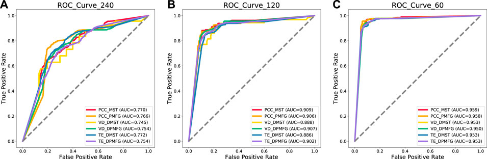
FIGURE 14. Prediction results of all time periods of each window.(A–C) indicate prediction results of all time periods at 240-length scales, 120-length scales and 60-length scales respectively.

TABLE 3

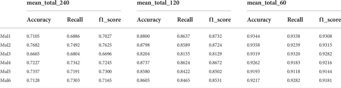
TABLE 3. Mean results of each multilayer networks using MSNA methods.

As shown in Table 3 and Figure 14, the accuracy of financial crisis prediction increases with the reduction of window length. In general, accuracy can properly evaluate the model performance. It represents the prediction correctness of crisis events and non crisis events (all events). Recall indicates the prediction precision of all crisis events. When the model deals with unbalanced sample classification, f1_score can more correctly evaluate the model performance than accuracy and recall. For an ideal early warning model, accuracy, recall and f1_score should be as large as possible. As can be seen from Table 3, when the time window is 60, the lowest f1_score (Mul5) also reaches 0.9144. While the window is 240, the lowest layer (Mul3) is 0.6665. This result confirms the effectiveness of our MSNA method in short sequence crisis prediction. In addition, we also discovered that the fifth-layer (TE-DMST) network has the best performance in a long windows, while the first-layer (PCC-MST) network has the best results in short windows.

Simultaneously, we also intercepted warning results of six periods of financial crisis for statistics. The detailed results of accuracy and ROC curve are displayed in Tables 4–6 and Figures 15–17. Table 6 shows that, in the 240-day window condition, the best performances of the six financial crises prediction are Mul4 (VD-PMFG), Mul2 (PCC-PMFG), Mul4, Mul4, Mul2, and Mul4, respectively. In Table 5 corresponding to 120-length condition, we discover that Mul2 (PCC-DPMFG), Mul1 (PCC-DMST), Mul5 (TE-DMST), Mul1, Mul1, Mul1 have the best performances of 6 financial crises (c1 to c6) prediction, respectively. Table 6 is the result of the accuracy of six financial crisis predictions in a 60-length condition. We can conclude that Mul1, Mul4, Mul1, Mul6, Mul1, and Mul1 have the best performances of the 6 financial crisis (c1 to c6) predictions, respectively. The optimal mean values of the accuracy of the six crises from 240-length to 60-day are Mul2, Mul1, and Mul1, respectively. In summary, the correlation network is the most accurate system for predicting financial crises.

TABLE 4

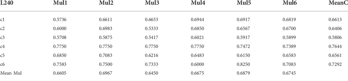
TABLE 4. The mean results of each multilayer network of the six crises in the 240-day window.

TABLE 5

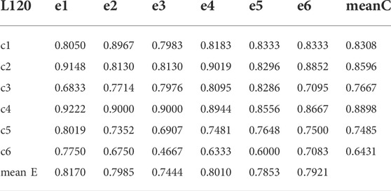
TABLE 5. The mean results of each multilayer network of the six crises in the 120-day window.

TABLE 6

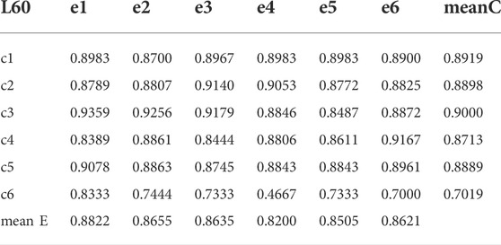
TABLE 6. The mean results of each multilayer network of the six crises in the 60-day window.

FIGURE 15

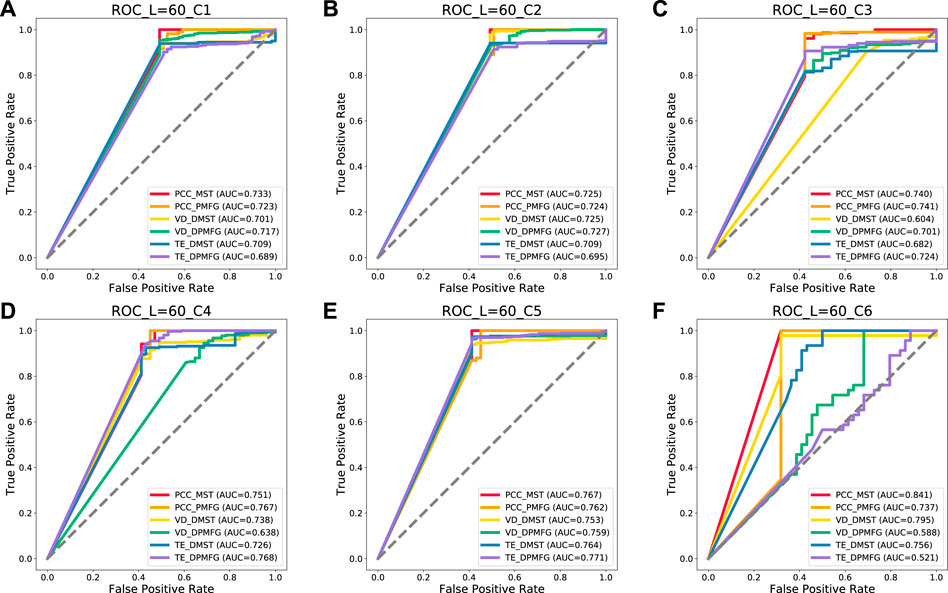
FIGURE 15. Prediction of the six crises of each layer network at 60-day windows. (A–F) indicate the prediction result of each financial crisis. C1 to C6 indicate the following crises: Subprime Mortgage, European Sovereign Debt, Russian Recession, Stock Market Selloff, and Trade Conflict between China and the United States, US stock circuit breaker, respectively.

FIGURE 16

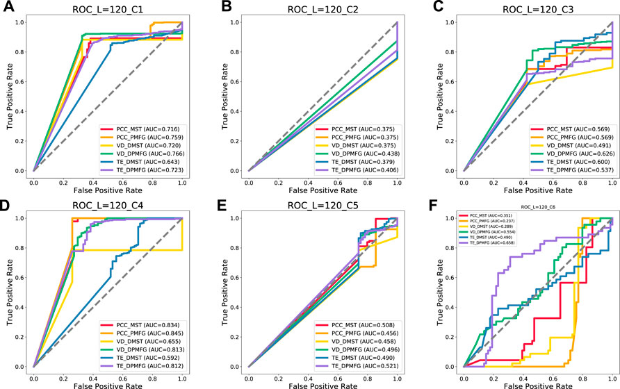
FIGURE 16. Prediction results of each layer of the network at 120-day windows. (A–F) indicate the prediction result of each financial crisis. C1 to C6 indicate the following crises: Subprime Mortgage, European Sovereign Debt, Russian Recession, Stock Market Selloff, and Trade Conflict between China and the United States, US stock circuit breaker, respectively.

FIGURE 17

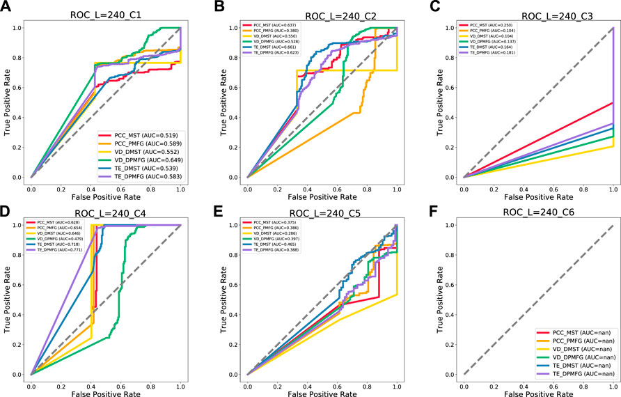
FIGURE 17. Prediction results of each layer of the network at 240-day windows. (A–F) indicate prediction result of each financial crisis. C1–C6 indicate the following crises: Subprime Mortgage Crisis, European Sovereign Debt, Russian Recession, Stock Market Selloff, and Trade Conflict between China and the United States, US stock circuit breaker, respectively.

As can be seen in Figure 15, the PCC-MST, VD-DPMFG, PCC-PMFG, PCC-MST, TE-DPMFG, and PCC-MST networks are the most stable and efficient graphs for predicting the six financial crises of 60-day condition, respectively. In Figures 16, 17, the results of the AUC values in the 120- and the 240-day conditions were not all stable and efficient. In the 120-day condition, there are five efficient networks (VD-DPMFG, VD-DPMFG, PCC-PMFG, PCC-MST, TE-DPMFG) corresponding to c1, c3, c4, c5, and c6, respectively. In the 240-length condition, there are only three efficient networks (VD-DPMFG,PCC-MST,TE-DPMFG) corresponding to c1, c2, and c4, respectively.

5 Conclusion and discussion

Several scholars have proposed various effective methods for financial network construction. For example, Gan et al. applied the threshold method to reduce noise in a pearson correlation network [55]. Further, Marti et al. proposed using the MST method and PCC to construct the network, which resolved the shortcomings of artificial and subjective threshold selection, and likewise simplified the topology of the financial network (M-1) [56]. Because the MST method will result in a loss of important information, Hosseini et al. proposed constructing it using PCC and PMFG (3M-6) [57]. Because there are many nonlinear relationships between financial institutions, analyzing only linear relationships will result in a loss of important information. Therefore, Hosseini et al. applied the TE method to investigate the relationship between several stocks, and utilized DMST to construct the network [58]. Zhang et al. constructed a financial network by employing VD method [59]. Additionally, some scholars have used DCC GARCH t copula [60], GARCH BEKK model [61], symbolic dynamics model [62], and non-linear Granger causality tests [63] to build financial networks.

In this study, we employed PCC, VD, TE, MST, PMFG, DMST, and DPMFG, which are popular among the above methods, to construct a six-layer dynamic financial network. Through the analysis of topological quantities (degree, out-/in-degree, PageRank, Hub, etc.) in multilayer networks, we conclude that in the stage of global financial crisis, the external risk contagion effect and affected intensity of the United States, China, Japan and Singapore were comparatively large. At the stage of the European subprime mortgage crisis, Australia, the Netherlands and Singapore had the greatest external impact, while the Netherlands, the United States, Sweden and the United Kingdom were the most affected. The community division results of the multilayer network show that the community number during the global financial crisis (four communities) was lower than that during the European subprime mortgage crisis (three communities). In short, we use the topological features of the information spillover network between stock indices in various essential places as a training element to improve existing macroeconomic-based warning indicators. The proposed MSNA early warning model, with a multi-layer information spillover network as input variable, has shown excellent early warning effect in empirical studies on real-world datasets and can provide strategic support to regulatory authorities to prevent financial crises.

Further research should be conducted to enhance the accuracy of long-term crisis warning, which is affected by the amount of training data, model overfitting and other factors. For the problem of training set data volume, we will unite the macroeconomic data, sentiment indices and other data in the future, and merge the mixed frequency model [64] to reduce the impact of the data volume of the training set. For model overfitting, we will improve model’s prediction accuracy in the future by adjusting its regularization.

Data availability statement

Publicly available datasets were analyzed in this study. This data can be found here: https://www.wind.com.cn/NewSite/wft.html.

Author contributions

LQ determined the research problems and objectives. LQ and RS analyzed the data and wrote the manuscript. ZW supervised the study and designed project. The authors contributed to manuscript revision and have read approved the submitted version.

Funding

This research was funded by the General project of NSFC: Research on multi-dimensional and multiple contagions of Banking Systemic Financial Risk in structural change (Grant Number. 71973098) and Youth project of NSFC: Financial risk early-warning based on high dimensional supervised network (Grant Number. 12105178).

Conflict of interest

The authors declare that the research was conducted in the absence of any commercial or financial relationships that could be construed as a potential conflict of interest.

Publisher’s note

All claims expressed in this article are solely those of the authors and do not necessarily represent those of their affiliated organizations, or those of the publisher, the editors and the reviewers. Any product that may be evaluated in this article, or claim that may be made by its manufacturer, is not guaranteed or endorsed by the publisher.

Footnotes

¹https://www.wind.com.cn/NewSite/wft.html.

References

1. Frankel JA, Rose AK. Currency crashes in emerging markets: An empirical treatment. J Int Econ (1996) 41(3):351–66. doi:10.1016/S0022-1996(96)01441-9

CrossRef Full Text | Google Scholar

2. Kaminsky G, Lizondo S, Reinhart CM. Leading indicators of currency crises. Staff Pap Int Monet Fund (1998) 45(1):1–48. doi:10.2307/3867328

CrossRef Full Text | Google Scholar

3. Berg A, Pattillo C. Predicting currency crises:. J Int Money Finance (1999) 18(4):561–86. doi:10.1016/S0261-5606(99)00024-8

CrossRef Full Text | Google Scholar

4. Sachs JD, Tornell A, Velasco A, Calvo GA, Cooper RN. Financial crises in emerging markets: The lessons from 1995. Brookings Pap Econ Act (1996) 1996(1):147–215. doi:10.2307/2534648

CrossRef Full Text | Google Scholar

5. Billio M, Casarin R, Costola M, Pasqualini A. An entropy-based early warning indicator for systemic risk. J Int Financial Markets Institutions Money (2016) 45:42–59. doi:10.1016/j.intfin.2016.05.008

CrossRef Full Text | Google Scholar

6. Dastkhan H. Network‐based early warning system to predict financial crisis. Int J Fin Econ (2019) 26(1):594–616. doi:10.1002/ijfe.1806

CrossRef Full Text | Google Scholar

7. Kumar M, Moorthy U, Perraudin W. Predicting emerging market currency crashes. J Empir Finance (2003) 10(4):427–54. doi:10.1016/S0927-5398(02)00068-3

CrossRef Full Text | Google Scholar

8. Klomp J. Causes of banking crises revisited. North Am J Econ Finance (2009) 21(1):72–87. doi:10.1016/j.najef.2009.11.005

CrossRef Full Text | Google Scholar

9. Schularick M, Taylor AM. Credit booms gone bust: Monetary policy, leverage cycles, and financial crises, 1870–2008. Am Econ Rev (2012) 102(2):1029–61. doi:10.1257/aer.102.2.1029

CrossRef Full Text | Google Scholar

10. Greenwood R, Hanson SG, Sheifer A, Sorensen JA. Predictable financial crises[J]. J Financ (2022) 77(2):863–921. doi:10.1111/jofi.13105

CrossRef Full Text | Google Scholar

11. Boonman TM, Jacobs J, Kuper GH, Romero A. Early warning systems for currency crises with real-time data. Open Econ Rev (2019) 30(4):813–35. doi:10.1007/s11079-019-09530-0

CrossRef Full Text | Google Scholar

12. Sornette D, Demos G, Zhang Q, Cauwels P, Zhang Q. Real-time prediction and post-mortem analysis of the Shanghai 2015 stock market bubble and crash. J Invest Strateg (2015) 4:77–95. doi:10.21314/jois.2015.063

CrossRef Full Text | Google Scholar

13. Fricke D. Financial crisis prediction: A model comparison. SSRN J (2017) 3059052:1–9. doi:10.2139/ssrn.3059052

CrossRef Full Text | Google Scholar

14. Tölö E. Predicting systemic financial crises with recurrent neural networks. J Financial Stab (2020) 49:100746–19. doi:10.1016/j.jfs.2020.100746

CrossRef Full Text | Google Scholar

15. Zhu ZY, Liu N. Early warning of financial risk based on K-means clustering algorithm. Complexity (2021) 24:1–12. doi:10.1155/2021/5571683

CrossRef Full Text | Google Scholar

16. Liu LB, Chen C, Wang B. Predicting financial crises with machine learning methods. J Forecast (2022) 41(5):871–910. doi:10.1002/for.2840

CrossRef Full Text | Google Scholar

17. Bouchaud JP. Economics needs a scientific revolution. Nature (2008) 455(7217):1181. doi:10.1038/4551181a

CrossRef Full Text | Google Scholar

18. Farmer JD, Foley D. The economy needs agent-based modelling. Nature (2009) 460(7256):685–6. doi:10.1038/460685a

PubMed Abstract | CrossRef Full Text | Google Scholar

19. Catanzaro M, Buchanan M. Network opportunity. Nat Phys (2013) 9(3):121–3. doi:10.1038/nphys2570

PubMed Abstract | CrossRef Full Text | Google Scholar

20. Battiston S, Farmer JD, Flache A, Garlaschelli D, Haldane AG, Heesterbeek H, et al. Complexity theory and financial regulation: Economic policy needs interdisciplinary network analysis and behavioral modeling[J]. Science (2016) 351(6275):818–9. doi:10.1126/science.aad0299

PubMed Abstract | CrossRef Full Text | Google Scholar

21. Kumar S, Deo N. Correlation and network analysis of global financial indices. Phys Rev E (2012) 86:026101–8. doi:10.1103/PhysRevE.86.026101

PubMed Abstract | CrossRef Full Text | Google Scholar

22. Dima B, Dima SM. Mutual information and persistence in the stochastic volatility of market returns: An emergent market example. Int Rev Econ Finance (2017) 51:36–59. doi:10.1016/j.iref.2017.05.008

CrossRef Full Text | Google Scholar

23. Brunetti C, Harris JH, Mankad S, Michailidis G. Interconnectedness in the interbank market. J Financ Econ (2019) 133(2):520–38. doi:10.1016/j.jfineco.2019.02.006

CrossRef Full Text | Google Scholar

24. Zhang X, Podobnik B, Kenett DY, Stanley HE. Systemic risk and causality dynamics of the world international shipping market. Physica A: Stat Mech its Appl (2014) 415:43–53. doi:10.1016/j.physa.2014.07.068

CrossRef Full Text | Google Scholar

25. Qiu L, Yang H. Transfer entropy calculation for short time sequences with application to stock markets. Physica A: Stat Mech its Appl (2020) 559:125121–0. doi:10.1016/j.physa.2020.125121

CrossRef Full Text | Google Scholar

26. Diebold FX, Yilmaz K. On the network topology of variance decompositions: Measuring the connectedness of financial firms. J Econom (2014) 182(1):119–34. doi:10.1016/j.jeconom.2014.04.012

CrossRef Full Text | Google Scholar

27. Yang Y, Yang H. Complex network-based time series analysis. Physica A: Stat Mech its Appl (2007) 387(5):1381–6. doi:10.1016/j.physa.2007.10.055

CrossRef Full Text | Google Scholar

28. Yang C, Zhu X, Li Q, Chen Y, Deng Q. Research on the evolution of stock correlation based on maximal spanning trees. Physica A: Stat Mech its Appl (2014) 415:1–18. doi:10.1016/j.physa.2014.07.069

CrossRef Full Text | Google Scholar

29. Wang GJ, Xie C, Stanley HE. Correlation structure and evolution of world stock markets: Evidence from pearson and partial correlation-based networks. Comput Econ (2018) 51(3):607–35. doi:10.1007/s10614-016-9627-7

CrossRef Full Text | Google Scholar

30. Tumminello M, Aste T, Matteo TD, Mantegna RN. A tool for filtering information in complex systems. Proc Natl Acad Sci U S A (2005) 102(30):10421–6. doi:10.1073/pnas.0500298102

PubMed Abstract | CrossRef Full Text | Google Scholar

31. Kwon O, Yang JS. Information flow between stock indices. Europhys Lett (2008) 82(6):68003. doi:10.1209/0295-5075/82/68003

CrossRef Full Text | Google Scholar

32. Fiedor P. Networks in financial markets based on the mutual information rate. Phys Rev E (2014) 89(5):052801–7. doi:10.1103/PhysRevE.89.052801

PubMed Abstract | CrossRef Full Text | Google Scholar

33. Park D, Ryu D. Forecasting stock market dynamics using bidirectional long short-term memory. Rom J Econ Forecast (2021) 24:22–34.

Google Scholar

34. McBeth MK, Tokle RJ, Schaefer S. Media narratives versus evidence in economic policy making: The 2008-2009 financial crisis*. Soc Sci Q (2018) 99(2):791–806. doi:10.1111/ssqu.12456

CrossRef Full Text | Google Scholar

35. Samitas A, Kampouris E, Kenourgios D. Machine learning as an early warning system to predict financial crisis. Int Rev Financ Anal (2020) 71:101507. doi:10.1016/j.irfa.2020.101507

CrossRef Full Text | Google Scholar

36. Zhang X, Chen MY, Wang MG, Ge YE, Stanley HE. A novel hybrid approach to Baltic Dry Index forecasting based on a combined dynamic fluctuation network and artificial intelligence method. APPL MATH COMPUT (2019) 361:499–516. doi:10.1016/j.amc.2019.05.043

CrossRef Full Text | Google Scholar

37. Lee J, Lee I, Kang J. Self-attention graph pooling. In: 36th International Conference on Machine Learning; Long Beach, CA (2019). ICML 6661-6670.

Google Scholar

38. Ying R, Morris C, Hamilton WL, You J, Ren X, Leskovec J. Hierarchical graph representation learning with differentiable pooling. Adv Neural Inf Process Syst (2018) 38:4800–10. doi:10.48550/arXiv.1806.08804

CrossRef Full Text | Google Scholar

39. Qiu L, Nan WY. Brain network constancy and participant recognition: An integrated approach to big data and complex network analysis. Front Psychol (2020) 11:1003–24. doi:10.3389/fpsyg.2020.01003

PubMed Abstract | CrossRef Full Text | Google Scholar

40. Gabow HN, Galil Z, Spencer T, Tarjan RE. Efficient algorithms for finding minimum spanning trees in undirected and directed graphs. Combinatorica (1986) 6:109–22. doi:10.1007/BF02579168

CrossRef Full Text | Google Scholar

41. Sandoval L. Structure of a global network of financial companies based on transfer entropy. Entropy (2014) 16(8):4443–82. doi:10.3390/e16084443

CrossRef Full Text | Google Scholar

42. De Domenico M, Solé-Ribalta A, Cozzo E, Kivelä M, Moreno Y, Porter MA, et al. Mathematical formulation of multilayer networks. Phys Rev X (2013) 3(4):041022–15. doi:10.1103/PhysRevX.3.041022

CrossRef Full Text | Google Scholar

43. Bargigli L, di Iasio G, Infante L, Lillo F, Pierobon F. The multiplex structure of interbank networks. Quant Finance (2015) 15(4):673–91. doi:10.1080/14697688.2014.968356

CrossRef Full Text | Google Scholar

44. De Domenico M, Solé-Ribalta A, Omodei E, Gómez S, Arenas A. Ranking in interconnected multilayer networks reveals versatile nodes. Nat Commun (2015) 6:6868–6. doi:10.1038/ncomms7868

PubMed Abstract | CrossRef Full Text | Google Scholar

45. Boccaletti S, Bianconi G, Criado R, Del Genio CI, Gómez-Gardeñes J, Romance M, et al. The structure and dynamics of multilayer networks. Phys Rep (2014) 544(1):121–2. doi:10.1016/j.physrep.2014.07.001

PubMed Abstract | CrossRef Full Text | Google Scholar

46. Cao Y, Liu Z, Li C, Liu Z, Li J, Chua TS. Multi-channel graph neural network for entity alignment[J]. In: ACL 2019-57th Annual Meeting of the Association for Computational Linguistics, Proceedings of the Conference; 2019 Jul 28–Aug 2; Florence, Italy (2020). p. 1452–61. doi:10.18653/v1/p19-1140

CrossRef Full Text | Google Scholar

47. Kipf TN, Welling M. Semi-supervised classification with graph convolutional networks[J]. In 5th International Conference on Learning Representations ICLR 2017 - Conference Track Proceedings; 2017 Apr 24–26; Toulon, France (2017).

Google Scholar

48. Xu K, Li C, Tian Y, Sonobe T, Kawarabayashi KI, Jegelka S. Representation learning on graphs with jumping knowledge networks[J]. In: 35th International Conference on Machine Learning; 2018 Jul 10–15; Stockholm, Sweden (2018). p. 8676–85.

Google Scholar

49. Tommaso B. Systemic risk. GitHub (2022). Available from: https://github.com/TommasoBelluzzo/SystemicRisk/releases/tag/v3.5.0 (Accessed May 18, 2022).

Google Scholar

50. Zhu M, Xu ZX. The impact of the China US trade tensions on China’s stock market. Stud Int Finance (2021) 4:3–12. doi:10.16475/j.cnki.1006-1029.2021.04.001-en

CrossRef Full Text | Google Scholar

51. Cortes F, Lindner P, Malik S, Segoviano Basurto M. A comprehensive multi-sector tool for analysis of systemic risk and interconnectedness (SyRIN). IMF Work Pap (2018) 18(14):1–54. doi:10.5089/9781484338605.001

CrossRef Full Text | Google Scholar

52. Baumöhl E, Kočenda E, Lyócsa Š, Výrost T. Networks of volatility spillovers among stock markets. Physica A: Stat Mech its Appl (2018) 490(C):1555–74. doi:10.1016/j.physa.2017.08.123

CrossRef Full Text | Google Scholar

53. Výrost T, Lyócsa Š, Baumöhl E. Granger causality stock market networks: Temporal proximity and preferential attachment. Physica A: Stat Mech its Appl (2015) 427:262–76. doi:10.1016/j.physa.2015.02.017

CrossRef Full Text | Google Scholar

54. De Domenico M, Lancichinetti A, Arenas A, Rosvall M. Identifying modular flows on multilayer networks reveals highly overlapping organization in interconnected systems. Phys Rev X (2015) 5(1):011027–11. doi:10.1103/PhysRevX.5.011027

CrossRef Full Text | Google Scholar

55. Mizutaka S, Tanizawa T. Robustness analysis of bimodal networks in the whole range of degree correlation. Phys Rev E (2016) 94(2-1):022308–7. doi:10.1103/PhysRevE.94.022308

PubMed Abstract | CrossRef Full Text | Google Scholar

56. Gan SL, Djauhari MA. New York stock exchange performance: Evidence from the forest of multidimensional minimum spanning trees. J Stat Mech (2015) 2015(12):P12005–23. doi:10.1088/1742-5468/2015/12/P12005

CrossRef Full Text | Google Scholar

57. Nie CX, Song FT. Constructing financial network based onPMFGand threshold method. Physica A: Stat Mech its Appl (2018) 495:104–13. doi:10.1016/j.physa.2017.12.037

CrossRef Full Text | Google Scholar

58. Hosseini SS, Wormald N, Tian TH. A weight-based information filtration algorithm for stock-correlation networks. Physica A: Stat Mech its Appl (2021) 563:125489–14. doi:10.1016/j.physa.2020.125489

CrossRef Full Text | Google Scholar

59. Zhang DY, Broadstock DC. Global financial crisis and rising connectedness in the international commodity markets. Int Rev Financ Anal (2020) 68:101239–11. doi:10.1016/j.irfa.2018.08.003

CrossRef Full Text | Google Scholar

60. Müller FM, Righi MB. Numerical comparison of multivariate models to forecasting risk measures. Risk Manag (2018) 20(1):29–50. doi:10.1057/s41283-017-0026-8

CrossRef Full Text | Google Scholar

61. Liu XY, An HZ, Li HJ, Chen ZH, Feng SD, Wen SB. Features of spillover networks in international financial markets: Evidence from the G20 countries. Physica A: Stat Mech its Appl (2017) 479:265–78. doi:10.1016/j.physa.2017.03.016

CrossRef Full Text | Google Scholar

62. Stavroglou SK, Pantelous AA, Stanley HE, Zuev KM. Hidden interactions in financial markets. Proc Natl Acad Sci U S A (2019) 116(22):10646–51. doi:10.1073/pnas.1819449116

PubMed Abstract | CrossRef Full Text | Google Scholar

63. Kim JM, Lee N, Hwang SY. A copula nonlinear granger causality. Econ Model (2020) 88:420–30. doi:10.1016/j.econmod.2019.09.052

CrossRef Full Text | Google Scholar

64. Xu QF, Zhuo X, Jiang CX, Sun F, Huang X. Reverse restricted MIDAS model with application to US interest rate forecasts. Commun Stat - Simulation Comput (2021) 50(2):462–82. doi:10.1080/03610918.2018.1563148

CrossRef Full Text | Google Scholar