Quantum K-nearest neighbors classification algorithm based on Mahalanobis distance

Mahalanobis distance is a distance measure that takes into account the relationship between features. In this paper, we proposed a quantum KNN classification algorithm based on the Mahalanobis distance, which combines the classical KNN algorithm with quantum computing to solve supervised classification problem in machine learning. Firstly, a quantum sub-algorithm for searching the minimum of disordered data set is utilized to find out K nearest neighbors of the testing sample. Finally, its category can be obtained by counting the categories of K nearest neighbors. Moreover, it is shown that the proposed quantum algorithm has the effect of squared acceleration compared with the classical counterpart.

1 Introduction

With the development of era, the amount of global data is increasing exponentially every year. People often use machine learning to extract valid information from large amounts of data. However, with the increase of the amount of data, classical machine learning algorithms need a lot of time. How to design an efficient learning algorithm has become a major difficulty in the field of machine learning. At this point, the speed advantage of quantum computing over classical computing in solving certain specific problems has led more and more scholars to think about how to use quantum computing to solve the problem more efficiently and has given rise to a new field of research – quantum machine learning (QML). Quantum machine learning uses quantum superposition, quantum entanglement and other basic principles of quantum mechanics to realize computing tasks [1]. That is to say, QML is a quantum version of machine learning algorithms, which can achieve an exponential or squared quantum acceleration effect.

In recent years, researchers have studied quantum machine learning algorithms in depth and have achieved outstanding works in many branches of research, such as quantum K-nearest neighbor (QKNN) algorithm [2–4], quantum support vector machine (QSVM) [5, 6], quantum neural network (QNN) [7–9] and so on [10, 11]. These algorithms take full advantage of quantum superposition and entanglement properties, allowing them to achieve quantum acceleration compared to classical algorithms.

QKNN algorithms is a combination of quantum computing and classical algorithm. In 2013, Lloyd proposed a distance-based supervised learning quantum algorithm [12], which has exponential acceleration effect compared with classical algorithms. In 2014, Wiebe raised a QKNN algorithm based on inner product distance [2] with squared acceleration effect. In 2017, Ruan realized a QKNN algorithm based on Hamming distance [3], which has a time complexity of $O\left({\left({\mathit{log}}_{2}M\right)}^3\right)$ in the case of an optimal threshold. These algorithms measure the similarity between samples according to different distance metrics and achieve quantum acceleration. However, none of these distance measures consider the connection between individual attributes in the samples, which leads to many limitations in practical applications.

In this paper, we propose an efficient quantum version of KNN algorithm based on Mahalanobis distance. The algorithm architecture is similar to the classical algorithm. Similarly, we also notice two key points in designing the KNN algorithm. One is to efficiently compute the distance between M training samples and test sample, and the other is to find the smallest K number of samples. However, compared with the existing algorithms, the proposed algorithm takes fully account of the sample correlations and uses Mahalanobis distance to eliminate the interference of correlations between variables. Finally, the test samples are successfully classified using the algorithm of searching for K-nearest neighbor samples and the calculated Mahalanobis distance. The algorithm achieves a quadratic speedup in terms of time complexity.

2 Preliminaries

In this section, we briefly review the main process of the classical KNN classification and the Mahalanobis distance.

2.1 K-nearest neighbors classification algorithm

KNN algorithm is a common supervised classification algorithm, which works as follows: given a test sample and a training sample set, where the training sample set contains M training samples. Then, we compute the distances between the test sample and the M training samples, and find the K nearest training samples by comparing these distances. If the majority of the K nearest neighbor training samples of the test sample belong to a class, then the class of the test sample is that class [13, 14]. In the KNN algorithm, the most complex step is to compute the distance between the test sample and all training samples. Moreover, the computational complexity increases with the number and dimensionality of the training samples. In order to classify the test samples with dimension N and perform the distance metric with M N-dimensional training samples, we need to perform $O\left(MN\right)$ operations.

The general process of classical KNN classification can be summarized in the following points.

1) Choose an appropriate distance metric and calculate the distance between the test sample with M training samples.

2) Find the K training samples with closest distance to the test sample.

3) Count the class with the highest frequency among these K training samples, and that class is the class of the sample to be classified.

Although the K-nearest neighbor algorithm has better performance and accuracy, we should note that the choice of the distance metric is extremely important [15]. In general, we use the Euclidean distance as the metric. In fact, the Euclidean distance is just an integration of the two samples’ deviations on each variable by treating all variables equally, which has some limitations in terms of data relevance. Instead, we use a generalization of the Euclidean distance: the Mahalanobis distance, which calculates the distance between two points by covariance and is an effective method to calculate the similarity of two unknown samples. Unlike the Euclidean distance, it takes into account the correlation between various variables. The difference between Euclidean distance and Mahalanobis distance is shown in Figure 1.

FIGURE 1

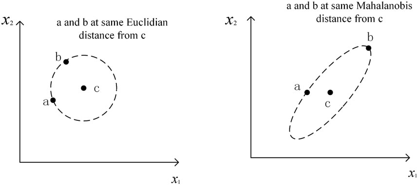
FIGURE 1. The difference between Euclidean distance and Mahalanobis distance.

As shown above, we can easily find that the Mahalanobis distance is better than the Euclidean distance. The Mahalanobis distance can be used to reasonably unify the data between different features, since its computation takes into account the fact that the scale units are different in different directions.

2.2 The Mahalanobis distance

Mahalanobis distance is an effective metric to calculate the distance between two samples, which considers the different feature attributes. It also has two advantages as follows. 1) It is independent of the magnitude and the distance between two points is independent of the measurement units of the original data. 2) The Mahalanobis distance can also eliminate the interference of correlation between variables.

In this paper, the training samples and the test sample are combined into a data set $\left\{x_1,x_2{,x}_3,\cdots x_M,v\right\}$, which can be described as a column vector composed of N characteristic attributes ${\left\{z_1,z_2,z_3\cdots z_N\right\}}^T$ μ_i is the expected value of i th element, ${\mu }_i=E\left(z_i\right)$. The correlation between the dimensions of these samples is expressed by the covariance matrix Σ, i.e.,

$\mathrm{\Sigma }=\left[\begin{array}{cc}\hfill \begin{array}{c}\hfill E\left[\left(z_1-{\mu }_1\right)\left(z_1-{\mu }_1\right)\right]\hfill \\ \hfill E\left[\left(z_2-{\mu }_2\right)\left(z_1-{\mu }_1\right)\right]\hfill \end{array}\hfill & \hfill \begin{array}{cc}\hfill \cdots \hfill & \hfill E\left[\left(z_1-{\mu }_1\right)\left(z_N-{\mu }_N\right)\right]\hfill \\ \hfill \cdots \hfill & \hfill E\left[\left(z_2-{\mu }_2\right)\left(z_N-{\mu }_N\right)\right]\hfill \end{array}\hfill \\ \hfill \begin{array}{c}\hfill ⋮\hfill \\ \hfill E\left[\left(z_N-{\mu }_N\right)\left(z_1-{\mu }_1\right)\right]\hfill \end{array}\hfill & \hfill \begin{array}{cc}\hfill \ddots \hfill & \hfill ⋮\hfill \\ \hfill \cdots \hfill & \hfill E\left[\left(z_N-{\mu }_N\right)\left(z_N-{\mu }_N\right)\right]\hfill \end{array}\hfill \end{array}\right](1)$

where, the ij term in the covariance matrix (the ij term is a covariance) is

${\mathrm{\Sigma }}_{ij}=cov\left(z_i,z_j\right)=E\left[\left(z_i-{\mu }_i\right)\left(z_j-{\mu }_j\right)\right].(2)$

The Mahalanobis distance between data points x and y is

$D=\sqrt{{\left(x-y\right)}^T{\mathrm{\Sigma }}^{-1}\left(x-y\right)},(3)$

where Σ is the covariance matrix of x and y. By multiplying the inverse of the covariance matrix based on Euclidean distance, the effect of correlation between the data can be eliminated.

As description above all, it is not difficult to find approaches to calculate the Mahalanobis distances between M training samples and the test sample

$\sum _{i=1}^M{d}_i=\sum _{i=1}^M\sqrt{\left(x_i-v\right){\mathrm{\Sigma }}^{-1}\left(x_i-v\right)}.(4)$

Σ represents the covariance matrix of X and v. The covariance matrix is a semi-positive definite symmetric matrix that allows for eigenvalue decomposition. $\mathrm{\Sigma }={\sum }_{j=1}^N{\lambda }_j\left|{\mu }_j\right.⟩⟨{\mu }_j|$, where λ_j is the eigenvalue, and μ_j is the corresponding feature vectors. Then, Eq. 4 can be redescribed as

$\sum _{i=1}^M{d}_i=\sum _{i=1}^M\sqrt{⟨x_i-v|\sum _{j=1}^N{{\lambda }_j}^{-1}\left|{\mu }_j\right.⟩⟨{\mu }_j|\left|x_i-v\right.⟩}.(5)$

While we need to get the K minimum distance of them, thus we just need to get

$\sum _{i=1}^M{d}_i=\sum _{i=1}^M\sum _{j=1}^N{\lambda }_j^{-1}⟨{\mu }_j|x_i-v.⟩(6)$

3 The proposed quantum K-nearest neighbor classification algorithm

In this section, we mainly describe the significant steps of the proposed quantum KNN classification algorithm.

3.1 Calculating the Mahalanobis distance

Computing similarity is an important subprogram in classification algorithms. For the classification of non-numerical data, Mahalanobis distance is one of the popular ways to calculate similarity. Here, we describe a quantum method to calculate Mahalanobis distance between x_i and v in parallel.

A1: Prepare the superposition state

According to Eq. 6, we need to prepare the required quantum states $\frac{1}{\sqrt{M}}{\sum }_{i=1}^M|i⟩|x_i-v⟩$ and the covariance matrix Σ. For simple description, x_i − v is preprocessed on the basis of classical data to make it normalized data.

Here, we firstly introduce the preparation process of $\frac{1}{\sqrt{M}}{\sum }_{i=1}^M\left|i\right.⟩\left|x_i-v\right.⟩$. The process can be briefly divided into two steps. First, prepare the superposition type $\frac{1}{\sqrt{M}}{\sum }_{i=1}^M\left|i\right.⟩$, and then the data x_i − v is accessed through quantum random access memory [16]. Next, we will explain these two steps in detail.

At first, we prepare $m={\mathit{log}}_2\left(M+1\right)$ quantum qubit in the state of $\left|000\cdots 000\right.⟩$(${\left|0\right.⟩}^{\otimes m}$), and then a Hadamard gate operation is performed once for each qubit to get the state:

$H^{\otimes m}\left|000\cdots 000\right.⟩=\frac{1}{\sqrt{2^m}}\sum _{i=0}^{2^m-1}\left|i\right.⟩(7)$

However, our aim is to get the initial superposition qubits $\left|\alpha \right.⟩=\frac{1}{\sqrt{M}}{\sum }_{i=1}^M\left|i\right.⟩$. Since M may not be a power of 2, the state is obtained with the help of a quantum comparator [17], as show in Figure 2.

FIGURE 2

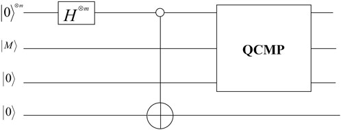
FIGURE 2. Prepare the quantum state $\left|\alpha \right.⟩$.

With the help of two auxiliary particles $\left|0\right.⟩\left|0\right.⟩$, we can judge the value space of index i through the quantum comparator. The details are shown as follows:

$U_1\left({\left|0\right.⟩}^{\otimes m}\left|0\right.⟩\left|0\right.⟩\right)\to \frac{1}{\sqrt{2^m}}\sum _{i=0}\left|i\right.⟩\left|0\right.⟩\left|1\right.⟩+\frac{1}{\sqrt{2^m}}\sum _{0<i\le M}\left|i\right.⟩\left|0\right.⟩\left|0\right.⟩+\frac{1}{\sqrt{2^m}}\sum _{i>M}\left|i\right.⟩\left|1\right.⟩\left|0\right.⟩(8)$

Then we measure the auxiliary particles to obtain the target state. When the result is $\left|0\right.⟩\left|0\right.⟩$ and the probability of measuring success is $\frac{M}{2^m}$, the require quantum state $\left|\alpha \right.⟩=\frac{1}{\sqrt{M}}{\sum }_{i=1}^M\left|i\right.⟩$ will be obtained after $O\left(\frac{M}{2^m}\right)=O\left(1\right)$ times.

Finally, we access the classical data based on the quantum random access memory theory. It is assumed that there exists a quantum channel that can access the data stored in quantum random access memory, and the data x_i − v is stored in the form of classical data in M storage units in QRAM. So, we can access x_i − v efficiently through a black box O_x in $O\left({\mathit{log}}_{2}MN\right)$. The specific operation is as follows:

$\frac{{\sum }_{i=1}^M\left|i\right.⟩\left|0\right.⟩}{\sqrt{M}}\stackrel{O_x}{\to }\frac{{\sum }_{i=1}^M\left|i\right.⟩\left|x_i-v\right.⟩}{\sqrt{M}}(9)$

Next, we show how to get the covariance matrix. Since the covariance matrix Σ is semi-positive definite, we can implement it by Hamiltonian simulation [18]. Assuming that $\mathrm{\Sigma }={\sum }_{j=1}^N{\lambda }_j\left|{\mu }_j\right.⟩⟨{\mu }_j|$ [19]. Prepare a quantum black box given access to Hermitian matrix Σ, any time t, and errors ϵ, operate with approximate unitary precision ϵ through a quantum circuit U₂. Then the state e^iΣt can be obtained.

$‖U_2-e^{i\mathrm{\Sigma }t}‖\le ϵ(10)$

Compared with the classical algorithm, the state e^iΣt obtained by the quantum circuit has exponential acceleration effect. Its time complexity is $O\left(polylogN\right)$.

A2: Compute distances

In the following, we talk about how to compute the Mahalanobis distances between the test sample and the training samples, i.e., Eq. 6. Obviously, by performing the steps of A1, we have obtained the state $\frac{{\sum }_{i=1}^M\left|i\right.⟩\left|x_i-v\right.⟩}{\sqrt{M}}$. To obtain the form of Eq. 6, we need to perform the phase estimation and controlled rotation. Specifically, it can be divided into two sub-processes.

Step 2.1 Adding one register in the state |0⟩ to get the state $\frac{{\sum }_{i=1}^M\left|i\right.⟩|0\rangle \left|x_i-v\right.⟩}{\sqrt{M}}$. Then, we perform an unitary operation on the second and the third registers controlled by U₂ to achieve the phase estimation. At this point, we obtain the quantum state $\left|{\mathrm{\Psi }}_1\right.⟩$,

$\left|{\mathrm{\Psi }}_1\right.⟩=\frac{\sum _{i=1}^M\left[\sum _{j=1}^N⟨u_j|x_i-v⟩|i\rangle \left|\frac{\stackrel{\sim }{{\lambda }_j}{t}_0}{2\pi }\right.⟩\left|u_j\right.⟩\right]}{\sqrt{M}}.(11)$

In phase estimation, $\frac{\widetilde{{\lambda }_j}{t}_0}{2\pi }\in \left[\mathrm{0,1}\right)$, which is a period that numerical values outside the range are projected into the range. So that we should limit the scope of $\frac{{\lambda }_j{t}_0}{2\pi }$ belong to $\left[-\frac{1}{2},\frac{1}{2}\right)$. To ensure the accuracy of results, some algorithmic assumptions are made here, assuming that $\left|{\lambda }_j\right|\in \left[\frac{1}{k},1\right]$. Due to λ_j ≥ 0, t₀ > 0 (t₀ is the minimum time for simulating the covariance matrix e^iΣt), when t₀ ≤ π, it can ensure $\frac{{\lambda }_j{t}_0}{2\pi }\in \left[-\frac{1}{2},\frac{1}{2}\right)$. Usually, we take t₀ = π to make the results obtained from the phase estimation more accurate.

Step 2.2 Adding an auxiliary qubit $\left|0\right.⟩$, and performing a controlled rotation operation $\left(CR\right)$ on the second register of $\left|{\mathrm{\Psi }}_1\right.⟩$, which can effectively extract the information in the quantum register to the amplitude of the quantum state. The process is as follows.

Suppose that θ ∈ R, $\tilde{\theta }$ is a d-bit finite precision representation of θ. The controlled rotation U_θ can make:

$\begin{array}{c}\hfill |\tilde{\theta }\rangle |0\rangle \to |\tilde{\theta }\rangle \left(f\left(\tilde{\theta }\right)\left|0\right.⟩+\sqrt{1-{f\left(\tilde{\theta }\right)}^2}\left|1\right.⟩\right).\end{array}(12)$

So, the following operation can be achieved by setting the relevant parameters.

$\begin{array}{c}\hfill \left|\frac{\widetilde{{\lambda }_j}{t}_0}{2\pi }\rangle \right|0\rangle \to |\frac{\widetilde{{\lambda }_j}{t}_0}{2\pi }\rangle \left(f\left(\frac{\widetilde{{\lambda }_j}{t}_0}{2\pi }\right)|0\rangle +\sqrt{1-{f\left(\frac{\widetilde{{\lambda }_j}{t}_0}{2\pi }\right)}^2}|1\rangle \right).\end{array}(13)$

Apparently, if $f\left(x\right)=\frac{2\pi }{t_0}x$, we can obtain $\left|{\mathrm{\Psi }}_2\right.⟩$.

$\begin{array}{c}\hfill \left|{\mathrm{\Psi }}_2\right.⟩=\frac{\sum _{i=1}^M\left|i\right.⟩\sum _{j=1}^N⟨u_j|x_i-v⟩|\frac{\stackrel{\sim }{{\lambda }_j}{t}_0}{2\pi }\rangle |u_j\rangle \left(\frac{c}{\stackrel{\sim }{{\lambda }_j}}\left|0\right.⟩+\sqrt{1-{\left(\frac{c}{\stackrel{\sim }{{\lambda }_j}}\right)}^2}\left|1\right.⟩\right)}{\sqrt{M}}\end{array}(14)$

From the preceding information, we know that the Mahalanobis distance is $d_i={\sum }_{j=1}^N{\lambda }_j^{-1}⟨{\mu }_j|x_i-v⟩$, so $\left|{\mathrm{\Psi }}_2\right.⟩$ can be rewrite to

$\begin{array}{cc}\hfill \left|{\mathrm{\Psi }}_2\right.⟩& =\frac{\sum _{i=1}^M\left|i\right.⟩d_i|\frac{\stackrel{\sim }{{\lambda }_j}{t}_0}{2\pi }\rangle \left|u_j\right.⟩\left|0\right.⟩}{\sqrt{M}}+\frac{\sum _{i=1}^M\left|i\right.⟩\sum _{j=1}^N\sqrt{1-{\left(\frac{c}{\stackrel{\sim }{{\lambda }_j}}\right)}^2}⟨u_j|x_i-v⟩|\frac{\stackrel{\sim }{{\lambda }_j}{t}_0}{2\pi }\rangle \left|u_j\right.⟩\left|1\right.⟩}{\sqrt{M}}\hfill \end{array}(15)$

For applying the Mahalanobis distance calculated by the above process to the classification algorithm, we have to use the amplitude estimation (AE) algorithm to transfer the distance information to qubits [20]. Then, we get the state about distance information $\left|{\mathrm{\Psi }}_3\right.⟩=\frac{{\sum }_{i=1}^M\left|i\right.⟩\left|d_i\right.⟩}{\sqrt{M}}$. This process uses R iterations of Grover operators and the error is less than δ, where R and δ satisfy $R\ge \frac{\pi (\pi +1)}{\delta }$.

3.2 Searching K minimum distances

In this section, we use the state $\left|{\mathrm{\Psi }}_3\right.⟩$ acquired by previous chapter to search the K minimum distances through quantum minimum search algorithm [21, 22].

Step 1. The set $D=\left\{D_1,D_2\cdots D_K\right\}$ represents K training sample closest to test sample $v=\left\{v_1,v_2,v_3\cdots v_N\right\}$ in the training sample. The initialization D is a random selection of K samples from the training samples.

Step 2. By Grover’s algorithm, we get one point x_i at a time from the quantum state $\left|{\mathrm{\Psi }}_3\right.⟩$. If that point is closer to the test sample than some points in D_k, i.e., $d\left(v,x_i\right)<d\left(v,D_k\right)\left(k\in \left[1,K\right]\right)$, the ith point is used to replace the point D_k in D, and k is the $\mathit{max}\left\{d\left(v,D_k\right)\right\}\left(k\in \left[1,K\right]\right)$.

Step 3. In order to get the k points with the smallest distance, repeat Step 2 to make q smaller and smaller (q is the number of remaining points in the set Q) until q = 0. That is, we find the k points that are closest to the test sample.

To analyze the time complexity of the above process more easily, we introduce a set Q, which is a subset of X beyond of D and smaller than some points in set D from the test sample. q is the number of points in set Q. In the following, we will use the size of q to analyze the performance of the algorithm after each operation. Repeating Step 2 k times can decrease q to $\frac{3}{4}q$. When q > 2K, it can be reduced to $\frac{1}{2}q$ by calling Oracle operation $O\left(\sqrt{\frac{KM}{q}}\right)$ times. When q is decreased to q ≤ 2K, the calling time of Oracle is $K\sqrt{\frac{M}{K}+\frac{M}{2K}+\frac{M}{4K}+\cdots }$. Then, if q is decreased to 0, the total time is $O\sqrt{KM}$. At this time, the points in set D are the K training samples closest to the test sample.

4 Complexity analysis

Let us start with discussing the time complexity of the whole algorithm. As mentioned above, the algorithm contains three steps:

A1. Preparation of the initial state.

A2. Parallel computation of the martingale distance.

A3. Search for K nearest neighbor samples.

An overview of the time complexity of each step is shown in Table 1. A detailed analysis of each step of this algorithm is depicted as follows.

TABLE 1

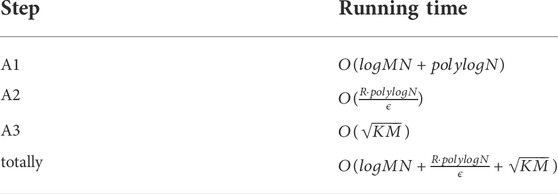
TABLE 1. The time complexity of the algorithm.

In step A1, $\frac{1}{\sqrt{M}}{\sum }_{i=1}^M\left|i\right.⟩\left|x_i-v\right.⟩$ can be generated in time O(logMN) with the help of quantum comparator and QRAM. Then, the Hamiltonian simulation has been performed to make the covariance matrix Σ. So, the time complexity of A1 is $O\left(logMN+polylogN\right)$. In part of A2, we utilize phase estimation and controlled rotation to compute the distance, and then translate the information into quantum state. According to Ref. [1], the time complexity of phase estimation is $O\left(\frac{T_u}{ϵ}\right)$, where T_u is the time of preparing the unitary operator e^iΣt and $\frac{1}{ϵ}=2^{-m}$ e^iΣt is obtained by Hamiltonian simulation, therefore, the time complexity is $O\left(polylogN\right)$. In a word, the time complexity is $O\left(\frac{polylogN}{ϵ}\right)$. Afterwards, in order to transfer the distance information to qubits, we have to perform the AE algorithm R times (discussed in step A2.2). Hence, the total time complexity of the quantum algorithm for computing the Mahalanobis distance is $O\left(logMN+\frac{R\cdot polylogN}{ϵ}\right)$. In Step A3, the time complexity of searching is analyzed in Section 3.2, that is $O(\sqrt{KM})$.

Therefore, the time complexity of the whole algorithm is $O\left(logMN+\frac{R\cdot polylogN}{ϵ}+\sqrt{KM}\right)$. Compared with the classical KNN classification algorithm with $O\left(MN\right)$ time complexity, it has quadratic acceleration.

5 Conclusion

In this paper, we combine the ideology of quantum computation with classical KNN classification algorithm to propose a quantum KNN classification algorithm based on Mahalanobis distance. First, we quantified the similarity measure algorithm based on the Mahalanobis distance. Then, K nearest neighbor samples are filtered using the quantum minimum search algorithm. Compared with other quantum KNN classification algorithms based on Hamming distance or Euclidean distance, the Mahalanobis distance used in this paper overcomes the drawback that individual feature attributes with different degrees of variation play the same role in calculating the distance metric and excludes the interference of different degrees of correlation between variables. When the training sample is very large, the time complexity of the algorithm is $O\left[logMN+\frac{R\cdot polylogN}{ϵ}+\sqrt{KM}\right]$, which has a quadratic acceleration effect. In conclusion, we give a complete quantum classification algorithm. By executing the proposed algorithm, the classification classes of the test samples can be obtained. Moreover, our work gives the sub-algorithm to calculate the Mahalanobis distance, which can be directly applied to the designing of other quantum machine learning algorithms, such as clustering.

Data availability statement

The raw data supporting the conclusions of this article will be made available by the authors, without undue reservation.

Author contributions

All authors listed have made a substantial, direct, and intellectual contribution to the work and approved it for publication.

Funding

This work was supported by the National Natural Science Foundation of China (Grants Nos. 61,772,134, 61,976,053 and 62,171,131), the Higher Educational Key Laboratory for Flexible Manufacturing Equipment Integration of Fujian Province (Xiamen Institute of Technology), the research innovation team of Embedded Artificial Intelligence Computing and Application at Xiamen Institute of Technology (KYTD202003), and the research innovation team of Intelligent Image Processing and Application at Xiamen Institute of Technology (KYTD202101).

Conflict of interest

The authors declare that the research was conducted in the absence of any commercial or financial relationships that could be construed as a potential conflict of interest.

Publisher’s note

All claims expressed in this article are solely those of the authors and do not necessarily represent those of their affiliated organizations, or those of the publisher, the editors and the reviewers. Any product that may be evaluated in this article, or claim that may be made by its manufacturer, is not guaranteed or endorsed by the publisher.

References

1. Nielsen MA, Chuang IL. Quantum computation and quantum information. Math Structures Comput Sci (2002) 17(6):1115.

Google Scholar

2. Nathan W, Kapoor A, Svore K. Quantum algorithms for nearest-neighbor methods for supervised and unsupervised learning. Quan Inf Comput (2014) 15(3):316–56. doi:10.26421/qic15.3-4-7

CrossRef Full Text | Google Scholar

3. Yue R, Xue X, Liu H, Tan J, Li X. Quantum algorithm for k-nearest neighbors classification based on the metric of hamming distance. Int J Theor Phys (Dordr) (2017) 56(11):3496–507. doi:10.1007/s10773-017-3514-4

CrossRef Full Text | Google Scholar

4. Hai VT, Chuong PH, Bao PT. New approach of knn algorithm in quantum computing based on new design of quantum circuits. Informatica (2022) 46(5):2022. doi:10.31449/inf.v46i5.3608

CrossRef Full Text | Google Scholar

5. Rebentrost P, Mohseni M, Lloyd S. Quantum support vector machine for big data classification. Phys Rev Lett (2014) 113(13):130503. doi:10.1103/physrevlett.113.130503

PubMed Abstract | CrossRef Full Text | Google Scholar

6. Zhang R, Wang J, Jiang N, Hong L, Wang Z. Quantum support vector machine based on regularized Newton method. Neural Networks (2022) 151:376–84. doi:10.1016/j.neunet.2022.03.043

PubMed Abstract | CrossRef Full Text | Google Scholar

7. Farhi E, Neven H. Classification with quantum neural networks on near term processors (2018). arXiv preprint arXiv:1802.06002.

Google Scholar

8. Nathan K, Bromley TR, Arrazola JM, Schuld M, Quesada N, Lloyd S. Continuous-variable quantum neural networks. Phys Rev Res (2019) 1:033063. doi:10.1103/physrevresearch.1.033063

CrossRef Full Text | Google Scholar

9. Cong I, Choi S, Lukin MD. Quantum convolutional neural networks. Nat Phys (2019) 15(12):1273–8. doi:10.1038/s41567-019-0648-8

CrossRef Full Text | Google Scholar

10. Wu C, Huang F, Dai J, Zhou N. Quantum susan edge detection based on double chains quantum genetic algorithm. Physica A: Stat Mech its Appl (2022) 605:128017. doi:10.1016/j.physa.2022.128017

CrossRef Full Text | Google Scholar

11. Zhou N, Xia S, Ma Y, Zhang Y. Quantum particle swarm optimization algorithm with the truncated mean stabilization strategy. Quan Inf Process (2022) 21(2):42–23. doi:10.1007/s11128-021-03380-x

CrossRef Full Text | Google Scholar

12. Lloyd S, Mohseni M, Rebentrost P. Quantum algorithms for supervised and unsupervised machine learning (2013). arXiv preprint arXiv:1307.0411.

Google Scholar

13. Dang Y, Jiang N, Hu H, Ji Z, Zhang W. Image classification based on quantum k-nearest-neighbor algorithm. Quan Inf Process (2018) 17(9):239–18. doi:10.1007/s11128-018-2004-9

CrossRef Full Text | Google Scholar

14. Zhou N, Liu X, Chen Y, Du N. Quantum k-nearest-neighbor image classification algorithm based on k-l transform. Int J Theor Phys (Dordr) (2021) 60(3):1209–24. doi:10.1007/s10773-021-04747-7

CrossRef Full Text | Google Scholar

15. Yu K, Guo G, Jing L, Lin S. Quantum algorithms for similarity measurement based on Euclidean distance. Int J Theor Phys (Dordr) (2020) 59(10):3134–44. doi:10.1007/s10773-020-04567-1

CrossRef Full Text | Google Scholar

16. Giovannetti V, Lloyd S, Maccone L. Quantum random access memory. Phys Rev Lett (2008) 100(16):160501. doi:10.1103/physrevlett.100.160501

PubMed Abstract | CrossRef Full Text | Google Scholar

17. Wang D, Liu Z, Zhu W, Li S. Design of quantum comparator based on extended general toffoli gates with multiple targets. Comput Sci (2012) 39(9):302–6.

Google Scholar

18. Rebentrost P, Steffens A, Marvian I, Lloyd S. Quantum singular-value decomposition of nonsparse low-rank matrices. Phys Rev A (Coll Park) (2018) 97(1):012327. doi:10.1103/physreva.97.012327

CrossRef Full Text | Google Scholar

19. He X, Sun L, Lyu C, Wang X. Quantum locally linear embedding for nonlinear dimensionality reduction. Quan Inf Process (2020) 19(9):309–21. doi:10.1007/s11128-020-02818-y

CrossRef Full Text | Google Scholar

20. Brassard G, Høyer P, Mosca M, Tapp A. Quantum amplitude amplification and estimation (2000). arXiv preprint arXiv:quant-ph/0005055.

Google Scholar

21. Gavinsky D, Ito T. A quantum query algorithm for the graph collision problem (2012). arXiv preprint arXiv:1204.1527.

Google Scholar

22. Durr C, Høyer P. A quantum algorithm for finding the minimum (1996). arXiv preprint quant-ph/9607014.

Google Scholar