Metamaterial characterization from far-field acoustic wave measurements using convolutional neural network

Identifying the material properties of unknown media is an important scientific/engineering challenge in areas as varied as in-vivo tissue health diagnostics and metamaterial characterization. Currently, techniques exist to retrieve the material parameters of large unknown media from elastic wave scattering in free-space using analytical or numerical methods. However, applying these methods to small samples on the order of few wavelengths in diameter is challenging, as the fields scattered by these samples become significantly contaminated by diffraction from the sample edges. Here, we propose a method to extract the material parameters of small samples using convolutional neural networks trained to learn the mapping between far-field echoes and the material parameters. Networks were trained with synthetic time domain echo data obtained by simulating the free-space scattering of sound from unknown media underwater. Results show that neural networks can accurately predict effective material parameters such as mass density, bulk modulus, and shear modulus even when small training sets are used. Furthermore, we demonstrate in experiments executed in a water tank that the networks trained with synthetic data can accurately estimate the material properties of fabricated metamaterial samples from single-point echo measurements performed in the far-field. This work highlights the effectiveness of our approach to identify unknown media using far-field acoustic reflection dominated by diffraction fields and will open a new avenue toward acoustic sensing techniques.

Introduction

Extracting material parameters of unknown objects using far-field scattered elastic waves is an essential challenge for applications such as acoustic imaging, non-destructive evaluation, and metamaterial characterization. Conventional approaches typically apply numerical or computational methods to invert the wave equation and obtain the properties of the medium under investigation. In these approaches the medium is probed in free-space with acoustic waves and the scattered sound is processed to extract all of the components of material parameter tensors such as mass density and stiffness. However, these methods are limited to large-sized samples where diffraction from the sample edges does not disturb too much the scattered fields [1, 2]. Also, these methods typically require probing the sample from multiple directions to obtain all the desired properties.

However, in many cases including metamaterial design and in-vivo tissue diagnostics, the unknown objects are elastically small having diameters of a few wavelengths of the probing wave and the influence of diffraction is significant. This makes the aforementioned approaches ineffective and unable to produce all the elastic properties of interest. For instance, ultrasound elastography and impediography are used to extract only a small number of stiffness tensor components and impedance of abnormal tissues. Changes in these material properties could sometimes be linked to pathological tissue changes [3, 4], which suggests that tissue diagnostics could improve significantly if all the mechanical properties of these complex, anisotropic media were measured (instead of just a few) including all the stiffness and mass density tensor components.

Techniques reduce the influence of diffraction in small-sized samples have been studied, but most solutions are incompatible with free-space diagnostics methods. For example, waveguides are extensively used to remove the effect of edge diffraction [5–14]. However, these methods are not applicable when the objects cannot be placed in waveguides (e.g., non-destructive evaluation such as tissue diagnostics) or when the existence of waveguides can adversely affect the measurement itself [15] (e.g., metamaterial characterization underwater).

A recent study has shown that, instead of mitigating the effects of diffraction, complex spatial diffraction patterns obtained in near-field measurements can be used to effectively extract the material parameters of small metamaterial samples with the help of machine learning algorithms [16]. However, near-field measurements are not always available, e.g., in-vivo tissue diagnostics. Nevertheless, it has also been shown that echolocating animals use far-field scattered wave to discriminate acoustically small objects such as fish [17], which suggests that the information contained in the diffracted fields could be extracted from far-field single point measurements.

Here, we propose a method to estimate the material parameters from single point far-field scattered wave (echo) measurements. In our approach, we utilize convolutional neural networks (CNNs) to map the complex patterns induced by edge diffraction in the time domain echoes to material parameters such as mass density, bulk modulus, and shear modulus. Moreover, we show that this method requires probing the unknown material from only one direction, in contrast to conventional analytical methods that require many directions of incidence [1, 2]. Results show that CNNs trained with synthetic time domain echoes can effectively predict these material parameters. Importantly, we show that our CNN trained with synthetic data can process actual measurements produced by a hydrophone and can accurately predict the material parameters of fabricated metamaterial samples, which demonstrates that our method is robust to measurement errors.

Methods

Experimental setup

Figure 1A illustrates the experimental setup used to evaluate the material parameters of a sample under test from far-field scattered fields. In the setup, a small sample with known geometry and unknown material parameters is placed underwater and ensonified by a point source. The far-field backscattered acoustic wave (echo) is recorded by a receiver co-located with the source. The diffraction from the small sample edges generates patterns in the far-field echoes which are determined by the mechanical properties of the sample. Without loss of generality, in this paper the sample is isotropic and thus its elastic behavior is determined by mass density (ρ), bulk modulus (K), and shear modulus (G). We also assume the lossless sample is non-resonant and thus its dispersion is negligible.

FIGURE 1

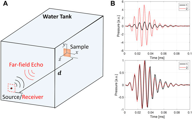
FIGURE 1. Schematic of material characterization using far-field acoustic echoes. (A) A small sample of known geometry and unknown material parameters is ensonified by a point source and echoes are measured by a receiver co-located with the source. (B) Far-field echoes from two different materials show complex time domain variation. The top and bottom panels show echoes before and after normalization. The change in material parameters result in echo amplitude and shape variations.

We consider a rectangular sample of width W, height H, and thickness T in a background medium of known material parameters (ρ₀, K₀, G₀). The sample is ensonified by a point source situated a distance d in front of the sample. The distance d is chosen large enough to assure that the evanescent field components scattered by the sample attenuate enough at the receiver.

Figure 1B shows examples of far-field echoes determined by two material parameter sets [(ρ = 400 kg/m³, K = 0.5 GPa, G = 30 kPa) and (ρ = 6,000 kg/m³, K = 12 GPa, G = 50 GPa)] for a scenario in which the source produces a 7-cycle Gaussian pulse of full width at half maximum (FWHM) bandwidth 20% centered at 120 kHz in a water background (ρ₀ = 1,000 kg/m³, K₀ = 2.25 GPa, G = 0 Pa) and W = H = 4λ, T = 0.16λ, d = 15λ. Here λ = 12 mm is the wavelength corresponding to 120 kHz. The material dispersion is considered small enough so that ρ, K, and G are approximately constant in the frequency band excited. The echoes were simulated using a three-dimensional time-domain solver of the elastic wave equation included in the k-Wave toolbox [18]. Figure 1B depicts two types of echo differences. The first is an amplitude variation (top) mostly caused by different mechanical impedances and the second corresponds to relative phase variations between the various frequencies contained in the acoustic pressure, which translate in slight echo pattern changes in certain regions of the signal (bottom). The latter are caused by how the fields scattered by the sample edges (i.e., diffracted fields) interfere in the far-field. Our method seeks to map these pattern changes to the material parameters that produced them.

Material parameter retrieval using CNNs

Convolutional neural networks are known for their excellent performance in pattern recognition tasks. For instance, they are used with great success for image recognition and classification [19, 20]. Recent studies in acoustics also showed that CNNs work well with acoustic data to identify and classify sounds in both time- (1D) and time-frequency domains (2D). In these works, the marine mammal species were classified using the sounds produced by animals using CNNs [21, 22]. Our goal here is to solve a related regression problem by training CNNs directly on the time-domain echo data to learn the edge-diffraction induced patterns of temporal echoes (see Figure 1B) and map them to the material parameter tuple (ρ, K, G).

Mathematically, the trained CNNs should provide the closed-form mapping $g:\mathcal{F}\to \mathcal{M}$, where $\mathcal{F}$ is the set that contains far-field echoes and $\mathcal{M}$ is the N-dimensional set of unknown material parameters. Finding g is a complicated problem. However, finding the inverse mapping $g^{-1}:\mathcal{M}\to \mathcal{F}$ is a much easier task. For instance, with given material parameter tuple $m\in \mathcal{M}$, the corresponding far-field echo $f\in \mathcal{F}$ can be simulated or even measured experimentally. Here, to estimate g, we compute numerically $f\in {\mathcal{F}}_T$ for a range of material parameters $m\in {\mathcal{M}}_T$ and train a CNN using this data. The symbols ${\mathcal{F}}_T$ and ${\mathcal{M}}_T$ stand for the two subsets used for training the CNN. The trained CNN extrapolates g for data in the entire $\mathcal{M}$. To assess the prediction performance, the trained CNNs are tested on a separate dataset (test set) $f\in {\mathcal{F}}_V=g^{-1}({\mathcal{M}}_V)$, where the ground truth values of material parameters $m\in {\mathcal{M}}_V$ are known and ${\mathcal{M}}_V\cap {\mathcal{M}}_T=\varnothing$ is the empty set. Equally important, we will see that the trained CNN also provides insight into the salient echo features that identifies the sample.

The set of material parameters $\mathcal{M}$ for which g is defined is chosen depending on application. For example, if we want to determine the effective macroscopic properties of a metamaterial sample, we choose $\mathcal{M}$ to encompass all the possible material parameters the sample could have. To illustrate the method in an example, we consider a metamaterial sample designed to operate underwater and whose elastodynamic behavior and effective material parameters were determined in our previous work [16] (see Figure 2). These effective properties obtained with a different method will be used to validate the approach described here. The metamaterial has W = H = 50 mm, T = 2 mm, and consists of copper spheres with a diameter of 2 mm pressure fitted inside a 3D-printed polylactic acid (PLA) matrix. The fabricated metamaterial sample has the same geometry and size as used in the simulations of far-field echoes. Far-field echoes reflected by this metamaterial will be measured to characterize the material properties of the sample using our proposed approach.

FIGURE 2

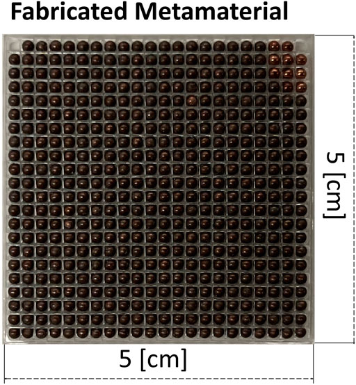
FIGURE 2. Fabricated metamaterial sample consisting of copper spheres embedded in a PLA matrix.

In this design, a single unit cell consists of a copper sphere inside an empty square of PLA and everything is permeated by water. The material parameters of copper are ρ = 8,960 kg/m³, K = 123 GPa, and G = 45 GPa and the surrounding water has the properties listed above. Hence, the fabricated artificial material is expected to have effective macroscopic properties between those of water and copper. However, the exact values depend strongly on several unknown factors such as the friction force between the PLA and the spheres and the exact material properties of the plastic. Similar to [16], we choose the size of $\mathcal{M}$ conservatively to cover the material parameters of our fabricated sample, namely, ρ ∈ (400, 6,000) kg/m³, K ∈ (0.5, 12) GPa, and G ∈ (0, 50) GPa.

The source position and properties are the same as used in the example shown in Figure 1. Namely, the source is placed directly in front of the sample at d = 185 mm away from it. The source ensonifies the metamaterial with a 7-cycle Gaussian pulse centered at 120 kHz. Synthetic echoes were generated by randomly sampling the material parameters $m=(\rho ,K,G)\in {\mathcal{M}}_T\subset \mathcal{M}$. The mass density was sampled following a uniform distribution. The elastic moduli K and G cover large intervals of several orders of magnitudes and thus their logarithms were sampled uniformly. For each m we simulated the far-field echoes f = g⁻¹(m). The echoes were simulated using k-Wave at a sampling rate of 1 MHz. Each echo consists of 314 samples (which corresponds to 0.314 ms long signals) and is long enough to contain the diffraction patterns. A total of 2000 echoes were generated and divided into training and test sets with a ratio of 4:1. In this work, we followed the paradigm described in [23] where test sets are used to assess the loss function during training to prevent overfitting and to assess the final performance of the network.

In the following, we will show that the prediction from trained CNNs on synthetic test sets show good estimation of the material parameters, and the accuracy improves when trained with a second training dataset of narrower range informed by the first set. More importantly, we will show that the CNNs estimate very well the material parameters of the fabricated metamaterial sample and provide very close values to those reported in [16].

Results

Material parameter estimation in a large material space

The CNN used in this work consists of three convolutional layers followed by two fully-connected layers. The inputs are 1D signals of 314 samples that represent time domain echoes. The first convolutional layer has 16 channels and a kernel size of 1 × 5 samples and is followed by a 1 × 2 max-pooling layer. The second and third convolutional layers have 32 and respectively 64 channels with kernel sizes of 1 × 10 and respectively 1 × 15 samples. Both of these convolutional layers are also followed by 1 × 2 max-pooling layers. All three convolutional layers use rectified linear units (ReLUs) activation functions. The two fully-connected layers consist of 2048 nodes and employ ReLU activation functions. The output layer consists of three nodes that represent the estimated material parameters. The three output nodes were linearly mapped to values between 0 and 1, and thus all outputs are equally weighted to compute the mean-square-error (MSE) loss. The converged loss curves shown in Supplementary Figure S1 of the supplementary material illustrate that the networks were trained without overfitting the training datasets.

Figures 3A–C show the estimated material parameters for the media represented in the test set. Given the wide range of elastic moduli covering multiple orders of magnitude, K and G (Figures 3A,B) are plotted on logarithmic scales and the mass density (Figure 3C) is plotted on a linear scale. The scattered plots with circular dots indicate the estimation versus ground truth value and the red solid lines show the ground truth vs. ground truth lines that become the indicator of correct prediction. The mean and confidence interval of the predicted material parameters calculated from 12–13 uniformly divided ranges of the material parameters are depicted with blue lines and error bars, respectively. The confidence interval was determined as ± 2σ of the mean, where σ is the standard deviation in each range. If the estimated material parameters followed normal distributions, this would indicate 95% confidence intervals. Although the distributions of our output variables are unknown, we verified that 93% of the data fall within the ± 2σ confidence intervals.

FIGURE 3

FIGURE 3. Test set estimation of bulk modulus (A,D), shear modulus (B,E), and mass density (C,F). Bulk and shear moduli are plotted on log scales. Dotted arrows indicate predicted values using the measured echo from the metamaterial sample, and the highlighted regions illustrate the confidence intervals for those predictions. The first row shows estimated values in the large $\mathcal{M}$ space and the second row shows those from the reduced material space ${\mathcal{M}}^{\prime }$. The confidence intervals (error bars) are significantly smaller for the lower row. The estimated values from the metamaterial sample bounded by the confidence interval highlighted in (D–F) show excellent agreement with the reported values published in [16].

Figures 3A–C show that the estimated material parameters match well the real values. One exception is the shear modulus for which smaller values have negligible influence on the scattered acoustic field. Consequently, low G media behave elastically like acoustic fluids and the exact shear modulus value is irrelevant from the point of view of elastic waves scattering, consistent with previous findings [16, 24].

After assessing the CNN performance using the test set analysis, we analyze the neural network ability to process experimental measurements inevitably affected by experimental errors. The experiment was performed in a cube-shaped water tank with a side length of 50 cm (Figure 4A). A single Teledyne-Reson TC 4013 hydrophone was placed in front of the sample a distance d = 185 mm away from it to accurately replicate the setup shown in Figure 1. The hydrophone plays the role of source and receiver. The source pulse used in the experiment was identical to the one used for synthesizing the training and test datasets, i.e., a 7-cycle Gaussian broadband pulse centered at 120 kHz. The incident pulse was measured 3 cm in front of the sample to measure the incident field amplitude and thus calibrate the amplitude of the backscattered field. Before submerging the sample into the water tank and doing the measurement, the sample was degassed in a vacuum chamber to remove any possible air bubble formation at the surface and inside the matrix, which influences the sample reflectivity.

FIGURE 4

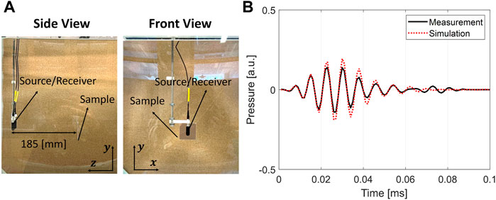
FIGURE 4. Measurement setup (A) and simulated echo using the predicted material parameters (B). The far-field echo simulated using the predicted material parameters shows excellent match with the measurement, and demonstrates that the CNN estimates well the effective material parameters of the sample.

The measured echo shown in Figure 4 (solid line) is passed through the CNN. The estimated material parameters are $\bar{\rho }=1833.2$ kg/m³, $\bar{K}=2.63$ GPa, and $\bar{G}=256$ MPa and the confidence intervals of the estimation were ρ ∈ (782–3,632)kg/m³, K ∈ (1.82–4.57) GPa, and G ∈ (39.8 MPa −4.79 GPa). The estimated effective material parameters were roughly in the same range as the previously reported values [16]. To increase the precision of the estimation we train a second CNN in a smaller material parameter space ${\mathcal{M}}^{\prime }$ obtained using the ± 2σ confidence intervals given above. As a result, the volume of ${\mathcal{M}}^{\prime }$ reduces by a factor of 15 compared to the original space $\mathcal{M}$.

Material parameter estimation in the reduced material space

The training approach described in the previous section was repeated with the smaller material parameter space ${\mathcal{M}}^{\prime }$. Given the smaller ${\mathcal{M}}^{\prime }$, a total of 850 simulations were generated and divided into training and test sets with a ratio of 4:1. Figures 3D–F show the estimations for the test set. The second CNN was able to estimate the material parameters significantly better than the first CNN, as reflected in a smaller confidence intervals than these shown in Figures 3A–C. The second CNN performs better than the first CNN because its output cover a much smaller space than the first CNN. Consequently, the training set of the second CNN samples more densely the network’s output space leading to a better interpolation of the outputs than the first CNN.

After verifying that the CNN performs well, we passed the measured echo through the CNN to obtain the effective material parameters of the fabricated sample. The estimated effective material parameters are highlighted together with their confidence intervals in Figures 3D–F. The estimated values are $\bar{\rho }=1251.3$ kg/m³, $\bar{K}=2.45$ GPa, and $\bar{G}=74.1$ MPa and match very well previously reported values for the same metamaterial sample [16]. For reference, the effective material parameters reported in the past work were $\bar{\rho }=1285.1$ kg/m³, $\bar{K}=2.5$ GPa, and $\bar{G}=0.72$ MPa. The two sets of values are within 2.6% and 2% of each other for the mass density and the bulk modulus, respectively. The discrepancy in the predicted shear moduli is irrelevant, given that low values of G have no influence on the scattering characteristics of the metamaterials, as explained earlier. To further test the robustness of the trained CNN, we have used an echo produced by the same metamaterial sample but for a different position of the source/receiver. In this additional experiment, the metamaterial sample was moved by 2 mm from its original position. (see Supplementary Figure S2).

To further validate the CNN estimations, we performed another numerical simulation with the estimated material parameters and compared the numerically simulated echo against the measurement. The measured and simulated echoes show an excellent match. The small differences are unavoidable experimental errors caused, for example, by the scattering from the physical hydrophone, which contaminates the measured echo in the 0.7–0.8 ms interval. However, we will show in the following that the disturbances due to these errors have little influence on the parameter estimation.

Analysis of echo features targeted by the CNN

Neural networks are excellent at mapping patterns in complicated input signals to output quantities that influence these patterns. An interesting opportunity arises in which we can probe the CNN to understand salient features in the input echoes that facilitate this mapping. Specifically, we performed an analysis in which the input echoes were occluded with a sliding window of size five samples, which is equivalent to the kernel size of the first convolutional layer. We zeroed the echo inside the occluded window and passed the modified signal to the network. The variation of the CNN outputs provides significant information about echo regions targeted by the CNN.

We applied this method in two scenarios. First, we occluded the measured echo which we tested our CNN upon (Figure 4B). Second, the occlusion analysis was applied to all the echoes in the test set for the second CNN trained to process the reduced material space ${\mathcal{M}}^{\prime }$.

Figure 5A presents again the measured echo and Figures 5B–D show the material parameters predicted with the occluded echo. The horizontal axis in Figures 5B–D is the starting point of the occlusion window. For instance, t = 0 ms in Figure 5B indicates the occlusion window was placed from t = 0 ms–0.005 ms. The regions that were most sensitive to the estimation of material parameters are highlighted in each figure. The results show that the sensitive regions for predicting the bulk modulus and the mass density were around t = 0.02 ms and t = 0.04 ms, which correspond to the early and tail regions of the echo pulse (see Figure 5D). On the other hand, it can be seen that the region targeted by the CNN to estimate the shear modulus was between 0.03 and 0.045 ms, which corresponds to the mid-to-tail part of the echo. It is also interesting to note that the disturbance caused by experimental errors at t = 0.07–0.08 ms has caused a variation in the shear modulus which translated in a larger than expected estimated value of 74.1 MPa. But this error has not influenced the other two material parameters, which further demonstrates that the influence of the shear modulus is represented in the latter part of the echo signal.

FIGURE 5

FIGURE 5. Measured echo (A) and the average of the normalized echoes in the test set (E). Prediction change in bulk modulus (B,F), shear modulus (C,G), and mass density (D,H) when input echoes were occluded with sliding time window. The top row illustrates the output material parameters by occluding the measured echo, where the case of no occlusion is plotted with red dotted line. The bottom row illustrates normalized variation of the output parameters where the dotted lines illustrate the mean from the test set and the shaded regions illustrate ± one standard deviation regions. Regions that are most sensitive to changes are highlighted with a vertical band.

To generalize this observation, we performed the same analysis to the simulated echoes in the test set. Figure 5E shows the averaged waveform (solid line) of the normalized 170 echoes in the test dataset, and the ± one standard deviation region (shaded areas). Together these provide an idea of the echo waveforms produced by various material parameters. Figures 5F–H show the average variation in each material parameter and up to one standard deviation away from the average (shaded region) as a result of the occlusion. The quantities are normalized to the case when no occlusion was applied. These metrics represent the relative sensitivity to the occlusion. The targeted regions for the bulk modulus and mass density were consistent with the analysis applied only to the measured echo.

Between the two sensitive regions, t = 0.04 ms was more sensitive ($\sim 2$ folds) to the change in material parameters, indicating that the CNN may be more relying on this region. This is understandable because the initial part of the echo represents the specular reflection, and thus has the same shape independent on the material parameters. However, this region still plays a significant role in the CNN decisions most likely because the early echo peaks represent time references used to measure the timing of subsequent peaks.

Interestingly, Figure 5G shows that the CNN is targeting different regions for G than the other two parameters, most notably the later parts of the echo consistent with Figure 5C. Figure 5C shows an additional echo region of interest than 5 g because the simulated test echoes obtained for relatively small values of G are essentially zero in the region 0.07–0.08 ms (see Figure 5A). As a result, occluding this region influenced by the experimental errors has no effect on the CNN output.

Discussion

In this work, we proposed a convolutional neural network-based method for characterizing material properties of unknown small material samples in free-space from single point far-field measurements. The success of our method relies on two factors, namely the excellent ability of CNNs to deal with pattern recognition tasks and a judicious generation of training datasets. Unlike conventional methods that attempt to mitigate the diffraction from the sample using large samples and multiple directions of incidence, our approach maps the unique diffraction patterns occurring in the time-domain echoes to the material parameters that produced these patterns. Moreover, analysis of the CNNs provide important insights into what parts of the echoes are targeted by the networks.

This work presents a multi-tier method in which the accuracy of the CNN increases with each level. Each level produces closed-form expressions of the material parameters versus time-domain echo for increasingly smaller material parameter space that converges towards the effective material properties. The advantage of this method is the significant reduction in the training set size at the expense of training more networks.

The CNNs were trained with synthetic data obtained in unsupervised numerical simulations, so that the training procedure is fast and inexpensive. This is in contrast with other machine learning approaches that rely on slow and expensive measurements for training. Remarkably, our CNNs trained with numerical simulations maintain ability to characterize fabricated samples from measured echoes.

Our approach is considerably simple yet has robust performance. The only apparatus used to probe the sample is a single hydrophone employed as both source and receiver and the method require only one measurement point. The results of this work highlight the effectiveness of identifying unknown media using diffraction fields and will open a new avenue toward far-field acoustic sensing.

Data availability statement

The raw data supporting the conclusion of this article will be made available by the authors, without undue reservation.

Author contributions

B-IP has developed the concept. YC developed CNN code and analyzed the results. YC wrote the manuscript. H-SK fabricated the metamaterial. YC performed the measurements. B-IP provided manuscript proofreading and revisions.

Funding

This work was supported by the National Science Foundation under Grant No. CMMI-2054768.

Conflict of interest

The authors declare that the research was conducted in the absence of any commercial or financial relationships that could be construed as a potential conflict of interest.

The handling editor TL declared a past co-authorship/collaboration with the author YC.

Publisher’s note

All claims expressed in this article are solely those of the authors and do not necessarily represent those of their affiliated organizations, or those of the publisher, the editors and the reviewers. Any product that may be evaluated in this article, or claim that may be made by its manufacturer, is not guaranteed or endorsed by the publisher.

Supplementary Material

The Supplementary Material for this article can be found online at: https://www.frontiersin.org/articles/10.3389/fphy.2022.1021887/full#supplementary-material

References

1. Aristégui C, Baste S. Optimal recovery of the elasticity tensor of general anisotropic materials from ultrasonic velocity data. The J Acoust Soc America (1997) 101:813–33. doi:10.1121/1.418040

CrossRef Full Text | Google Scholar

2. Hosten B. Elastic characterization of orthotropic composite materials from ultrasonic inspection through non-principal planes. In: Review of progress in quantitative nondestructive evaluation. Berlin, Germany: Springer (1991). p. 1437–44.

CrossRef Full Text | Google Scholar

3. Azhari H. Basics of biomedical ultrasound for engineers. New York, NY, USA: John Wiley & Sons (2010).

Google Scholar

4. Rho JY. An ultrasonic method for measuring the elastic properties of human tibial cortical and cancellous bone. Ultrasonics (1996) 34:777–83. doi:10.1016/s0041-624x(96)00078-9

PubMed Abstract | CrossRef Full Text | Google Scholar

5. Belkebir K, Bonnard S, Pezin F, Sabouroux P, Saillard M. Validation of 2d inverse scattering algorithms from multi-frequency experimental data. J Electromagn waves Appl (2000) 14:1637–67. doi:10.1163/156939300x00437

CrossRef Full Text | Google Scholar

6. Song BH, Bolton JS. A transfer-matrix approach for estimating the characteristic impedance and wave numbers of limp and rigid porous materials. J Acoust Soc America (2000) 107:1131–52. doi:10.1121/1.428404

PubMed Abstract | CrossRef Full Text | Google Scholar

7. Fokin V, Ambati M, Sun C, Zhang X. Method for retrieving effective properties of locally resonant acoustic metamaterials. Phys Rev B (2007) 76:144302. doi:10.1103/physrevb.76.144302

CrossRef Full Text | Google Scholar

8. Popa BI, Cummer SA. Design and characterization of broadband acoustic composite metamaterials. Phys Rev B (2009) 80:174303. doi:10.1103/physrevb.80.174303

CrossRef Full Text | Google Scholar

9. Zigoneanu L, Popa BI, Cummer SA. Design and measurements of a broadband two-dimensional acoustic lens. Phys Rev B (2011) 84:024305. doi:10.1103/physrevb.84.024305

CrossRef Full Text | Google Scholar

10. Park JH, Lee HJ, Kim YY. Characterization of anisotropic acoustic metamaterial slabs. J Appl Phys (2016) 119:034901. doi:10.1063/1.4939868

CrossRef Full Text | Google Scholar

11. Sieck CF, Alù A, Haberman MR. Origins of willis coupling and acoustic bianisotropy in acoustic metamaterials through source-driven homogenization. Phys Rev B (2017) 96:104303. doi:10.1103/physrevb.96.104303

CrossRef Full Text | Google Scholar

12. Muhlestein MB, Sieck CF, Wilson PS, Haberman MR. Experimental evidence of willis coupling in a one-dimensional effective material element. Nat Commun (2017) 8:15625–9. doi:10.1038/ncomms15625

PubMed Abstract | CrossRef Full Text | Google Scholar

13. Zhai Y, Kwon HS, Popa BI. Active willis metamaterials for ultracompact nonreciprocal linear acoustic devices. Phys Rev B (2019) 99:220301. doi:10.1103/physrevb.99.220301

CrossRef Full Text | Google Scholar

14. Geib N, Sasmal A, Wang Z, Zhai Y, Popa BI, Grosh K. Tunable nonlocal purely active nonreciprocal acoustic media. Phys Rev B (2021) 103:165427. doi:10.1103/physrevb.103.165427

CrossRef Full Text | Google Scholar

15. Wilson PS, Roy RA, Carey WM. An improved water-filled impedance tube. J Acoust Soc Am (2003) 113:3245–52. doi:10.1121/1.1572140

PubMed Abstract | CrossRef Full Text | Google Scholar

16. Zhai Y, Kwon HS, Choi Y, Kovacevich D, Popa BI. Learning the dynamics of metamaterials from diffracted waves with convolutional neural networks. Commun Mater (2022) 3:53. doi:10.1038/s43246-022-00276-w

CrossRef Full Text | Google Scholar

17. Cheong Y, Shorter KA, Popa BI. Acoustic scene modeling for echolocation in bottlenose dolphin. J Acoust Soc America (2021) 150:A121. doi:10.1121/10.0007837

CrossRef Full Text | Google Scholar

18. Treeby BE, Cox BT. k-wave: Matlab toolbox for the simulation and reconstruction of photoacoustic wave fields. J Biomed Opt (2010) 15:021314. doi:10.1117/1.3360308

PubMed Abstract | CrossRef Full Text | Google Scholar

19. Krizhevsky A, Sutskever I, Hinton GE. Imagenet classification with deep convolutional neural networks. Adv Neural Inf Process Syst (2012) 25.

Google Scholar

20. Szegedy C, Ioffe S, Vanhoucke V, Alemi AA. Inception-v4, inception-resnet and the impact of residual connections on learning. In: Thirty-first AAAI conference on artificial intelligence (2017). doi:10.5555/3298023.3298188

CrossRef Full Text | Google Scholar

21. Zhong M, Castellote M, Dodhia R, Lavista Ferres J, Keogh M, Brewer A. Beluga whale acoustic signal classification using deep learning neural network models. J Acoust Soc America (2020) 147:1834–41. doi:10.1121/10.0000921

PubMed Abstract | CrossRef Full Text | Google Scholar

22. Yang W, Luo W, Zhang Y. Classification of odontocete echolocation clicks using convolutional neural network. J Acoust Soc America (2020) 147:49–55. doi:10.1121/10.0000514

PubMed Abstract | CrossRef Full Text | Google Scholar

23. Kuhn M, Johnson K. Applied predictive modeling, vol. 26. Berlin, Germany: Springer (2013).

Google Scholar

24. Urzhumov Y, Ghezzo F, Hunt J, Smith DR. Acoustic cloaking transformations from attainable material properties. New J Phys (2010) 12:073014. doi:10.1088/1367-2630/12/7/073014

CrossRef Full Text | Google Scholar