Different coherent states for lightly supported coupled pendula

In this paper we discuss and explain the phenomenon of synchronization in lightly supported mechanical systems. The investigations are focused on the models of self–excited pendula hanged on the horizontally oscillating beam, which is lightly connected with the external support. Our results are based on the Centre-of-Mass (CoM) Theorem, which can be applied to the considered systems and allows to analytically confirm the observed behaviours. We present typical dynamical solutions, including periodic and quasiperiodic oscillations, within which the oscillators synchronize. The possible synchronous configurations are analyzed and examined, depending on the number of the pendula creating the system, their parameters and the initial conditions. We discuss bifurcations between different types of solutions, determining the regions and the conditions supporting the synchronization. Our investigations exhibit, that with the increase of the size of the network, the number of co–existing attractors also increases, leading to possible multistability and new types of behaviours (e.g., the traveling phase one). The results obtained numerically match with the analytical ones obtained from the CoM Theorem, which explains the existence of particular types of dynamical configurations. The study presented in this paper involves classical lightly supported pendula systems and due to their basic character, one can expect to observe similar behaviours in other types of mechanical models.

1 Introduction

Synchronization is one of the most fundamental types of behaviours found in nature [1]. The appearance of the coherent motion of dynamical systems has been reported in nonlinear vibrations [2], robotics [3], complex networks [4–6] or small–world systems [7], just to mention a few. In [8] one can find the study on the synchronization stability in mechanical networks with unstable local dynamics, while in [9, 10] the Authors investigate the phenomenon in the class of chaotic systems. Analysis of the noise effect on the synchronized oscillators and possible applications in Lagrangian systems have been discussed in [11, 12], respectively. The phenomenon is naturally related to control problems [13] and has been widely applied in signal processing, e.g. for secure communication [14]. A large part of synchronization problems refers to fundamental mechanical systems based on coupled pendula. The studies on synchronous dynamics have been performed for various pendula–type models, e.g. rotor-pendula [15], chaotic pendula [16] or Huygens’ coupling schemes [17], just to mention a few. In [18] Authors investigate the problem of controlled synchronization in coupled nodes, while in [19] one can find the discussion on pendula systems over digital communication channels.

The synchronous dynamics of nonlinear systems usually arises in various configurations, leading to the phenomenon of multistability [20, 21], when various attractors co–exist, depending on the system’s parameters and properties. The co–existence of solutions has been reported in many types of complex models, e.g. chaotic flows [22], mechanical oscillators [23] or brain dynamics [24]. Depending on the character of the considered system, such behaviour can be desired or not, which leads to the problem of control [25, 26] and basin stability [27]. In particular cases, one can even observe an expansion of co–existing stable solutions, i.e. extreme multistability, which has been found in both single [28] and coupled [29, 30] scenarios. The phenomenon is closely related to hidden oscillations [31], when the localization of possible attractors in the system’s phase space becomes not straightforward.

In this paper we investigate the dynamics and possible synchronous configurations for coupled pendula arranged in a lightly supported system. The considered model is schematically shown in Figure 1.

FIGURE 1

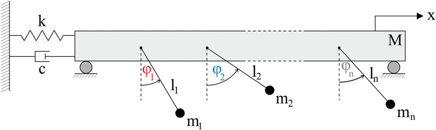
FIGURE 1. The model of n oscillating pendula with masses m_i and lengths l_i suspended on the horizontally oscillating beam. The beam of mass M is connected with the support by the spring of stiffness k and the damper of damping coefficient c. Variable x stands for displacement of the beam, while φ_i is angular displacement of i–th pendulum. The paper uncovers various types of behaviours than can be found for different sizes of the network.

The system shown in Figure 1 consists of the beam of mass M [kg], which is connected with the support by the spring of stiffness k [N/m] and the damper of damping coefficient c [Ns/m]. The beam can oscillate in the horizontal direction and its position is denoted by variable x [m]. The considered structure supports the network of n pendula (nodes) with masses m_i [kg] and lengths l_i [m], as shown in Figure 1 (i = 1, … , n). The pendula are equipped with the van der Pol type drives [32–34] (not shown in the figure) and their self–excited oscillations induce the motion of the beam, which allows to transfer the energy between the pendula. The angular displacement of the i–th node is given by variable φ_i ∈ (−π, π].

The dynamics of the system presented in Figure 1 can be investigated using the following equations of motion:

$\left\{\begin{array}{c}\left(M+\sum _{i=1}^n{m}_i\right)\ddot{x}+kx+c\dot{x}+\hfill \\ \sum _{i=1}^n{m}_i{l}_i\left({\ddot{\phi }}_i\cos {\phi }_i-{{\dot{\phi }}_i}^2\sin {\phi }_i\right)=0,\hfill \\ m_i{l}_i^2{\ddot{\phi }}_i+m_i{l}_i\ddot{x}\cos {\phi }_i+\hfill \\ c_{{\phi }_i}{\dot{\phi }}_i\left(\mu {\phi }_i^2-1\right)+m_{i}g{l}_i\sin {\phi }_i=0,\hfill \end{array}\right.(1)$

where i = 1, … , n.

During the analysis we have fixed the following parameters of system (1): M = 10 [kg] (the mass of the beam), k = 4 [N/m] (the stiffness of the spring), c = 1.53 [Ns/m] (the damping coefficient of the damper), g = 9.81 [m/s²] (the standard gravity term) and μ = 32.88 (the van der Pol type drive parameter). The damping of the i–th pendulum $c_{{\phi }_i}$ has been selected depending on the pendulum’s mass m_i and its length l_i to preserve fixed logarithmic decrement for each node.

The research presented in this paper continues the studies published in previous works [35–39]. In Refs. [35, 36] we have investigated model (1) with two nodes (n = 2), while in [37] the influence of the direction of the beam’s oscillations (horizontal, vertical and mixed) on the dynamics of two pendula has been studied. The clustering and experimental synchronization have been discussed in [38, 39], respectively.

In this paper we focus on a possible synchronization schemes for lightly supported systems, underlying the analytical solutions, which explain the observed behaviours and the results. We use the Centre-of-Mass (CoM) Theorem to show, that the performed analysis can be applied to any type of coupled oscillators arranged in a lightly supported model. The results uncovered in this paper expand the ones presented previously [35–39] and include new types of behaviours (e.g., the traveling phase solution), the appearance of the transient dynamics problems and possible multistability.

The analytical and the numerical investigations on system (1) are discussed in Section 2.

2 The results

When the beam in Figure 1 is lightly supported, i.e. k ≈ 0 [N/m] and c ≈ 0 [Ns/m], we can approximate system (1) as an isolated one. In such a case, the centre of mass of the model (the beam and the suspended pendula) is not moving, according to the Centre-of-Mass (CoM) Theorem. Consequently, the horizontal position of the centre of mass of the system shown in Figure 1 equals:

$\sigma =\frac{1}{\widehat{M}}\left(Mx+\sum _{i=1}^n{m}_i\left(x+l_i\sin {\phi }_i\right)\right)=\mathrm{c}\mathrm{o}\mathrm{n}\mathrm{s}\mathrm{t},(2)$

where $\widehat{M}=M+{\sum }_{i=1}^n{m}_i$ is the total mass of the system (the beam and the pendula).

Excluding fixed coefficient $\widehat{M}$, linearizing sin φ_i ≈ φ_i and differentiating Eq. 2 we obtain:

$\frac{\mathrm{d}\sigma }{\mathrm{d}\mathrm{t}}=M\dot{x}+\sum _{i=1}^n{m}_i\left(\dot{x}+l_i{\dot{\phi }}_i\right)=0.(3)$

Assuming similar pendula lengths l_i ≈ l = const, i = 1, … , n, one gets:

$\widehat{M}\dot{x}+\sum _{i=1}^n{m}_{i}l{\dot{\phi }}_i=0.(4)$

The solutions of Eq. 4 depend on the number of pendula n and possible synchronous configurations. To compare the analytical results obtained using Eq. 4 with the numerical simulations, we have studied networks of different size, which is presented in the following Subsections.

To physically connect the beam with the external support (see Section 1. for details), we have analyzed model (1) with parameters k = 4 [N/m] and c = 1.53 [Ns/m]. Our analysis exhibits, that such scenario can be approximated by the CoM Theorem and Eq. 4 for isolated systems, as the numerical and the analytical results match with a good precision.

2.1 The case n = 2 pendula

In this Subsection we investigate system (1) with two pendula of identical masses, i.e. m₁ = m₂ = 1.0 [kg]. The lengths of the oscillators are fixed at l₁ = 0.24848 [m] and l₂ = 0.24849 [m]. A slight difference between the lengths is used to exclude coincidental synchronization of the nodes induced by the lack of numerical differentiability. According to formula $T_i=2\pi \sqrt{l_i/g}$ [s], the natural period of each pendulum equals T ≈ 1 [s], which has been used for determining the time scales for the simulations.

Two classical solutions of model (1) with n = 2 nodes are shown in Figure 2.

FIGURE 2

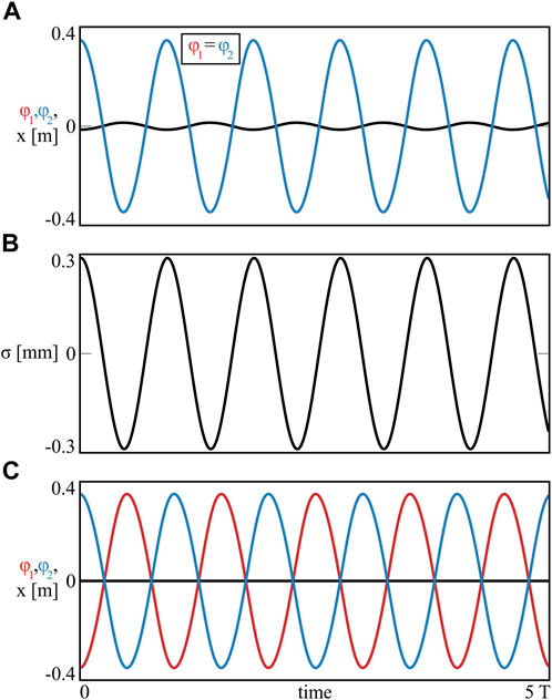
FIGURE 2. (Colour online). The in–phase synchronization of two pendula (variables φ₁, φ₂) oscillating in the anti–phase to the beam (variable x) (A) and the anti–phase synchronization of the nodes with the unmoving beam (C). The oscillations of the system’s centre of mass σ for case (A) are shown in panel (B). The results relate to classical synchronous behaviours found for coupled oscillators. System (1) with n = 2 (m₁ = m₂ = 1.0 [kg]).

Depending on the initial conditions, the pendula can stabilize on one of two possible synchronous configurations, i.e. the in–phase or the anti–phase solution.

In the first case, φ₁ = φ₂ = A sin(αt), where A [rad] and α [rad/s] denote the amplitude and the frequency of the oscillations, respectively, while t [s] is the dynamical time. For the in–phase scenario, the beam is moving, i.e. $\dot{x}\ne 0$ [m/s] and Eq. 4 allows to calculate its velocity:

$\dot{x}=-Al\alpha \left(m_1+m_2\right)\cos \left(\alpha t\right)/\widehat{M}.(5)$

Integrating Eq. 5 we obtain harmonic oscillations of the beam, with the same frequency α [rad/s] as the pendula and the anti–phase motion with respect to them. This scenario is presented in Figure 2A, where the displacements of the nodes are marked in red (φ₁) and blue (φ₂), while the movement of the beam is shown in black (x). The numerical time plots exhibit good match between the oscillations (φ₁ = φ₂) and allow to determine parameters A = 0.345 [rad] and α = 6.81 [rad/s]. The amplitude of the beam obtained from the simulations equals X_sim = 0.01412 [m], while the one calculated theoretically from Eq. 5 is given by $X_{\text{theor}}=lA(m_1+m_2)/\widehat{M}=0.01429$ [m], which shows a good match between the analytical and the numerical results. Indeed, as we have presented in Figure 2B, the centre of mass of the numerical model (the pendula and the beam considered as one system) is slightly oscillating, which is caused by the light support of the beam. As one can see, the amplitude of coefficient σ (see Eq. 2 for details) is below 0.3 [mm]. The (almost) stationary position of the centre of mass of the whole system is possible due to the movements of the beam, which oscillates in the anti–phase to the synchronized pendula as shown in Figure 2A.

The case of two pendula with equal masses includes also the anti–phase synchronous configuration, when φ₁ = A sin(αt), φ₂ = A sin(αt + π) = −A sin(αt) and the beam is not moving ($\dot{x}=0$ [m/s]). This scenario is presented in Figure 2C and can be explained using the CoM Theorem, since centre σ is stationary due to the symmetric oscillations of the nodes and the unmoving beam.

Indeed, when the beam is not moving ($\dot{x}=0$ [m/s]), Eq. 4 transforms into the following one:

$m_{1}l{\dot{\phi }}_1+m_{2}l{\dot{\phi }}_2=0.(6)$

Assuming that the pendula have synchronized with phase β ∈ [0°, 180°], i.e. φ₁ = A sin(αt) and φ₂ = A sin(αt + β), one gets from Eq. 6:

$\left\{\begin{array}{c}{m}_1+m_2\cos \beta =0,\hfill \\ m_2\sin \beta =0.\hfill \end{array}\right.(7)$

System (7) has two solutions: (i) β = 0°, when m₁ = −m₂ < 0, which is physically contradictory and (ii) β = 180°, when m₁ = m₂, which is exactly the scenario of the anti–phase synchronization shown in Figure 2C. In this case A = 0.349 [rad] and α = 6.24 [rad/s].

When the masses of the pendula in model (1) are different (m₁ ≠ m₂), one can observe also the in–phase synchronization patterns with different amplitudes and quasiperiodic motion, depending on the parameters of the system. The discussion of such scenarios can be found in [40].

2.2 The case n = 3 pendula

In this Subsection we investigate model (1) with three pendula suspended on the beam (n = 3). The lengths of the units are fixed at l₁ = 0.24848 [m], l₂ = 0.24849 [m] and l₃ = 0.2485 [m], while the masses m₁, m₂, m₃ have been varied, depending on the considered synchronous scenario.

Due to the fact, that the lengths of the pendula are almost equal, the natural periods of the oscillators remain similar and it becomes natural to assume, that the pendula can synchronize with equal amplitudes and two phases locked, i.e. φ₁ = A sin(αt), φ₂ = A sin(αt + β₂), and φ₃ = A sin(αt + β₃), where β₂, β₃ ∈ [0°, 360°) are the phases between the nodes (β₂–the phase between the 1st and the 2nd node, β₃–the phase between the 1st and the 3rd node). If $\dot{x}\approx 0$ [m/s], then Eq. 4 transforms into the following system:

$\left\{\begin{array}{c}{m}_1+m_2\cos {\beta }_2+m_3\cos {\beta }_3=0,\hfill \\ m_2\sin {\beta }_2+m_3\sin {\beta }_3=0.\hfill \end{array}\right.(8)$

System (8) consists of two equations with two variables β₂, β₃ and allows to determine the synchronous configurations (the values of the phases) when the distribution of masses m₁, m₂, m₃ is given. The examples of the behaviours observed in the considered case are shown in Figure 3.

FIGURE 3

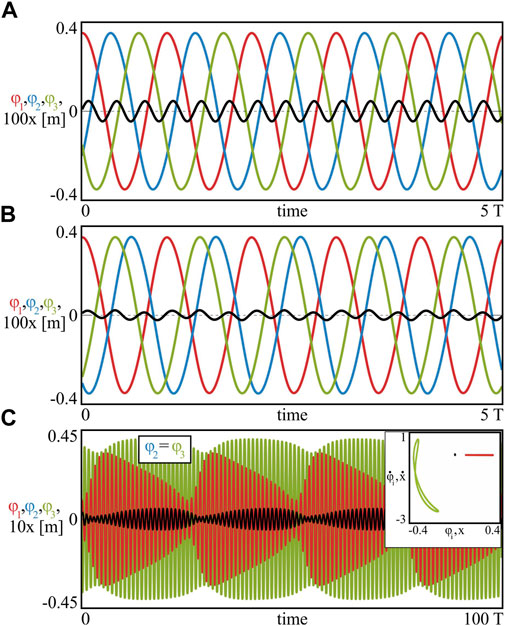
FIGURE 3. (Colour online). The periodic synchronous configurations for the identical masses (A) m₁ = m₂ = m₃ = 1.0 [kg] and non–identical masses (B) m₁ = 1.0, m₂ = 0.7, m₃ = 0.5 [kg]. The scenario of quasiperiodic synchronization between the 2nd (blue) and the 3rd (green) node is shown in panel (C) for m₁ = 1.0, m₂ = 0.5, m₃ = 0.2 [kg]. In the case of three oscillators, both regular and irregular dynamics can arise, leading to more complex synchronous scenarios. System (1) with n = 3 pendula.

The scenario of identical masses m₁ = m₂ = m₃ = 1.0 [kg] can be found in Figure 3A. The motion of the pendula has been marked in red (1st), blue (2nd) and green (3rd), while the small oscillations of the beam are shown in black (the latter time plot is multiplied 100 times–100x). Assuming that the velocity of the beam’s oscillations is small compared to the pendula, we can apply system (8) for finding the attractors. Indeed, Eq. 8 for m₁ = m₂ = m₃ = 1.0 [kg] have two solutions: (i) β₂ = 120°, β₃ = 240°and (ii) β₂ = 240°, β₃ = 120°, which indicate the same state, since the masses of the pendula are equal. The example of the phase–locked synchronization pattern shown in Figure 3A corresponds to analytical result (i), with the phases calculated numerically at β₂ = 120.21°and β₃ = 240.68°. The centre of mass of the system is almost stationary, with the amplitude of its oscillations equal to A_σ = 3.17 ⋅ 10^–6 [m].

When the pendula are non–identical, the values of phases β₂, β₃ strictly depend on the distribution of the masses and possible solutions of system (8). The example of the phase–locked state for m₁ = 1.0, m₂ = 0.7 and m₃ = 0.5 [kg] is presented in Figure 3B, where the numerical values of the phases equal β₂ = 207.63°, β₃ = 139.08°. The analytical solution that can be obtained using Eq. 8 matches with the numerical one, exhibiting phases β₂ = 207.72°and β₃ = 139.32°. In this case, the amplitude of the centre of mass does not exceed A_σ = 2.62 ⋅ 10^–6 [m]. It should be noted, that one can observe also the second synchronous configuration, for which β₂ = 152.37°and β₃ = 220.92°. The appearance of the pair of phase–locked states is associated with the following property of system (8): if $({\beta }_2^{*},{\beta }_3^{*})$ is the solution of Eq. 8, then (360 °- ${\beta }_2^{*},360$ °- ${\beta }_3^{*}$) is also the solution of (8).

The pendula of model (1) can also synchronize in the in–phase, similar to n = 2 scheme (see Section 2.1. for details). In this case, the applicability of system (8) is excluded, since the beam is oscillating against the pendula (to keep the centre of mass stationary) and consequently $\dot{x}\ne 0$ [m/s]. Depending on the parameters, both the in–phase and the phase–locked solutions can co–exist, which has been shown in Figure 4A.

FIGURE 4

FIGURE 4. (Colour online). The basins of attraction for different distribution of the pendula masses. In (A) the scenario of three co–existing periodic synchronous states is shown (IN: in–phase state, PL: the first phase–locked state and PL*: the second phase–locked state), while in (B) the case of bi–stability of the in–phase (IN) and the quasiperiodic (Q) configurations is presented. The values of the masses in panels (A) and (B) correspond to the ones considered in Figure 3B and Figure 3C, respectively. The results show, that depending on the initial conditions, various types of behaviours co–exist.

The results presented in Figure 4A correspond to the case of m₁ = 1.0, m₂ = 0.7, m₃ = 0.5 [kg] (see the time plots in Figure 3B) and uncover the basins of attraction of three possible solutions: 1) the in–phase synchronization (IN–yellow), 2) the first phase–locked configuration with β₂ = 152.37°, β₃ = 220.92°(marked as PL–dark blue) and 3) the second phase–locked configuration with β₂ = 207.72°, β₃ = 139.32°(marked as PL*–light blue; to distinguish that the observed phase–locked solutions are different in the sense of β₂, β₃ phases distribution, we denote the second state by asterisk). The basins in Figure 4A are shown in subspace (φ₂, φ₃) ∈ (−π,π]² (the initial positions of the 2nd and the 3rd pendulum), with the remaining conditions fixed at zeros, i.e. $x,\dot{x},{\phi }_1,{\dot{\phi }}_1,{\dot{\phi }}_2,{\dot{\phi }}_3=0$. The structure of the basins indicates, that the prediction of the final synchronous solution can become not straightforward, when the precision of the initial state is insufficient.

As we have shown, the analytical solutions of system (8) for the chosen distribution of the pendula masses indicate possible attractors of model (1) with a good precision (differences between the analytical and the numerical phases β₂, β₃). Moreover, it can be easily shown, that for particular masses m_i, i = 1, 2, 3, system (8) may not have any solution, which suggests the disappearance of phase–locked configurations. The example of such scenario is discussed in Figure 3C and Figure 4B for m₁ = 1.0, m₂ = 0.5 and m₃ = 0.2 [kg]. Due to the fact, that Eq. 8 have no solution for the chosen masses, the oscillations of the pendula shown in Figure 3C become quasiperiodic and grouped into two clusters: 1) the 1st pendulum (red; φ₁) and 2) the quasiperiodic, synchronous motion of the 2nd and the 3rd node (blue and green; φ₂ = φ₃). The quasiperiodic character of the vibrations has been confirmed using Poincare sections, which are included in the inbox in Figure 3C. The 1st (red) pendulum has been chosen as the reference node for creating the maps, i.e. the points have been collected every time it reached the local maximum. The observed quasiperiodic state co–exists with the in–phase synchronization and the basins of these two possible behaviours are shown in Figure 4B (the in–phase state–I in yellow; the quasiperiodic state–Q in brown). It should be noted, that the almost stationary position of the centre of mass in the case of quasiperiodic oscillations is preserved, with the amplitude A_σ = 1.2 ⋅ 10^–4 [m].

To investigate possible transitions between different synchronous configurations of model (1) with n = 3 pendula, we have performed the bifurcation analysis in relation to system (8). The example of the bifurcation scenario for fixed masses m₁ = 1.0, m₂ = 0.5 [kg] and varied m₃ is shown in Figure 5.

FIGURE 5

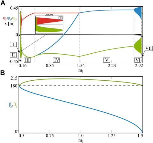
FIGURE 5. (Colour online). The bifurcation diagrams of model (1) for fixed m₁ = 1.0, m₂ = 0.5 [kg] and varied m₃ ∈ [0.16, 2.92] [kg] (A). The interval is split into seven cases (I–VII), depending on the behaviour of the pendula and possible solutions of system (8). The bifurcations of phases β₂ and β₃ corresponding to the phase–locked synchronous configurations during stage IV are shown in panel (B). Using bifurcation analysis, one can trace transitions occurring in the system and the arise of different types of states.

The bifurcation diagrams shown in Figure 5A are split into seven regions: I–VII, depending on the dynamics of the pendula and possible synchronous configurations. The procedure applied for collecting the points for the diagrams is the same as the one used for the Poincare section shown in the inbox in Figure 3C (the 1st pendulum is chosen as the reference one).

The analysis begins at m₃ = 0.2 [kg], when the behaviour of the system is quasiperiodic as shown in Figure 3C. This type of dynamics can be observed in a narrow region labelled as II for 0.1885 < m₃ < 0.2158 [kg], which has been enlarged in the inbox in Figure 5A. Decreasing the mass of the 3rd pendulum, at m₃ = 0.1885 [kg] the system bifurcates into region I, where all three pendula synchronize in the in–phase. Further decrease of parameter m₃ does not change the dynamics of the model, since the synchronized pendula act as one clustered node, which oscillates in the anti–phase to the beam of a fixed mass. In both regions I and II, system (8) has no solutions.

Bifurcating model (1) in the opposite direction, i.e. starting from case II for m₃ = 0.2 [kg] and increasing parameter m₃, one can observe the vanishing of the quasiperiodic solution, which finally bifurcates into the periodic one for m₃ = 0.2158 [kg] (region III). In this case, the 2nd (blue) and the 3rd (green) pendula are still synchronized (forming a cluster) but the amplitude of their oscillations is greater than the amplitude of the 1st (red) node. This scenario corresponds to the case of two pendula with different masses, which synchronize with various amplitudes [35, 40]. The reported dynamics resides in region III for 0.2158 ≤ m₃ < 0.5 [kg], where the relation m₁ > m₂ + m₃ is satisfied. With the increase of mass m₃, the amplitude of the clustered pendula (blue and green) also increases and finally reaches the amplitude of the red node at m₃ = 0.5 [kg], when m₁ = m₂ + m₃. The system bifurcates into stage IV, where all of the pendula are oscillating with the same amplitude and system (8) has two analytical solutions leading to the phase–locked synchronous states. The phases between the pendula (β₂, β₃) observed in this scenario are shown in Figure 5B for 0.5 ≤ m₃ ≤ 1.5 [kg]. In the beginning of stage IV, for m₃ = 0.5 [kg] the phases are equal: β₂ = β₃ = 180°; this corresponds to the anti–phase pattern between the clustered nodes (blue and green) and the solitary one (red), since m₁ = m₂ + m₃. With the increase of mass m₃, the cluster breaks as the 2nd pendulum begins to converge to the 1st one (β₂ decreases as shown in Figure 5B). The system resides on the phase–locked attractor with the phases depending on the value of m₃. The convergence of the blue node to the red one is continued in a wide range of parameter m₃, until the critical point at m₃ = 1.5 [kg], for which β₂ = 0°and β₃ = 180°. In this scenario the 1st (red) and the 2nd (blue) pendula clustered, leaving the 3rd (green) one solitary. The synchronization becomes anti–phase, according to equality m₁ + m₂ = m₃.

With further increase of mass m₃, the system bifurcates into stage V, where Eq. 8 have no solutions and the pendula oscillate with different amplitudes. For 1.5 < m₃ < 2.732 [kg] (region V), the amplitude of the clustered nodes (red and blue) is higher than the one observed for the 3rd (green) pendulum, as m₁ + m₂ < m₃. The scenario changes from periodic to quasiperiodic motion for m₃ = 2.732 [kg], when the dynamics reaches region VI. In this case, the clustered character of the pendula is preserved, as shown in the diagram in Figure 5A. With further increase of mass m₃ [kg], the model finally stabilizes on the in–phase synchronization pattern for m₃ ≥ 2.887 [kg], which has been labelled as region VII.

Scenarios I and VII are qualitatively the same. In scenarios (II and VI) and (III and V) one can observe the clustering of the pendula and their quasiperiodic or periodic dynamics, respectively. The clustering configuration depends on the distribution of masses m₁, m₂, m₃ and one can obtain different patterns varying these parameters. The remaining case IV allows to observe phase–locked synchronous motion, which can be described by the analysis of the centre of mass, i.e. system (8).

To examine possible phase–locking patterns between the pendula, we have investigated Eq. 8 for fixed mass m₁ = 1.0 [kg] and varied m₂, m₃. Our results are presented in Figure 6.

FIGURE 6

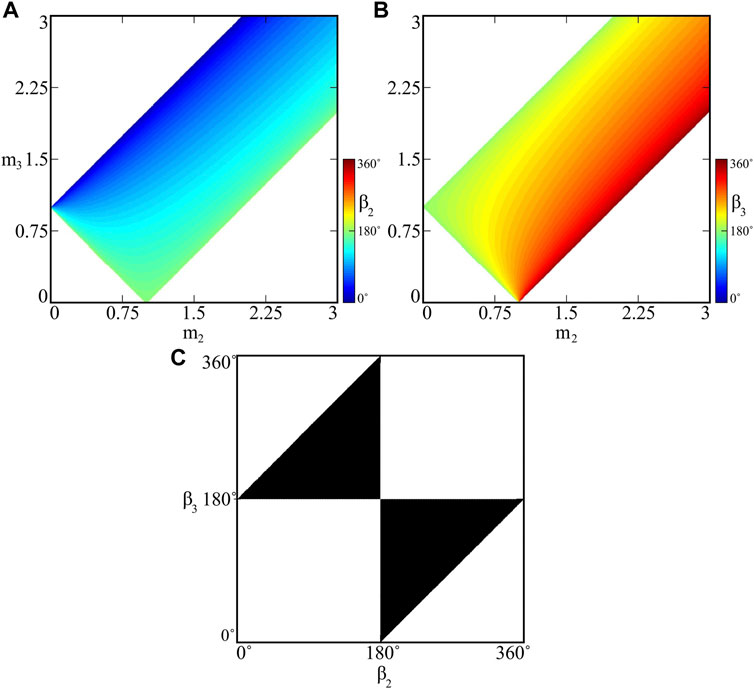
FIGURE 6. (Colour online). The values of the phases within the phase–locked synchronization patterns for fixed m₁ = 1.0 [kg] and varied m₂, m₃: values of β₂ and β₃ are shown in panels (A) and (B), respectively. The possible phases β₂, β₃, which can be realized by model (1) due to the solvability of system (8) are shown in (C). The results determine regions, where particular types of behaviours can be found, as well as their properties.

In Figures 6A,B one can see the values of phases β₂ (panel a) and β₃ (panel b) obtained analytically using system (8) for m₂, m₃ ∈ [0, 3] [kg] (mass m₁ = 1.0 [kg] fixed). The results have been limited to the case, when β₂ ∈ [0, 180°] (as described above, system (8) has a pair of solutions, i.e. (β₂, β₃) and (360° − β₂, 360° − β₃)). Using the maps presented in Figures 6A,B one can identify the regions of the pendula masses, for which phase–locked synchronization is possible. We have also calculated analogous maps by the numerical examination of model (1) for m₂, m₃ ∈ [0, 3] [kg] and the obtained results (phases) match with the ones observed for the analytical case. It should be noted, that the regions left blank in Figures 6A,B correspond to the in–phase synchronization and/or quasiperiodic motion, depending on the parameters.

The relation between the pendula masses m_i, i = 1, 2, 3 and phases β₂, β₃ can be also inverted, i.e. one can investigate what values of the masses should be selected for the desired phase–locked configuration (particular values of the phases). Indeed, fixing the mass of a selected pendulum, e.g. m₁ and considering β₂, β₃ as the parameters, we can calculate the values of the remaining masses m₂ and m₃ from Eq. 8 in the following way:

$\left\{\begin{array}{c}{m}_2=\frac{-m_1\sin {\beta }_3}{\sin \left({\beta }_3-{\beta }_2\right)},\hfill \\ m_3=\frac{m_1\sin {\beta }_2}{\sin \left({\beta }_3-{\beta }_2\right)}.\hfill \end{array}\right.(9)$

Using Eq. 9 one can calculate the values of m₂ and m₃, which allow to obtain the desired (β₂, β₃) phase–locked synchronous configuration. The solutions of (9) have the physical sense only when both formulas are greater than zero; the regions of (β₂, β₃) values corresponding to such scenario are shown in Figure 6C in black. The presented map allows to determine which values of the phases (the ones corresponding to the black domain) can be realized by system (1) within the phase–locked state. It should be noted, that close to the borders of the region shown in Figure 6C, masses m₂, m₃ in Eq. 9 converge to zero or infinity, which may influence the dynamics of system (1) and lead to unexpected behaviours.

2.3 The case n = 4 pendula

In this Subsection we study the case of model (1) with four pendula suspended on the beam (n = 4). The lengths of the oscillators are chosen as l₁ = 0.24848 [m], l₂ = 0.24849 [m], l₃ = 0.2485 [m] and l₄ = 0.24851 [m]. If the pendula synchronize with equal amplitudes and phases locked, i.e. φ_i = A sin(αt + β_i), i = 1, 2, 3, 4, where β₁ = 0°and β₂, β₃, β₄ ∈ [0°, 360°), then for $\dot{x}\approx 0$ [m/s] (the beam slightly oscillating) Eq. 4 transforms into the following system:

$\left\{\begin{array}{c}{m}_1+m_2\cos {\beta }_2+m_3\cos {\beta }_3+m_4\cos {\beta }_4=0,\hfill \\ m_2\sin {\beta }_2+m_3\sin {\beta }_3+m_4\sin {\beta }_4=0.\hfill \end{array}\right.(10)$

Depending on the values of masses m_i, i = 1, 2, 3, 4, system (10) can have no solutions or infinitely many solutions (two equations with three variables β₂, β₃, β₄). The considered scenario is more complex than the one observed for n = 3 pendula, where the number of solutions of Eq. 8 has been limited (see Section 2.2. for details).

To investigate model (1) with four nodes, we have varied pendula masses in different scenarios. The examples of possible dynamical patterns are discussed in Figure 7.

FIGURE 7

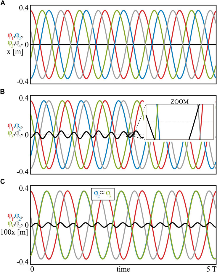
FIGURE 7. (Colour online). Possible behaviours of the pendula for (A) m₁ = m₂ = m₃ = m₄ = 1.0 [kg] (identical masses and the traveling phase state), (B) m₁ = 1.0, m₂ = 0.99, m₃ = 1.01, m₄ = 0.985 [kg] (slightly different masses and the phase–locked state) and (C) m₁ = 1.0, m₂ = 0.7, m₃ = 0.5, m₄ = 0.45 [kg] (different masses and the clustering of the pendula). System (1) with n = 4 nodes. In the case of four coupled pendula, one can identify new types of states and even more complex synchronous scenarios.

We have investigated three main schemes of the masses distribution, i.e. identical masses, slightly different masses and different masses, which are discussed below.

If the pendula are identical, i.e. m_i = const, i = 1, 2, 3, 4, then system (10) can be simplified by dividing the equations by the masses. It can be easily shown, that in such scenario, the solutions of (10) are given as follows: β₂ = 180°, ${\beta }_3=\widehat{\beta }$ and ${\beta }_4=\widehat{\beta }+180$°, where $\widehat{\beta }\in [0°,360°)$ becomes the parameter of system (10) (the order of the values of phases β₂, β₃ and β₄ can be arbitrarily chosen since the pendula are identical). In this case, system (10) indicates infinitely many phase–locked synchronous states along parameter $\widehat{\beta }\in [0°,360°)$, within which pendula form two clusters: 1) the cluster of the 1st and the 2nd pendulum oscillating in the anti–phase and 2) the cluster of the 3rd and the 4th pendulum also oscillating in the anti–phase. The phase shift between the clusters is given by parameter $\widehat{\beta }$, which also determines the phase between the 1st and the 3rd pendulum.

The example of the described scenario is presented in Figure 7A for m₁ = m₂ = m₃ = m₄ = 1.0 [kg], where the time plots of the nodes are marked in red (1st), blue (2nd), green (3rd), and grey (4th), while the beam is shown in black. Since the oscillations within the clusters are anti–phase (red vs. blue and green vs. grey), the beam is not moving (as have been described previously for n = 2 pendula in Figure 2C; see Section 2.1. for details). As we have observed, the phase between the clusters (parameter $\widehat{\beta }$) changes continuously with time, leading to the solution, which can be called the “traveling phase” state. The traveling character of the observed configuration is shown in Figure 8A.

FIGURE 8

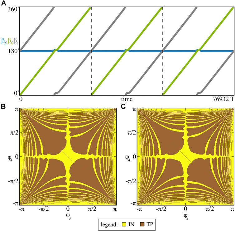
FIGURE 8. (Colour online). In (A) the traveling of phases β₂, β₃ and β₄ for identical pendula m_i = 1.0 [kg], i = 1, 2, 3, 4 is shown. The basins of attraction of possible dynamical patterns (IN and TP) for varied (φ₃, φ₄) ∈ (−π,π]² and (φ₂, φ₄) ∈ (−π,π]² are presented in panels (B) and (C), respectively. The arise of the traveling phase state is related to the similarities in the pendula properties (the masses).

The diagrams included in Figure 8A present the values of β₂, β₃ and β₄ phases in a long time interval of model (1) simulations. As one can see, the numerical solution matches with the analytical one (β₂ = 180°, ${\beta }_3=\widehat{\beta }$, ${\beta }_4=\widehat{\beta }+180$°) and the configuration of the clusters (the 1st and the 2nd pendulum clustered; the 3rd and the 4th pendulum clustered) is preserved, except for short disruptions around β₃ = 180°, when the clusters overlap in the phase space. The results shown in Figure 8A include three cycles of phase traveling, which has been indicated by the vertical, dashed lines; the approximated length of one full cycle equals 25 644 T.

As we have observed during various simulations, the configuration of the clusters can be correlated with the lengths of the pendula, i.e. the slight differences in lengths l_i and their distribution within the nodes determine the pairs, which will cluster. For the considered l₁ = 0.24848 [m], l₂ = 0.24849 [m], l₃ = 0.2485 [m] and l₄ = 0.24851 [m], system (1) has always finally converged to the scenario shown in Figure 8A and the observed clustering has been independent of the initial conditions. The described property has not been observed when varying the conditions from and between the clusters, which has been shown in Figures 8B,C for the basins of attraction. The scenarios of varied (φ₃, φ₄) ∈ (−π,π]² and (φ₂, φ₄) ∈ (−π,π]² (the remaining conditions equal to zeros) are presented in Figure 8B and Figure 8C, respectively and correspond to the initial conditions of the pendula forming the cluster (b) and the initial conditions of the pendula from different clusters (c). As one can see, the “traveling phase” state (TP, brown) co–exists with the in–phase synchronization pattern (IN, yellow) but the regions of convergence for both scenarios (b) and (c) are qualitatively indifferent.

The traveling character of the phases between the pendula is possible due to the identity of the masses. When the masses become slightly different, system (10) cannot be simplified as previously but its solutions are close to the ones described above (two clusters), since m₁ ≈ m₂ ≈ m₃ ≈ m₄. The example of such scenario is shown in Figure 7B for m₁ = 1.0, m₂ = 0.99, m₃ = 1.01, m₄ = 0.985 [kg]. As one can see, the 1st (red) and the 4th (grey) pendulum are synchronized almost in the anti–phase (the first cluster) and the 2nd (blue) and the 3rd (green) pendulum are also synchronized close to the anti–phase state (the second cluster). The slight shifts in the oscillations of the pendula within the clusters are shown in the enlargement in Figure 7B. Since the motion is not precisely anti–phased, the beam exhibits slight oscillations, which magnitude has been increased 1000 times for better clarity (1000x in the figure).

The slight differences in the masses of the pendula lead to the disappearance of the TP state and stabilization of the nodes on particular phase–locked synchronous configuration. The example of the evolution of phases β₂, β₃ and β₄ for such scenario is presented in Figure 9A.

FIGURE 9

FIGURE 9. (Colour online). The evolution of phases β₂, β₃, β₄ (left panel) and possible synchronous configurations in (β₂, β₃) plane (right panel). Results (A,B) correspond to the case of slightly different masses: m₁ = 1.0, m₂ = 0.99, m₃ = 1.01, m₄ = 0.985 [kg], while results (C,D) have been obtained for different masses m₁ = 1.0, m₂ = 0.7, m₃ = 0.5, m₄ = 0.45 [kg]. The results exhibit, that the distribution of the pendula masses plays a major role in possible behaviours of the system.

The points for the diagrams included in Figure 9A have been collected after 1000 T [s], which has been considered as possible transient time for the stabilization of the system. As one can see, the time necessary for the full stabilization has reached around 500 000 T [s], as the phases are changing for a long time interval (time below 250 000 T [s] in Figure 9A). Our analysis for various initial conditions exhibits, that for slightly different masses of the pendula, system (1) finally converges to particular phase–locked state but the transient time of such stabilization can become very long (even exceeding 500 000 T [s]). These results uncover possible transient dynamics problems [41–43], which can arise when studying complex networks and become misleading for the researcher trying to determine the attractor(s) of the considered model.

As we have described above, system (10) can have infinitely many solutions for the fixed masses, leading to the possibility of the infinitely many phase–locked configurations. To investigate this property for the considered slightly different masses, we have performed a series of trials, simulating model (1) from random initial conditions and determining the final synchronous configuration. The results of our analysis are discussed in Figure 9B and are based on 1000 trials in total.

For each numerical trial we have simulated system (1) for 500 000 T [s], after which the observed pattern has been examined for stability (if the phases β₂, β₃ and β₄ are still changing or not). In the case of the stable phases, the obtained phase–locked configuration has been included in Figure 9B in the form of the red dot, which coordinates indicate values β₂ (horizontal axis) and β₃ (vertical axis), while the dot’s label (in grey text) equals the value of phase β₄. As one can see, the points marked in Figure 9B exhibit linear relation (the dashed red line along the points) and the values of the obtained phases are close to the solution, which can be calculated from system (10) for the identical masses, i.e. β₄ ≈ 180°, ${\beta }_2=\widehat{\beta }$ and ${\beta }_3\approx \widehat{\beta }+180$°(the order is determined by the distribution of the slightly different masses).

To prevent the overlapping of the states, when the phases β₂, β₃ and β₄ for two particular trials are slightly different (which may be caused by numerical inaccuracies), we have applied the following criterion for distinguishing the states: “Configuration 1” with phases ${\beta }_2^{1*}$, ${\beta }_3^{1*}$, ${\beta }_4^{1*}$ is considered as different from “Configuration 2” with phases ${\beta }_2^{2*}$, ${\beta }_3^{2*}$, ${\beta }_4^{2*}$ when $\left|{\beta }_2^{1*}-{\beta }_2^{2*}\right|>\delta$, $\left|{\beta }_3^{1*}-{\beta }_3^{2*}\right|>\delta$ and $\left|{\beta }_4^{1*}-{\beta }_4^{2*}\right|>\delta$, where parameter δ determines the chosen accuracy. The results included in Figure 9B have been obtained for δ = 1.8°, i.e. 1/200–th of the full angle. As we have observed, by loosening the criterion (decreasing the value of coefficient δ), the number of the points increases, filling the dashed red line in Figure 9B. The described observation suggests, that when the masses of the pendula are slightly different, system (1) can produce many stable co–existing phase–locked synchronous configurations (according to Eq. 10 and their possible stable solutions), converging to the case of even extreme multistability [28–30] when the differences in the masses become shrinked.

In the last considered scenario we have studied model (1) with different masses, fixing m₁ = 1.0, m₂ = 0.7, m₃ = 0.5 and m₄ = 0.45 [kg]. The phase–locked pattern obtained for the given distribution is shown in Figure 7C, where the 2nd (blue) and the 3rd (green) pendulum formed the cluster (φ₂ ≈ φ₃) and the scenario is similar to the one observed for n = 3 coupled nodes (see Section 2.2. for details). Indeed, when the masses of the pendula are different, the system (apart from the in–phase synchronization) tends to the clustering of the nodes [44–47]. This property has been also observed for larger networks, when the oscillators group into three clusters [38].

In the case of clustering, possible phases between the pendula can be easily obtained using CoM Theorem and system (10). Indeed, when two of the pendula form a cluster, e.g. the 3rd and the 4th, we obtain φ₃ = φ₄, β₃ = β₄ and the simplification of Eq. 10 in the following form:

$\left\{\begin{array}{c}{m}_1+m_2\cos {\beta }_2+\left(m_3+m_4\right)\cos {\beta }_{34}=0,\hfill \\ m_2\sin {\beta }_2+\left(m_3+m_4\right)\sin {\beta }_{34}=0,\hfill \end{array}\right.(11)$

where β₃₄ = β₃ = β₄. The above system is analogous to system (8) for n = 3 pendula and possesses solutions depending on the values of m₁, m₂ and (m₃ + m₄).

For four pendula one can obtain six different configurations of clustering (m₁ + m₂, m₁ + m₃, m₁ + m₄, m₂ + m₃, m₂ + m₄ and m₃ + m₄), of which three lead to solutions of system (10) for the considered masses m₁ = 1.0, m₂ = 0.7, m₃ = 0.5 and m₄ = 0.45 [kg]. Each clustering configuration involves a pair of phase–locked synchronous solutions (see Section 2.2. for details), which results in six different synchronization patterns in total. The latter ones have been listed as “phase–locking (1)–(6)” in Table 1, where in the first column the labels of the states are shown (attractor type), while in the second one the values of the phases obtained analytically from (10) are presented (analytical phases). The table includes also the in–phase synchronization pattern and the “phase–locking (*)” state, which is discussed further.

TABLE 1

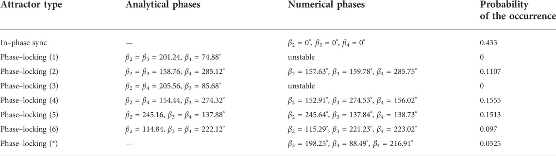
TABLE 1. The comparison of the analytical and the numerical phases for the phase–locked synchronous configurations (1)–(6). The probabilities of the occurrence of possible states are given in the last column. System (1) with different masses: m₁ = 1.0, m₂ = 0.7, m₃ = 0.5, m₄ = 0.45 [kg].

The example of the phases convergence for “phase–locking (2)” state is included in Figure 9C and shows the evolution of phases β₂, β₃ and β₄ for 50 000 T [s] (the points collected after 1000 T [s]). In this case, the phases stabilize faster than for the slightly different masses scenario (compare Figure 9A and Figure 9C) and the transient motion becomes easier to omit. The phases of the 2nd (blue, β₂) and the 3rd (green, β₃) node are very similar, which exhibits a good match between the analytical results and the ones obtained from the numerical simulations. The comparison of both cases can be found in Table 1 in the second (analytical phases) and the third (numerical phases) columns.

As one can see in Table 1, two patterns “phase–locking (1)” and “phase–locking (3)” are labelled as unstable. Even though system (10) can have particular solution (e.g., the “phase–locking (1)”state), its stability has to be examined numerically by simulating the model. To investigate the attractors of system (1) for different masses, we have performed a series of 40 000 trials, determining the synchronous configurations after 10 000 T [s]. The obtained results are discussed in Figure 9D in (β₂, β₃) plane, with the values of β₄ labeling the points (see also the description of Figure 9B above). Four black dots correspond to solutions “phase–locking (2), (4), (5) and (6)” described in Table 1, while the single red dot indicates the solution “phase–locking (*)” (the last row in Table 1), for which the pendula have not clustered. During the simulations we have not observed the stability of patterns “phase–locking (1)” and “phase–locking (3)”, which suggest that these solutions are unstable. It should be noted though, that the phases obtained for the “phase–locking (*)” state are close to the analytical ones for “phase–locking (3)”, which may indicate that these configurations are closely related and the difference between the analytics and the numerics results from the assumptions of the considered model (not completely isolated).

The probability analysis performed for the solutions included in Table 1 shows, that the in–phase synchronous configuration is the most probable state (probability around 43%), while the phase–locked patterns appear with similar probabilities ranging from 5% to 15%. The presented results are based on a series of 40 000 trials as mentioned above; for each trial, the initial positions of the pendula have been sampled from the uniform distribution U[ − π, π), with the remaining initial conditions of the system considered zeros.

It should be noted, that the considered scenario of four coupled pendula includes also other possible behaviours, such as quasiperiodic dynamics or synchronous patterns with different amplitudes. When the pendula group into three clusters (as shown in Figure 7C), the scenario is analogous to the synchronization of three oscillators (n = 3 in Section 2.2.) and we can perform similar bifurcation analysis as the one presented in Figure 5.

Generalizing the results, when model (1) consists of n > 4 pendula synchronized within the phase–locked state, i.e. φ_i = A sin(αt + β_i), i = 1, … , n, β₁ = 0°and β₂, … , β_n ∈ [0°, 360°), system (4) transforms into the following equations:

$\left\{\begin{array}{c}{m}_1+\sum _{i=2}^n{m}_i\cos {\beta }_i=0,\hfill \\ \sum _{i=2}^n{m}_i\sin {\beta }_i=0.\hfill \end{array}\right.(12)$

System (12) can possess infinitely many solutions and generalizes system (10) considered for n = 4 nodes. In this case, one can expect to obtain similar synchronous configurations and dynamics, depending on the parameters of the pendula and the beam, as well as the initial conditions. The increased number of nodes can lead to the appearance of more complex behaviours, including chimeras [48, 49] and chimera–like states [50, 51], which occur naturally in the networks of coupled oscillators.

3 Conclusion

In this paper we have investigated the dynamics of coupled self–excited pendula, arranged in a lightly supported system. Depending on the network’s size (the number of the nodes suspended on the beam), one can observe different types of synchronous configurations and behaviours. Our results are based on the Centre-of-Mass (CoM) Theorem, which can be applied to the considered, almost isolated system. We have described typical dynamical structures, including the in–phase and the anti–phase synchronization, as well as more complex patterns like the clustering of the pendula or the phase–locked solutions. The basins of attraction included in the study uncover possible co–existence configurations of the system’s states, while the bifurcation analysis allows to trace the transitions between different synchronous solutions. The analysis can be further applied for determining the relations between the pendula masses and their phases within the phase–locking scenarios, which has been included in the results. During the research we have uncovered the “traveling phase” state, which is characterized by the continuous change of the phases between the synchronized oscillators and transient dynamics problems, leading to the uncertainty about the stabilization of the observed synchronous states. The analysis of the considered models has exhibited possible high multistability with many co–existing attractors, that can be observed for slightly different nodes.

The analytical results obtained from the CoM Theorem match with the numerical ones calculated during simulations. The former results explain and allow to understand the dynamics that is observed within the models, especially the synchronous configurations between the pendula. As we have shown, the theory approximates lightly supported systems with a good precision and can be applied for studying similar networks of the mechanical type. The latter can be especially beneficial in the case of experimental investigations, since the structure of presented model allows to confirm the results practically with the use of simple mechanical setup.

Data availability statement

The raw data supporting the conclusion of this article will be made available by the authors, without undue reservation.

Author contributions

All authors listed have made a substantial, direct, and intellectual contribution to the work and approved it for publication.

Funding

This work has been supported by the National Science Centre, Poland: SONATA Programme (Project No 2019/35/D/ST8/00412) and OPUS Programmes (Project No 2018/29/B/ST8/00457 and Project No 2021/43/B/ST8/00641).

Conflict of interest

The authors declare that the research was conducted in the absence of any commercial or financial relationships that could be construed as a potential conflict of interest.

Publisher’s note

All claims expressed in this article are solely those of the authors and do not necessarily represent those of their affiliated organizations, or those of the publisher, the editors and the reviewers. Any product that may be evaluated in this article, or claim that may be made by its manufacturer, is not guaranteed or endorsed by the publisher.

References

1. Pikovsky A, Rosenblum M, Kurths J. Synchronization: A universal concept in nonlinear sciences. Cambridge University Press (2003).

Google Scholar

2. Blekhman II. Synchronization in science and technology. American Society of Mechanical Engineers (ASME) (1988).

Google Scholar

3. Nijmeijer H, Rodriguez-Angeles A. Synchronization of mechanical systems. World Scientific (2003).

Google Scholar

4. Awerbuch B. Complexity of network synchronization. J ACM (1985) 32(4):804–23. doi:10.1145/4221.4227

CrossRef Full Text | Google Scholar

5. Arenas A, Diaz-Guilera A, Kurths J, Moreno Y, Zhou C. Synchronization in complex networks. Phys Rep (2008) 469(3):93–153. doi:10.1016/j.physrep.2008.09.002

CrossRef Full Text | Google Scholar

6. Ghosh D, Frasca M, Rizzo A, Majhi S, Rakshit S, Alfaro-Bittner K, et al. The synchronized dynamics of time-varying networks. Phys Rep (2022) 949:1–63. doi:10.1016/j.physrep.2021.10.006

CrossRef Full Text | Google Scholar

7. Barahona M, Pecora LM. Synchronization in small-world systems. Phys Rev Lett (2002) 89:054101. doi:10.1103/physrevlett.89.054101

PubMed Abstract | CrossRef Full Text | Google Scholar

8. Nair S, Leonard NE. Stable synchronization of mechanical system networks. SIAM J Control Optim (2008) 47(2):661–83. doi:10.1137/050646639

CrossRef Full Text | Google Scholar

9. Mahmoud GM, Aly SA, Al-Kashif MA. Dynamical properties and chaos synchronization of a new chaotic complex nonlinear system. Nonlinear Dyn (2008) 51:171–81. doi:10.1007/s11071-007-9200-y

CrossRef Full Text | Google Scholar

10. Boccaletti S, Kurths J, Osipov G, Valladares DL, Zhou CS. The synchronization of chaotic systems. Phys Rep (2002) 366(1):1–101. doi:10.1016/s0370-1573(02)00137-0

CrossRef Full Text | Google Scholar

11. Ver Hoeye S, Suarez A, Sancho S. Analysis of noise effects on the nonlinear dynamics of synchronized oscillators. IEEE Microw Wirel Compon Lett (2001) 11(9):376–8. doi:10.1109/7260.950766

CrossRef Full Text | Google Scholar

12. Spong MW, Chopra N. Synchronization of networked Lagrangian systems. In: Lagrangian and Hamiltonian methods for nonlinear control 2006. Springer Berlin Heidelberg (2007). p. 47.

Google Scholar

13. Borhaug E. Nonlinear control and synchronization of mechanical systems (Doctoral thesis). Norway: Norwegian university of science and technology (2008).

Google Scholar

14. De Sousa Vieira M, Lichtenberg AJ, Lieberman MA. Nonlinear dynamics of self-synchronizing systems. Int J Bifurcation Chaos (1991) 1(3):691–9. doi:10.1142/s0218127491000506

CrossRef Full Text | Google Scholar

15. Fang P, Hou Y. Synchronization characteristics of a rotor-pendula system in multiple coupling resonant systems. Proc Inst Mech Eng C: J Mech Eng Sci (2018) 232(10):1802–22. doi:10.1177/0954406217711468

CrossRef Full Text | Google Scholar

16. Baker GL, Blackburn JA, Smith HJT. Intermittent synchronization in a pair of coupled chaotic pendula. Phys Rev Lett (1998) 81:554–7. doi:10.1103/physrevlett.81.554

CrossRef Full Text | Google Scholar

17. Ramirez JP, Alvarez J. Rotating waves in oscillators with Huygens’ coupling**This work was partly supported by the CONACyT under Grant CB2012-180011-Y. IFAC-PapersOnLine (2015) 48(18):71–6. doi:10.1016/j.ifacol.2015.11.013

CrossRef Full Text | Google Scholar

18. Pogromsky AY, Belykh VN, Nijmeijer H. Controlled synchronization of pendula. In: 42nd IEEE International Conference on Decision and Control (IEEE Cat. No.03CH37475), 5 (2003). p. 4381.

Google Scholar

19. Fradkov AL, Andrievsky B, Ananyevskiy M. State estimation and synchronization of pendula systems over digital communication channels. Eur Phys J Spec Top (2014) 223(4):773–93. doi:10.1140/epjst/e2014-02140-0

CrossRef Full Text | Google Scholar

20. Mendes RV. Multistability in dynamical systems. World Scientific (1999). p. 105.

Google Scholar

21. Feudel U. Complex dynamics in multistable systems. Int J Bifurcation Chaos (2008) 18(06):1607–26. doi:10.1142/s0218127408021233

CrossRef Full Text | Google Scholar

22. Li C, Hu W, Sprott JC, Wang X. Multistability in symmetric chaotic systems. Eur Phys J Spec Top (2015) 224:1493–506. doi:10.1140/epjst/e2015-02475-x

CrossRef Full Text | Google Scholar

23. Brzeski P, Perlikowski P. Sample-based methods of analysis for multistable dynamical systems. Arch Comput Methods Eng (2019) 26:1515–45. doi:10.1007/s11831-018-9280-5

CrossRef Full Text | Google Scholar

24. Kelso JAS. Multistability and metastability: Understanding dynamic coordination in the brain. Phil Trans R Soc B (2012) 367(1591):906–18. doi:10.1098/rstb.2011.0351

PubMed Abstract | CrossRef Full Text | Google Scholar

25. Pisarchik AN, Feudel U. Control of multistability. Phys Rep (2014) 540(4):167–218. doi:10.1016/j.physrep.2014.02.007

CrossRef Full Text | Google Scholar

26. Feudel U, Grebogi C. Multistability and the control of complexity. Chaos (1997) 7(4):597–604. doi:10.1063/1.166259

PubMed Abstract | CrossRef Full Text | Google Scholar

27. Rakshit S, Bera BK, Majhi S, Hens C, Ghosh D. Basin stability measure of different steady states in coupled oscillators. Sci Rep (2017) 7:45909. doi:10.1038/srep45909

PubMed Abstract | CrossRef Full Text | Google Scholar

28. Jafari S, Ahmadi A, Khalaf AJM, Abdolmohammadi HR, Pham V-T, Alsaadi FE. A new hidden chaotic attractor with extreme multi-stability. AEU - Int J Elect Commun (2018) 89:131–5. doi:10.1016/j.aeue.2018.03.037

CrossRef Full Text | Google Scholar

29. Chakraborty P, Poria S. Extreme multistable synchronisation in coupled dynamical systems. Pramana - J Phys (2019) 93:19. doi:10.1007/s12043-019-1789-0

CrossRef Full Text | Google Scholar

30. Hens CR, Banerjee R, Feudel U, Dana SK. How to obtain extreme multistability in coupled dynamical systems. Phys Rev E (2012) 85:035202. doi:10.1103/physreve.85.035202

PubMed Abstract | CrossRef Full Text | Google Scholar

31. Kuznetsov NV, Leonov GA. Hidden attractors in dynamical systems: Systems with no equilibria, multistability and coexisting attractors. IFAC Proc Volumes (2014) 47(3):5445–54. doi:10.3182/20140824-6-za-1003.02501

CrossRef Full Text | Google Scholar

32. Holmes PJ, Rand DA. Bifurcations of the forced van der Pol oscillator. Q Appl Math (1978) 35:495–509. doi:10.1090/qam/492551

CrossRef Full Text | Google Scholar

33. Kennedy M, Chua L. Van der Pol and chaos. IEEE Trans Circuits Syst (1986) 33(10):974–80. doi:10.1109/tcs.1986.1085855

CrossRef Full Text | Google Scholar

34. Guckenheimer J. Dynamics of the van der Pol equation. IEEE Trans Circuits Syst (1980) 27(11):983–9. doi:10.1109/tcs.1980.1084738

CrossRef Full Text | Google Scholar

35. Czołczyński K, Perlikowski P, Stefański A, Kapitaniak T. Why two clocks synchronize: Energy balance of the synchronized clocks. Chaos (2011) 21(2):023129. doi:10.1063/1.3602225

PubMed Abstract | CrossRef Full Text | Google Scholar

36. Dudkowski D, Czołczyński K, Kapitaniak T. Multistability and basin stability in coupled pendulum clocks. Chaos (2019) 29(10):103140. doi:10.1063/1.5118726

PubMed Abstract | CrossRef Full Text | Google Scholar

37. Dudkowski D, Czołczyński K, Kapitaniak T. Multistability and synchronization: The co-existence of synchronous patterns in coupled pendula. Mech Syst Signal Process (2022) 166:108446. doi:10.1016/j.ymssp.2021.108446

CrossRef Full Text | Google Scholar

38. Czołczyński K, Perlikowski P, Stefanski A, Kapitaniak T. Clustering of non-identical clocks. Prog Theor Phys (2011) 125(3):473–90. doi:10.1143/ptp.125.473

CrossRef Full Text | Google Scholar

39. Kapitaniak M, Czołczyński K, Perlikowski P, Stefanski A, Kapitaniak T. Synchronization of clocks. Phys Rep (2012) 517(1):1–69. doi:10.1016/j.physrep.2012.03.002

CrossRef Full Text | Google Scholar

40. Dudkowski D, Czołczyński K, Kapitaniak T. Synchronization of two self-excited pendula: Influence of coupling structure’s parameters. Mech Syst Signal Process (2018) 112:1–9. doi:10.1016/j.ymssp.2018.04.025

CrossRef Full Text | Google Scholar

41. Grebogi C, Ott E, Yorke JA. Critical exponent of chaotic transients in nonlinear dynamical systems. Phys Rev Lett (1986) 57:1284–7. doi:10.1103/physrevlett.57.1284

PubMed Abstract | CrossRef Full Text | Google Scholar

42. Frank KT, Petrie B, Fisher JAD, Leggett WC. Transient dynamics of an altered large marine ecosystem. Nature (2011) 477:86–9. doi:10.1038/nature10285

PubMed Abstract | CrossRef Full Text | Google Scholar

43. Tarnowski W, Neri I, Vivo P. Universal transient behavior in large dynamical systems on networks. Phys Rev Res (2020) 2:023333. doi:10.1103/physrevresearch.2.023333

CrossRef Full Text | Google Scholar

44. Golomb D, Hansel D, Shraiman B, Sompolinsky H. Clustering in globally coupled phase oscillators. Phys Rev A (Coll Park) (1992) 45:3516–30. doi:10.1103/physreva.45.3516

PubMed Abstract | CrossRef Full Text | Google Scholar

45. Okuda K. Variety and generality of clustering in globally coupled oscillators. Physica D: Nonlinear Phenomena (1993) 63(3):424–36. doi:10.1016/0167-2789(93)90121-g

CrossRef Full Text | Google Scholar

46. Hansel D, Mato G, Meunier C. Clustering and slow switching in globally coupled phase oscillators. Phys Rev E (1993) 48:3470–7. doi:10.1103/physreve.48.3470

PubMed Abstract | CrossRef Full Text | Google Scholar

47. Hou H, Zhang Q, Zheng M. Cluster synchronization in nonlinear complex networks under sliding mode control. Nonlinear Dyn (2016) 83:739–49. doi:10.1007/s11071-015-2363-z

CrossRef Full Text | Google Scholar

48. Kuramoto Y, Battogtokh D. Coexistence of coherence and incoherence in nonlocally coupled phase oscillators. Nonlinear Phenom Complex Syst (2002) 380(5).

Google Scholar

49. Abrams DM, Strogatz SH. Chimera states for coupled oscillators. Phys Rev Lett (2004) 93:174102. doi:10.1103/physrevlett.93.174102

PubMed Abstract | CrossRef Full Text | Google Scholar

50. Dudkowski D, Wojewoda J, Czołczyński K, Kapitaniak T. Transient chimera-like states for forced oscillators. Chaos (2020) 30(1):011102. doi:10.1063/1.5141929

PubMed Abstract | CrossRef Full Text | Google Scholar

51. Hizanidis J, Kouvaris NE, Zamora-Lopez G, Diaz-Guilera A, Antonopoulos CG. Chimera-like states in modular neural networks. Sci Rep (2016) 6:19845. doi:10.1038/srep19845

PubMed Abstract | CrossRef Full Text | Google Scholar