Forecasting changes of the magnetic field in the United Kingdom from L1 Lagrange solar wind measurements

Extreme space weather events can have large impacts on ground-based infrastructure important to technology-based societies. Machine learning techniques based on interplanetary observations have proven successful as a tool for forecasting global geomagnetic indices, however, few studies have examined local ground magnetic field perturbations. Nowcast and forecast models which predict the magnitude of the horizontal geomagnetic field, |B_H|, and its time derivative, $\left|\frac{\mathrm{d}{B}_H}{\mathrm{d}t}\right|$, at ground level would be valuable for assessing the potential space weather hazard. We attempt to predict the variation of the magnetic field at the three United Kingdom observatories (Eskdalemuir, Hartland and Lerwick) driven by L1 solar wind parameters. The horizontal magnetic field component and its time derivative are predicted from solar wind plasma and interplanetary magnetic field observations using Long Short-Term Memory (LSTM) networks and hybrid Convolutional Neural Network-LSTM models. A 5-fold grid search cross-validation is used for tuning the hyperparameters in each model. Forecasts were made with 5, 15 and 30-min lead times. Models were trained and validated with geomagnetic storm-only data from 1997 to 2016; their outputs were evaluated with the 7–9th September 2017 storms. The forecast models are only able to predict the directly driven parts of geomagnetic storms (not the substorms) and LSTM models generally perform best. We find the |B_H| 15- and 30-min forecasts at Lerwick and Eskdalemuir have some predictive power. The 5-min |B_H| forecast as well as all the $\left|\frac{\mathrm{d}{B}_H}{\mathrm{d}t}\right|$ models for Eskdalemuir and all the Hartland models were found to have little or no predictive power. This suggests that the machine learning models have better forecasting power at higher latitude (closer to the auroral zones), where the ground magnetic variation field is larger and during storm onset, which is directly driven by changes in the solar wind.

1 Introduction

One of the most significant ground effects of extreme space weather is the generation of large geoelectric fields which in turn create geomagnetically induced currents (GICs) [1–4]. GICs are electrical currents induced in the surface from rapidly changing geoelectric fields. They have potential to be damaging to infrastructure such as high pressure pipelines or rail networks, and in extreme cases destroy transformers in high voltage power grids [5,6]. The rate of change of the horizontal ground magnetic field, $\frac{\mathrm{d}{B}_H}{\mathrm{d}t}$, is often strongly related to the generated geoelectric field during storms [2] though in detail the relationship is better described through a frequency-based local magnetotelluric transfer function (e.g., [7]). Modelling by Hapgood et al. [8] suggests that a 1-in-200 years return value of $\frac{\mathrm{d}{B}_H}{\mathrm{d}t}>5000\mathrm{n}\mathrm{T}{\min }^{-1}$ could significantly damage up to 13 transformers in the United Kingdom grid, requiring months of repair work. The impact of space weather is therefore potentially costly and the need for reliable forecasting of such events and their impact is clear [9].

An increasingly popular tool for forecasting the effects of space weather is machine or deep learning. Neural networks (NNs) have been used to forecast low temporal resolution geomagnetic indices such as Kp [10–13] and Dst [11,14] from historic indices and satellite measurements at the L1 Lagrange point, showing forecasting capabilities up to an hour ahead of time. Efforts have also been made to forecast at a higher cadence but this introduces complications related to the highly variable nature of the magnetic field; machine learning algorithms often struggle to predict very rapid changes (e.g., [15]).

In forecasting $\frac{\mathrm{d}{B}_H}{\mathrm{d}t}$, Wintoft et al. [1] simplified this problem by applying a 30 min forward maximum filter to forecast ${\text{max}}_{30}\left(\left|\frac{\mathrm{d}{B}_H}{\mathrm{d}t}\right|\right)$ at 1 min cadence using Elman NNs. These belong to a specific branch of machine learning called recurrent NNs (RNNs), which are able to detect temporal correlations within data. RNNs are frequently employed in time-series forecasting for this reason. Another popular RNN architecture which has proved successful in space weather forecasts of geomagnetic indices is the Long Short-Term Memory (LSTM) network (e.g., [12]).

Based on the success of the LSTM network in other fields and on the work of Wintoft et al. [1], this study focuses on forecasting B_H and $\frac{\mathrm{d}{B}_H}{\mathrm{d}t}$ at ground level in the United Kingdom. Two architectures were chosen: a simple LSTM network, and a hybrid Convolutional NN (CNN)-LSTM network. CNNs have recently shown promise in capturing features like sudden impulses more accurately than LSTMs [15]. We attempt to forecast |B_H|_{max i} and ${\left|\frac{\mathrm{d}{B}_H}{\mathrm{d}t}\right|}_{\text{max}i}$ at the three United Kingdom magnetic observatories (see Table 1) Eskdalemuir (ESK), Hartland (HAD) and Lerwick (LER) with i = 0, 5, 15 and 30 min lead time, using solar wind parameters measured by the satellite DSCOVR at the L1 Lagrange point.

TABLE 1

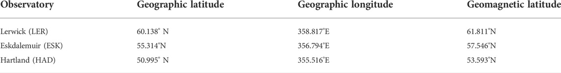
TABLE 1. Observatory locations with geomagnetic coordinates in year 2020.0.

Ideally, we wish to be able to predict the ground variations of the magnetic field to a suitable accuracy in order to compute the ground electric field and subsequently GIC flow in grounded infrastructure. This would provide timely forewarning and actionable information, for example to civil authorities and industrial operators in the event of a severe space weather event. This work is the first to attempt to produce a direct estimate of geomagnetic field variation at United Kingdom observatories using a RNN as opposed to other regression methods (e.g., [16]).

In Section 2, we describe the data selection and preprocessing as well as the construction of the machine learning models. In Section 3 we show the result of forecasting the 7–9th September 2017 storm using simple correlation analysis. We discuss the overall performance of the models in Section 4, where we also suggest further improvements to the forecasting methods.

2 Data and methods

2.1 Ground Magnetic and solar wind data

We use the interplanetary magnetic field (IMF) and solar wind plasma data as measured at the L1 Lagrange point to predict |B_H| and $\left|\frac{\mathrm{d}{B}_H}{\mathrm{d}t}\right|$ at the three United Kingdom observatories, ESK, HAD and LER. These observatories are chosen as they represent a range of latitudes within the British Isles. The geographic and geomagnetic coordinates are given in Table 1. The following data are used, chosen based on correlation to |B_H| and $\left|\frac{\mathrm{d}{B}_H}{\mathrm{d}t}\right|$: IMF B_Y and B_Z in the geocentric solar magnetospheric (GSM) reference frame; solar wind velocity v; and solar wind proton density n. For training and validation, these data were extracted from the OMNI dataset [17], which was accessed through the Heliophysics Application Programming Interface (HAPI)¹. For model testing, real time satellite measurements from the L1 Lagrange point were used to evaluate the models’ efficiency.

To train and test the NNs, minute-mean cadence magnetometer measurements were gathered through the ESA Swarm data access service VirES² using the Python package Viresclient³, with the core magnetic field removed using CHAOS-7 [18] leaving the residual field which is a combination of the crustal and external fields. We then compute and subtract the long term average of the residuals at each observatory to remove the constant crustal field bias in each component. From the northward, B_N, and eastward, B_E, magnetic field components, we calculate the magnitude of the horizontal field component, |B_H| and its time derivative from:

$|B_H|=\sqrt{B_N^2+B_E^2};\left|\frac{\mathrm{d}{B}_H}{\mathrm{d}t}\right|=\sqrt{{\left(\frac{\mathrm{d}{B}_N}{\mathrm{d}t}\right)}^2+{\left(\frac{\mathrm{d}{B}_E}{\mathrm{d}t}\right)}^2}(1)$

Here, we discretise the time derivative by computing the backwards difference between two timesteps of Δt = 1 min.

2.2 Machine learning models

Deep learning models created in this study were constructed using the TensorFlow Keras environment [19]. Each model takes the four IMF and solar wind plasma parameters as well as |B_H| or $\left|\frac{\mathrm{d}{B}_H}{\mathrm{d}t}\right|$ prior to that instant as input. For any given time t, the model ingests the six parameters at timesteps (t − j) to t where j ∈ [0, T] and T is the length of the input window. The models then predict |B_H(t + i)| or $\left|\frac{\mathrm{d}{B}_H}{\mathrm{d}t}(t+i)\right|$ where i is the forecasting lead time. The right set of hyperparameters is crucial for model performance, and the optimal hyperparameter configuration may vary with forecast parameter, lead time and observatory. All individual models have been hyperparameter-tuned using the 5-fold grid search cross validation algorithm by scikit-learn [20].

2.2.1 Long short-term memory network

The LSTM network is a type of RNN whose performance is particularly well suited for time series forecasting [21]. Unlike most RNNs, which are connected between consecutive timesteps, the LSTM network has an additional cell state which acts as a long-term memory and is thus able to store information in each memory cell from multiple timesteps [12,15]. The LSTM network takes a 3-dimensional input vector with variables (samples, timesteps, parameters). In this study, we have chosen a time window length of T = 30 min. The general LSTM model setup has either one or two hidden LSTM layers feeding to an output dense (fully connected) node. Each LSTM model is cross-validated for the number of LSTM layers (1 or 2), LSTM cells in each layer (4, 16 or 32) and the activation function in the LSTM layers (sigmoid or tanh). This gives 60 possible LSTM model configurations for forecasting each parameter (|B_H| or $\left|\frac{\mathrm{d}{B}_H}{\mathrm{d}t}\right|$) at each lead time (0, 5, 15 or 30 min). The best hyperparameter configuration for each forecasting model was determined using 5-fold grid search cross validation. Figure 1A shows an example of the model configuration and associated hyperparameters for the ${\left|\frac{\mathrm{d}{B}_H}{\mathrm{d}t}\right|}_{\text{max}30}$ LSTM forecast at LER (see Supplementary Tables S1–S4 for the hyperparameter configuration for each model).

FIGURE 1

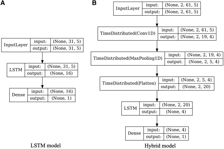
FIGURE 1. Keras model architecture for 30-min forecast of $\left|\frac{\mathrm{d}{B}_H}{\mathrm{d}t}\right|$ at LER. (A) shows LSTM architecture and (B) shows hybrid CNN-LSTM architecture. See Section 2.2 for details.

2.2.2 Hybrid CNN-LSTM networks

Unlike the LSTM network, which reads in the data in time-windows, CNNs have the ability to process an entire input matrix at once, making them very flexible. The key features of a CNN are the convolution kernels, which move across an input matrix and detect features in the data, and the pooling layer, which condenses the information from the convolution kernels. In 2-dimensional CNNs, the convolution and pooling kernels move along the input data in two dimensions, which has proven particularly successful for identifying features in image classification (e.g., [22]). For multivariate time series forecasting, where we are only interested in detecting temporal features, a useful CNN architecture is the 1-dimensional CNN (1D CNN). Here, the convolution kernels only move along one direction. For further details about CNNs in timeseries forecasting we refer to Siciliano et al. [15] for general CNN structures in space weather forecasting and Granat [23] for particular detail of 1D CNNs.

We developed a bespoke hybrid CNN-LSTM model that consists of a series of CNNs feeding into an LSTM layer before predicting an output. The general setup of the hybrid model is as follows: a CNN, consisting of a 1D-convolutional hidden layer, a 1D-MaxPooling layer and a Flatten layer, is wrapped in a TimeDistributed layer. This then feeds into an LSTM layer, where all LSTM cells are fully connected to an output node, which gives the prediction. For the hybrid model, the hyperparameter cross-validation was between the number of CNN filters (4, 8 or 12), the kernel size (5 or 7), the LSTM activation function (sigmoid or tanh) and the number of LSTM cells in the LSTM layer (1 or 4). The CNN kernel stride length is set to be half of the kernel size. The hybrid model takes a 4-dimensional input vector of variables (samples, subsequences, timesteps, parameters). The subsequences define how many windows are being loaded into the TimeDistributed CNN layer, and in turn, how many data are parsed to the LSTM layer, and the timesteps are the number of data within each subsequence. For each output, 2 h (T = 120) of input data are used. From testing different subsequence-timestep splits, the optimal split was found to be two subsequences of 60 timesteps, i.e., the CNN layers read in 60 timesteps and 2 CNN windows are then fed into the LSTM layer for each output. As with the LSTM model, the best hyperparameter configuration for each model was found using the 5-fold grid search cross validation. The model configuration for the hybrid model forecasting ${\left|\frac{\mathrm{d}{B}_H}{\mathrm{d}t}\right|}_{\text{max}30}$ at LER is shown in Figure 1B.

2.3 Data selection

As with most damaging geohazards (e.g., earthquakes, landslides, volcanoes), very large events in our case geomagnetic storms - are relatively rare occurrences [24]. This presents the main problem for training a machine learning model: the lack of data makes it difficult to develop reliable empirical relationships for forecasting extreme events, since they are likely to overfit on quiet periods when built on the entire dataset (e.g., [3,12,22]). In order to avoid over-training the models on geomagnetically quiet periods, we select storm events based on a certain exceedance threshold at each observatory within ±8 h of the threshold breach. For every timestamp $|\frac{\mathrm{d}{B}_H}{\mathrm{d}t}|$ that exceeds a certain value, the training and validation data are saved with an interval of 8 h before and after the time of exceedance. After inspection and experimentation, the exceedance value was set to be 25 nT min⁻¹ for LER and ESK, and 20 nT min⁻¹ for HAD. These thresholds all exceed the 99.95% percentiles for each observatory. The models are trained on event data (large storms) from 1997 to 2012, and validated with storms from 2012 to 2016. The number of training and validation event days for each observatory are given in Table 2.

TABLE 2

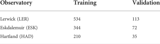
TABLE 2. Number of event days included in the training and validation sets for each observatory.

2.4 Data preprocessing

Wintoft et al. [1] showed that it is difficult to predict any variations in |B_H| or $|\frac{\mathrm{d}{B}_H}{\mathrm{d}t}|$ at minute resolution. Instead we filter the magnetic field data using a rolling maximum filter, as shown in Figure 2. We set the rolling maximum filter window size equal to the forecasting lead time. The steps for computing the 30 min $\left|\frac{\mathrm{d}{B}_H}{\mathrm{d}t}\right|$ and, ${\left|\frac{\mathrm{d}{B}_H}{\mathrm{d}t}\right|}_{\text{max}30}$ forecast are as follows. Firstly, we filter the measured solar wind and magnetic data, as shown in Figure 2A, using a backwards rolling maximum window (Figure 2B, solid blue line). The backward rolling maximum will set the value at each timestep as the maximum value observed within the previous 30 min. Next, the filtered data are fed into the model, with the desired output being the maximum value in the next 30 min, as shown by the solid red line in Figure 2C. This is the same as applying a 30 min forwards rolling maximum filter to the raw data, as the forward rolling maximum will set the value at each timestep to the maximum value to be observed in the next 30 min. The solid red line in Figure 2C thus shows the ideal 30 min forecast. The NN models are therefore trained to predict the forward maximum within the interval given by the lead time, rather than the minute cadence changes.

FIGURE 2

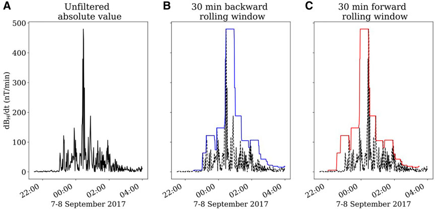
FIGURE 2. Example of rolling maximum window for $|\frac{\mathrm{d}{B}_H}{\mathrm{d}t}{|}_{30}$ during the 7th to 8th September 2017 at LER. (A) shows the unfiltered |dB_H/dt|. (B) shows the 30 minute backwards rolling window and (C) shows the 30 minutes forward rolling window.

After picking events and applying the rolling maximum filter to the data, the full time series for each input parameter is normalised to its feature range such that the values lie between 0 and 1 in order to optimise learning. This normalisation for each datum x in the time series for each parameter is given by:

$x_{\mathit{scaled}}=\frac{x-x_{\mathit{min}}}{x_{\mathit{max}}-x_{\mathit{min}}}(2)$

The full dataset is then split into training and validation parts and fed into the models. Each model uses the adaptive moment estimation (Adam) for optimisation and mean squared error (MSE) as a cost function:

$\text{MSE}=\frac{1}{N}\sum _{i=1}^N{\left({\widehat{y}}_i-y_i\right)}^2(3)$

Here, N is the number of samples in the event, y is the observed value and $\widehat{y}$ is the predicted value. We chose MSE as it penalises larger errors more harshly than most functions, though other performance criteria are also available, as outlined in Camporeale [22].

3 Results

We developed 24 models, one for each of the three observatories, trained to forecast either |B_H| or ${\left|\frac{\mathrm{d}{B}_H}{\mathrm{d}t}\right|}_{\text{max}i}$ with i = 0 (nowcasting), 5, 15 or 30 min lead times. Each model was then evaluated using data from the 7–9th September 2017 storm [25]. This storm was chosen as it was reasonably large (Kp 8+) and had a measurable effect on the ground magnetic field at all three observatories. Werner et al. [26] describe the storm as resulting from multiple coronal mass ejection interactions and provide a chronological overview of the events. It is outside the training and validation date range and so is an independent test of the forecasting capability.

Figure 3 shows the DSCOVR and ground observatory data as well as the 30 min forecasts for the 7–9th September 2017 storm, with the ground response to the first magnetospheric disturbance shown in the insets to the ground observatory data panels. At all three observatories, a peak in |B_H| and $\left|\frac{\mathrm{d}{B}_H}{\mathrm{d}t}\right|$ occurred at 23:00 as a response to the first part of the storm and was followed by stronger substorm activity 1.5 h later. The amplitude of the peak increases with observatory latitude (Figure 3). For the 30 min forecasts at LER (Figures 3D,E, the models appear to predict the changes in |B_H| and $|\frac{\mathrm{d}{B}_H}{\mathrm{d}t}|$ for the onset of the storm, with increases shown in both model forecasts 30 min before they occur in the observations. However, about an hour after the storm initiation, the forecasting power diminishes though the predictions still follow the maximum values in |B_H| and $|\frac{\mathrm{d}{B}_H}{\mathrm{d}t}|$ but at shorter lead times than 30 min.

FIGURE 3

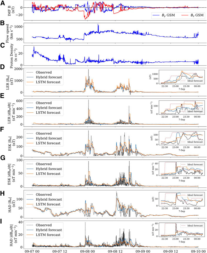
FIGURE 3. DSCOVR measurements and ground observatory measurements, and predictions for the 7th-9th September 2017 storm. Solar wind (A) IMF B_Y and B_Z components, (B) the solar wind speed velocity and (C) density. Measured (black) and 30-min forecast (blue for hybrid, orange for LSTM) horizontal magnetic field and its time derivative at (D,E) LER, (F,G) ESK and (H,I) HAD observatory. The inset figures show observed B_H and $\frac{\mathrm{d}{B}_H}{\mathrm{d}t}$ and forecast |B_H|_{max 30} and ${\left|\frac{\mathrm{d}{B}_H}{\mathrm{d}t}\right|}_{\text{max}30}$ during the storm onset around midnight on 7th September 2017. Ideal forecasts are shown in red.

Considering this reduction in forecast power after the initial phase, we split the storm into two parts: the initial part of the storm where the ground magnetic field is directly driven by the solar winds, and the later phase which was indirectly driven by substorm and auroral electrojet enhancement. We consider the directly driven part of the storm to last for 45 min after the storm commencement. To evaluate ability to forecast only this part of the storm, we ignore data from 45 min after the storm commencement until |B_H| and $|\frac{\mathrm{d}{B}_H}{\mathrm{d}t}|$ reduce to near zero levels.

Figure 4 shows the correlation between the forecasted and observed |B_H|_{max 30} and ${\left|\frac{\mathrm{d}{B}_H}{\mathrm{d}t}\right|}_{\text{max}30}$ at each of the observatories for the 7–9th September 2017 storm. The best fit line for each forecasting model has been found using the method of least squares, and is shown as a dotted line for the full storm and solid line for the directly driven part. The gradient and intercept for the best fit lines are given in Table 3. We note that these best-fit lines have a non-zero intercept, suggesting the presence of a general systematic bias in model prediction. Figure 4 shows that forecasts at LER perform better for the full storm, with a higher correlation, as compared to the other observatory forecasts using either the LSTM or hybrid model. We also observe that the |B_H|_{max 30} forecasts show a better correlation than the ${\left|\frac{\mathrm{d}{B}_H}{\mathrm{d}t}\right|}_{\text{max}30}$ forecasts. This suggests the variability in $\frac{\mathrm{d}{B}_H}{\mathrm{d}t}$ is too complicated for the machine learning models to replicate as other non-linear or indirect processes are involved [27].

FIGURE 4

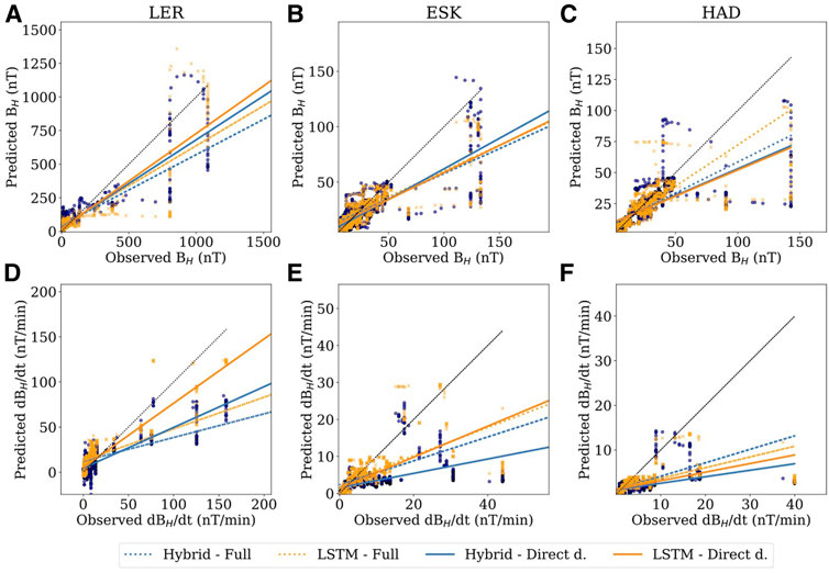
FIGURE 4. Correlation plots for forecasts of |B_H| (A–C) and |dB_H/dt| (D–F) with 30 min lead time at LER (A,D), ESK (B,E), and HAD (C,F). Orange represents LSTM and blue hybrid models; solid lines are for directly driven parts of the storm and dotted lines represent full storm. Gradient and intercept for best fit line are given in Table 3. Dotted black line shows the 1:1 line for reference.

TABLE 3

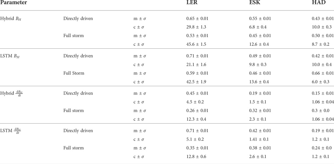
TABLE 3. Gradient, m, and intercept, c, for best fit lines of form y = mx + c for 30 min forecast shown in Figure 4. σ is the standard deviation of the best fit gradient and intercept parameters derived from the covariance matrix of the least squares fit.

When comparing the relative performance between the hybrid and LSTM models, we see that the LSTM forecast generally has a higher correlation. This may relate to the LSTM models’ ability to capture the “blockiness” of the rolling maximum filter, leading to less variability at the higher cadences. The models inability to capture this “blockiness” appears as vertical features in the scatter plots. This is particularly obvious in the |B_H|_{max 30} forecast in Figure 4 for LER at observed values around 1,000 nT or ESK at observed values around 130 nT.

Comparing the best fit line for the full storm to the directly driven part, we see that there is only a small change for both |B_H|_{max 30} forecasts at LER and hybrid ${\left|\frac{\mathrm{d}{B}_H}{\mathrm{d}t}\right|}_{\text{max}30}$ at ESK, suggesting that there is no significant difference in performance for the directly and indirectly driven parts of the storm for these components. However, we see a significant increase in correlation for the ${\left|\frac{\mathrm{d}{B}_H}{\mathrm{d}t}\right|}_{\text{max}30}$ forecast at LER and moderate increase for the hybrid |B_H|_{max 30} at ESK when the indirectly driven parts of the storm are excluded. This suggests that the LER and hybrid |B_H|_{max 30} ESK forecast models perform better during the directly driven parts of the storm. Furthermore, the best fit lines for all models show a smaller intercept value for the directly driven parts of the storm, when compared to the full storm, implying better performance during the directly driven part. We thus propose that the LER and ESK models perform better during the directly driven parts of the storm as compared to the full storm. Considering the HAD forecasts, the best fit line has a much shallower gradient for the directly driven parts of the storm than for the full storm with the HAD forecasts performing poorly in general.

Figure 5 shows the correlation between the observed and predicted |B_H|_{max i} and ${\left|\frac{\mathrm{d}{B}_H}{\mathrm{d}t}\right|}_{\text{max}i}$ at LER for i = 0 (nowcast), 5, 15, and 30 min lead time using the hybrid (blue) and LSTM (orange) models. Similar figures for the ESK and HAD forecasts are found in the Supplementary Material. The gradient and intercept of the best fit lines are given in Table 4. The LSTM nowcasts all show a best fit gradient very close to 1. This suggests that the LSTM model is capable of reproducing the changes in |B_H| and $|\frac{\mathrm{d}{B}_H}{\mathrm{d}t}|$ from the input solar wind parameters. The |B_H| hybrid nowcast also shows a good linear fit, but has a larger scatter, implying that the hybrid models are less able to reproduce the observed magnetic field from the input data; the difference is even more marked for $|\frac{\mathrm{d}{B}_H}{\mathrm{d}t}|$.

FIGURE 5

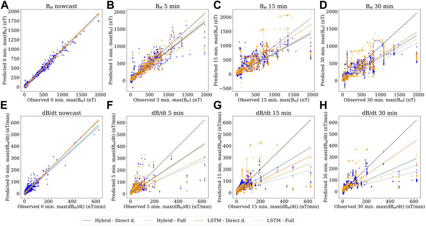
FIGURE 5. Correlation plots for now- and forecasts of |B_H| (A–D) and |dB_H/dt| (E–H) at 5, 15 and 30 min lead time at LER. Orange represents LSTM and blue hybrid models; solid lines are for directly driven parts of the storm and dotted lines represent full storm. Gradient and intercept for best fit line are given in Table 4. Dotted black line shows the 1:1 line for reference.

TABLE 4

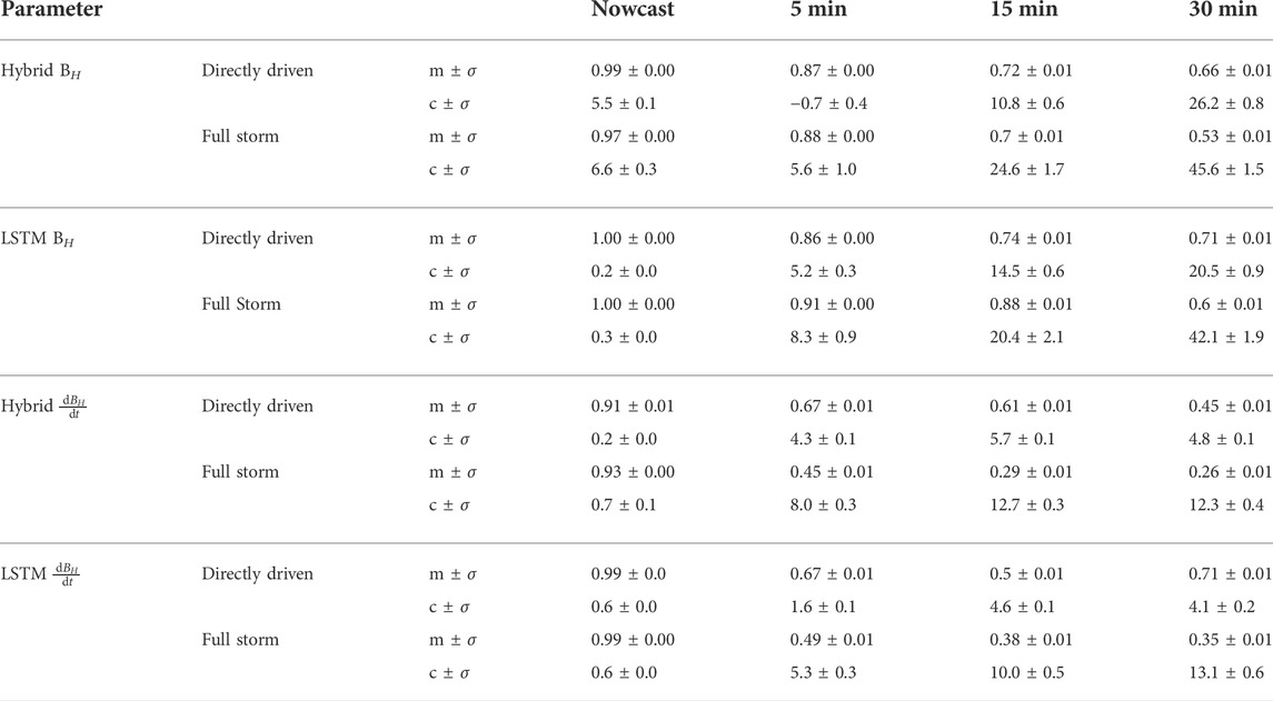
TABLE 4. Gradient, m, and intercepts, c, for best fit lines for now- and forecasts at LER as shown in Figure 5. σ is the standard deviation of the best fit gradient and intercept parameters derived from the covariance matrix of the least squares fit.

With increasing lead time, the correlation between observed and forecast values decreases. This is clearer in the ${\left|\frac{\mathrm{d}{B}_H}{\mathrm{d}t}\right|}_{\text{max}i}$ than the |B_H|_{max i} forecasts (with the exception of the LSTM 15 min $|\frac{\mathrm{d}{B}_H}{\mathrm{d}t}|$ forecast). Despite the decrease, we still observe gradients above 0.6 for all |B_H|_{max i} forecasts at LER, and we thus consider the models to have some forecasting power.

For completeness, the square-root of the MSE (RMSE) values for each model forecasting the test storm are shown graphically in Figure 6 for all three observatories and given in Supplementary Table S5. These show similar trends to that observed from the correlation analysis in Table 4, Supplementary Table S6, S7. A general increase in RMSE is observed with increasing lead time. In the nowcasts for all three observatories, the LSTM significantly outperforms the hybrid model, but for larger lead times, their RMSEs are comparable. The only exception to this is the models forecasting |B_H| with a 30 min lead time at HAD, where the LSTM performs consistently better in forecasting the full storm. We also see a significant difference in RMSE between forecasting the full storm as opposed to forecasting the directly driven parts only, which is again consistenct with the observations from the correlation analysis.

FIGURE 6

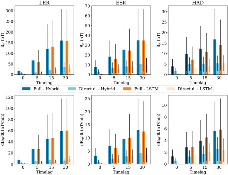
FIGURE 6. RMSE for each model forecasting the test storm at each Timelag in minutes LER, ESK and HAD. Blue colours represent the hybrid model, orange colours represent the LSTM model. Error bars signify one standard deviation in the RMSE. Note the difference in y-scale in each plot.

To investigate further the forecasting power of the models during the directly driven part of the storm compared to the full storm, we plot in Figure 7 the correlation coefficient, R, between the data and the forecast for various time shifts at LER. (Similar figures for the ESK and HAD forecasts are found in the Supplementary Material.) If the forecasts were perfect, there would be a sharp peak at 0 timeshift (i.e., no lag), and if the forecast consistently predicted 5 min behind the data, the peak would be at −5. The dashed lines show the correlation for the full test storm forecasts, and the peaks are observed at a lag equivalent to the negative of the forecast lead time. This suggests that the overall forecasting power is reduced when considering the full storm, and that the models could be considered inefficient nowcasts rather than forecasts.

FIGURE 7

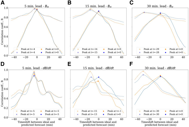
FIGURE 7. Temporal correlation between ideal and model-generated forecast of |B_H| (A–C) and |dB_H/dt| (D–F) at LER. × and • marks the peak correlation. As before, orange represents LSTM and blue hybrid models; solid lines are for directly driven parts of the storm and dotted lines represent full storm.

By considering only the directly driven parts of the storms, we see significant change in forecasting power for some of the models. The solid lines in Figure 7 show a shift in the peak for all three |B_H| forecasts at LER, as well as in the ${\left|\frac{\mathrm{d}{B}_H}{\mathrm{d}t}\right|}_{\text{max}30}$ forecast, which all show a peak at zero lag. There is a slight decrease in correlation for all of these models, compared to their full-storm equivalents, but they still show better performance than with the full storm data at 0 timelag. For the ${\left|\frac{\mathrm{d}{B}_H}{\mathrm{d}t}\right|}_{\text{max}15}$ forecast, the hybrid model manages to sustain a clear forecasting capability in the directly driven parts of the storm, but the LSTM model performs significantly worse during this period. From this shift in peak correlation, we conclude that the |B_H| models as well as the hybrid ${\left|\frac{\mathrm{d}{B}_H}{\mathrm{d}t}\right|}_{\text{max}15}$ and both ${\left|\frac{\mathrm{d}{B}_H}{\mathrm{d}t}\right|}_{\text{max}30}$ models perform better during the directly driven parts of the storm.

4 Discussion

We present a new study examining the use of convolutional and recurrent neural networks to predict ground level geomagnetic field variation at three mid-latitude observatories in the United Kingdom. Clearly the relationship is complex and non-linear in detail. This work provides evidence that some predictive power appears in the connection between the L1 solar wind and magnetic field variation on Earth.

4.1 Evaluating the models

The statistical results from evaluating the forecasts at LER for 5, 15 and 30 min lead times are promising. Though the models generally performed poorly when attempting to predict variation during the entire storm, a significant increase in model performance was observed in most cases for the directly driven parts of the storm. |B_H| forecasts at all three lead times showed a clear peak at 0 min in the temporal correlation plots. This result is also observed for forecasting $\left|\frac{\mathrm{d}{B}_H}{\mathrm{d}t}\right|$ at 15 and 30 min at LER, but only using the hybrid model for a 15 min lead time. We therefore conclude that the models have forecasting power for the directly driven parts of the storm at LER.

Looking at the results from the other observatories (see Supplementary Figure S1–S4; Supplementary Table S6, S7), the ESK |B_H| forecasts show poor temporal correlation when forecasting the full storm, but the correlation has a clear peak at zero for the 15 and 30 min forecasts for the directly driven parts of the storm, though with a decrease in magnitude. When considering only the directly driven parts of the storm at ESK, we see a significant decrease in linear fit for the LSTM model, but an increase for the hybrid model. From these observations, we conclude that the ESK |B_H| forecasts are not as good as those for LER, but again the models do have some forecasting capability. The $\left|\frac{\mathrm{d}{B}_H}{\mathrm{d}t}\right|$ forecasts at ESK are less successful as the temporal correlation peaks at the negative of the lead time for both the full and the directly driven parts of the storm. Neither of the |B_H| or the $\left|\frac{\mathrm{d}{B}_H}{\mathrm{d}t}\right|$ models for HAD showed any useful forecasting power.

Overall, this suggests that RNNs are useful tools in forecasting geomagnetic storm onsets at mid-to high latitudes. Keesee et al. [4] investigated this by forecasting B_E and B_N separately, in order to predict |B_H| and $\left|\frac{\mathrm{d}{B}_H}{\mathrm{d}t}\right|$, comparing LSTM performance to that of a simple feed-forward NN. They found that their LSTM models were comparable to random predictions. However, in contrast to us, they did not utilise the memory-aspect of the LSTM algorithm. Our models differ from theirs by including information about either |B_H| or $\left|\frac{\mathrm{d}{B}_H}{\mathrm{d}t}\right|$ from up to 2 h prior to the forecast, which results in a clear ability to predict the directly driven parts of the storm. Quantitative comparisons are not straightforward, however, as they use a classification-based evaluation method.

4.2 Applications with real time data

As mentioned in Section 2.1, the models were trained and validated using data from the OMNI scientific dataset, but were tested using real-time DSCOVR data. We note that there is a temporal difference between the OMNI data and the real-time data from the L1 Lagrange point, since the OMNI data have been time-shifted to Earth’s bow shock [28]. The OMNI dataset was chosen for its easy access and the relative lack of data gaps compared to the real-time stream. Most data gaps in the training and validation data were shorter than the forecasting lead times, and were thus negligible when the rolling max filter was applied.

We further note, similar to Smith et al. [29], that using the OMNI dataset to create models with the ability to capture impulsive phenomena, such as sudden commencements, is not ideal. By comparing model performance on the test storm using data from DSCOVR and OMNI, we found that the models tested on OMNI data were incapable of capturing such impulsive phenomena. However, we attribute our models’ ability to forecast using real-time data, regardless of being trained on OMNI data, to the stripping of temporal information in our preprocessing pipeline (particularly the rolling max-filter). We interpret the training process such that the models associate sharp peaks in the IMF input with sharp peaks in the ground magnetic measurements. Thus, using real-time L1 Lagrange point measurements allows the models to infer an increase in |B_H| or $|\frac{\mathrm{d}{B}_H}{\mathrm{d}t}|$ before a solar storm reaches Earth, assuming it is reasonably continuous and complete [30].

4.3 Forecasting extreme values

The nowcast models tend to under-predict extreme values. This relates to the process of normalisation of the input data for machine learning algorithms. As noted by Siciliano et al. [15], normalisation compresses the data into a smaller range such that, if the predicted extreme values were too low, the resulting value after converting to the full scale would be diminished. They proposed standardising the data to the mean before input, but this has its own issues, as it assumes the data to be approximately normally distributed. Thomson et al. [24] show that geomagnetic variations driven by space weather are better modelled as a generalised extreme value distribution. Hence, extreme values would be incorrectly represented if normalised to centre about a particular mean. Therefore, a better way to preprocess the data for machine learning training and prediction may be to normalise using a Pareto distribution, or other extreme value statistic, fitted to the data from each observatory to be modelled.

An alternative approach would be to evaluate the models’ ability to predict exceedance of extreme thresholds within a given time window, rather than their ability to predict observed values at minute resolution, thus changing the problem from a regression to a classification problem. Classification methods, such as the binary event analysis proposed by Pulkkinen et al. [31] and later refined by Welling et al. [32], allow for easier comparison of observatories at different latitudes, as the associated error will not be purely magnitude-dependent in contrast to the MSE. However, this method involves further complexity, as it requires defining representative thresholds for each observatory.

4.4 How much of the past is required to predict the future?

We have assumed that each forecast and nowcast model performed best with the same temporal input length. The 30 min input length for the LSTM models was chosen because it should encompass the IMF variations observed at DSCOVR before ground magnetic field effects are observed, and the 60 × 2 sequences for the hybrid models were chosen for the CNN layer to have more data to filter. When analysing optimal IMF and solar plasma input parameters for Kp prediction, Tan et al. [12] performed a correlation analysis for their input parameters at increasing timelags against Kp to determine at what timestep the information became obsolete; they found a 6 h input series with a cadence of 1 h to be optimal. A similar approach to determine the optimal input timesteps from correlating with |B_H|_{max i} or ${\left|\frac{\mathrm{d}{B}_H}{\mathrm{d}t}\right|}_{\text{max}i}$ for each lead time i is a clear suggestion for future work. Alternatively, the optimal choice of input timesteps (and subsequences for the hybrid model), could be included in the grid search cross validation. We note that Tan et al. [12] used 3 parameters for forecasting Kp, all of which are composite indicies, but an initial analysis we carried out indicated the four solar wind parameters chosen were sufficient for this study.

4.5 Model performance related to observatory latitude

We found a significant difference in the number of events at each observatory, as shown in Table 2. Lerwick has almost twice as many hours of geomagnetic event data and the size of these events is significantly larger (see Figure 3). This is expected as observatories at higher latitudes experience larger effects from the influence of the auroral electrojet [33,34]. During the data processing this was not fully appreciated when picking events from the full datasets at each observatory as the $\left|\frac{\mathrm{d}{B}_H}{\mathrm{d}t}\right|$ threshold is almost equal for all observatories. This imbalance in the number of samples across datasets could be avoided by binning observatories at similar geomagnetic latitudes (e.g., [16]). In this way, models could be trained for latitude sectors rather than for individual observatories, and would allow for a more comprehensive training and validation dataset. However, local induction effects are different at each observatory, which would also have to be considered.

4.6 LSTM vs. hybrid networks

We have determined that there is a difference in performance between the LSTM and hybrid CNN-LSTM networks. Considering first the nowcasts, the LSTM model showed a best fit line with a gradient close to 1 for both |B_H| and $\left|\frac{\mathrm{d}{B}_H}{\mathrm{d}t}\right|$, replicating the entire data profile, apart from the extreme values. Conversely, the hybrid models showed a larger scatter around the best fit line, only catching the major changes in |B_H| and under-predicting $\left|\frac{\mathrm{d}{B}_H}{\mathrm{d}t}\right|$. The LSTM model is therefore better at replicating the changes in the ground magnetic field in real time.

For the forecasts, the hybrid models tend to perform worse than the LSTM in most cases, the exceptions being the ${\left|\frac{\mathrm{d}{B}_H}{\mathrm{d}t}\right|}_{\text{max}15}$ forecasts at LER and ESK. This may be because the LSTM model is generally better at reproducing the rolling window-like constant values over longer time periods, whereas the hybrid model predictions fluctuate more. The reason why the LSTM models perform poorly at 15 min remains unknown, but may originate in the backward rolling window in the input data and the backward rolling window prediction goal just overlapping, since the travel time for fast solar wind from the L1 point to the Earth is of the order of 30 min.

Therefore, although the hybrid models perform comparably at most observatories, and outperfom LSTM in the ${\left|\frac{\mathrm{d}{B}_H}{\mathrm{d}t}\right|}_{\text{max}15}$ forecasts, we conclude that the LSTM network is the better model for forecasting directly driven ground changes in the magnetic field. Evaluating the performance of three models-LSTM, hybrid CNN-LSTM and a pure 1D CNN-in order to determine whether the hybrid model performs worse and why is an obvious line of enquiry. If both the CNN and LSTM models perform better than the hybrid model, it might be that the hybrid model requires a smoother connection between the CNN and LSTM layers for example.

5 Conclusion

Horizontal geomagnetic field data gathered from three United Kingdom observatories, Lerwick, Eskdalemuir and Hartland, were correlated with IMF and solar plasma data from the L1 Lagrange point. Two machine learning approaches were adopted for each observatory: a pure LSTM network and a hybrid CNN-LSTM model. Each architecture was used to develop the following models: one for nowcasting the horizontal geomagnetic field and its time derivative, and one for forecasting with a lead time of 5, 15 and 30 min. The optimal hyperparameters for each model were trained using large geomagnetic storms between 1997 and 2016, and the models were tested on the 7–9 September 2017 storm. Overall, the pure LSTM networks were found to outperform the hybrid models, with the exception being the 15 min $\left|\frac{\mathrm{d}{B}_H}{\mathrm{d}t}\right|$ forecasts at Lerwick and Eskdalemuir.

The forecast models were only able to predict the directly driven parts of geomagnetic storms in the first few hours before magnetic reconnection (substorms) become the dominant driver. The models were better at forecasting at higher geomagnetic latitudes, where the ground response to magnetospheric disturbances is more enhanced.

Further improvements include expanding the input parameters to include the magnetic local time and bin multiple observatories at similar latitudes together to expand the training datasets. Overall, we suggest that machine learning algorithms perform best when there are strong physical links between the driving parameters and the ground effects.

Data availability statement

Publicly available datasets were analyzed in this study. These data can be found here: https://cdaweb.gsfc.nasa.gov/registry/hdp/hapi https://vires.services/.

Author contributions

FDM collected data, wrote the code, and analysed the results. CDB and KAW designed the project and analysed results. All three contributed equally to the writing of the manuscript.

Funding

This work is funded under United Kingdom Natural Environment Research Council Grant NE/P017231/1 and NE/P017290/1 “Space Weather Impact on Ground-based Systems (SWIGS).” This work has also received funding from the European Union’s Horizon 2020 research and innovation program under grant agreement No 870405 (EUHFORIA 2.0). Open access funding was provided by the University of Edinburgh under agreement with UKRI.

Acknowledgments

We wish to acknowledge assistance from Ashley Smith for help with coding and advice on data access. FDM acknowledges funding from a University of Edinburgh College Vacation Scholarship. We acknowledge use of NASA/GSFC’s Space Physics Data Facility’s OMNIWeb (or CDAWeb or ftp) service, and OMNI data. The results presented in this paper rely on data collected at magnetic observatories. We thank the national institutes that support them and INTERMAGNET for promoting high standards of magnetic observatory practice (www.intermagnet.org).

Conflict of interest

The authors declare that the research was conducted in the absence of any commercial or financial relationships that could be construed as a potential conflict of interest.

Publisher’s note

All claims expressed in this article are solely those of the authors and do not necessarily represent those of their affiliated organizations, or those of the publisher, the editors and the reviewers. Any product that may be evaluated in this article, or claim that may be made by its manufacturer, is not guaranteed or endorsed by the publisher.

Supplementary material

The Supplementary Material for this article can be found online at: https://www.frontiersin.org/articles/10.3389/fphy.2022.1017781/full#supplementary-material

Footnotes

¹https://cdaweb.gsfc.nasa.gov/registry/hdp/hapi, last accessed 01-Jul-2022.

²https://vires.services/, last accessed 01-Jul-2022.

³doi.org/10.5281/zenodo.4694720

References

1. Wintoft P, Wik M, Viljanen A. Solar wind driven empirical forecast models of the time derivative of the ground magnetic field. J Space Weather Space Clim (2015) 5:A7. doi:10.1051/swsc/2015008

CrossRef Full Text | Google Scholar

2. Viljanen A, Wintoft P, Wik M. Regional estimation of geomagnetically induced currents based on the local magnetic or electric field. J Space Weather Space Clim (2015) 5:A24. doi:10.1051/swsc/2015022

CrossRef Full Text | Google Scholar

3. Bailey RL, Leonhardt R, Möstl C. Forecasting local GICs from solar wind data [Quick View session]. European: European Space Weather Symposium (2020).

Google Scholar

4. Keesee AM, Pinto V, Coughlan M, Lennox C, Mahmud MS, Connor HK. Comparison of deep learning techniques to model connections between solar wind and ground magnetic perturbations. Front Astron Space Sci (2020) 7:72. doi:10.3389/fspas.2020.550874

CrossRef Full Text | Google Scholar

5. Hapgood M. Space weather. Oklahoma: IOP Publishing (2017). p. 2399–891.

Google Scholar

6. Pulkkinen A, Bernabeu E, Thomson A, Viljanen A, Pirjola R, Boteler D, et al. Geomagnetically induced currents: Science, engineering, and applications readiness. Space Weather (2017) 15(7):828–56. doi:10.1002/2016sw001501

CrossRef Full Text | Google Scholar

7. Campanyá J, Gallagher PT, Blake SP, Gibbs M, Jackson D, Beggan CD, et al. Modeling geoelectric fields in Ireland and the UK for space weather applications. Space Weather (2019) 17(2):216–37. doi:10.1029/2018sw001999

CrossRef Full Text | Google Scholar

8. Hapgood M, Angling MJ, Attrill G, Bisi M, Cannon PS, Dyer C, et al. Development of space weather reasonable worst case scenarios for the UK national risk assessment. Maryland: Space Weather (2021).

Google Scholar

9. Oughton EJ, Hapgood M, Richardson GS, Beggan CD, Thomson AWP, Gibbs M. A risk assessment framework for the socioeconomic impacts of electricity transmission infrastructure failure due to space weather: An application to the United Kingdom. Risk Anal (2018) 38(12):1022–43. doi:10.1111/risa.13229

CrossRef Full Text | Google Scholar

10. Wintoft P, Wik M, Matzka J, Shprits Y. Forecasting Kp from solar wind data: Input parameter study using 3-hour averages and 3-hour range values. J Space Weather Space Clim (2017) 7:A29. doi:10.1051/swsc/2017027

CrossRef Full Text | Google Scholar

11. Wintoft P, Wik M. Evaluation of Kp and Dst predictions using ACE and DSCOVR solar wind data. Space Weather (2018) 16(12):1972–83. doi:10.1029/2018sw001994

CrossRef Full Text | Google Scholar

12. Tan Y, Hu Q, Wang Z, Zhong Q. Geomagnetic index Kp forecasting with LSTM. Space Weather (2018) 16(4):406–16. doi:10.1002/2017sw001764

CrossRef Full Text | Google Scholar

13. Chakraborty S, Morley SK. Probabilistic prediction of geomagnetic storms and the K_p index. J Space Weather Space Clim (2020) 10:36. doi:10.1051/swsc/2020037

CrossRef Full Text | Google Scholar

14. Gruet MA, Chandorkar M, Sicard A, Camporeale E. Multiple-hour-ahead forecast of the Dst index using a combination of Long Short-Term Memory neural network and Gaussian process. Space Weather (2018) 16(11):1882–96. doi:10.1029/2018sw001898

CrossRef Full Text | Google Scholar

15. Siciliano F, Consolini G, Tozzi R, Gentili M, Giannattasio F, De Michelis P. Forecasting sym-H index: A comparison between long short-term memory and convolutional neural networks. Space Weather (2020) 18:e2020SW002589. Accepted Author Manuscript. doi:10.1029/2020SW002589

CrossRef Full Text | Google Scholar

16. Shore RM, Freeman MP, Coxon JC, Thomas EG, Gjerloev JW, Olsen N. Spatial variation in the responses of the surface external and induced magnetic field to the solar wind. JGR Space Phys (2019) 124(7):6195–211. doi:10.1029/2019ja026543

CrossRef Full Text | Google Scholar

17. King JH, Papitashvili NE. Solar wind spatial scales in and comparisons of hourly Wind and ACE plasma and magnetic field data. J Geophys Res (2005) 110(A2):A02104. doi:10.1029/2004ja010649

CrossRef Full Text | Google Scholar

18. Finlay CC, Kloss C, Olsen N, Hammer MD, Tøffner-Clausen L, Grayver A, et al. The CHAOS-7 geomagnetic field model and observed changes in the South Atlantic anomaly. Earth Planets Space (2020) 72(1):156. doi:10.1186/s40623-020-01252-9

PubMed Abstract | CrossRef Full Text | Google Scholar

19. François C, et al. Keras (2015). Available at: https://keras.io.

Google Scholar

20. Pedregosa F, Varoquaux G, Gramfort A, Michel V, Thirion B, Grisel O, et al. Scikit-learn: Machine learning in python. J Machine Learn Res (2011) 12(85):2825–30.

Google Scholar

21. Hochreiter S, Schmidhuber J. Long short-term memory. Neural Comput (1997) 9(8):1735–80. doi:10.1162/neco.1997.9.8.1735

PubMed Abstract | CrossRef Full Text | Google Scholar

22. Camporeale E. The challenge of machine learning in space weather: Nowcasting and forecasting. Space Weather (2019) 17(8):1166–207.

CrossRef Full Text | Google Scholar

23. Granat M. How to use convolutional neural networks for time series classification (2019). Retrieved from https://towardsdatascience.com/how-to-use-convolutional-neural-networks-for-time-series-classification-56b1b0a07a57 (Accessed Mar 25, 2021).

Google Scholar

24. Thomson AWP, Dawson EB, Reay SJ. Quantifying extreme behavior in geomagnetic activity. Space Weather (2011) 9(10). doi:10.1029/2011sw000696

CrossRef Full Text | Google Scholar

25. Dimmock AP, Rosenqvist L, Hall J-O, Viljanen A, Yordanova E, Honkonen I, et al. The GIC and geomagnetic response over Fennoscandia to the 7–8 September 2017 geomagnetic storm. Space Weather (2019) 17(7):2018SW002132–1010. doi:10.1029/2018sw002132

CrossRef Full Text | Google Scholar

26. Werner ALE, Yordanova E, Dimmock AP, Temmer M. Modeling the multiple CME interaction event on 6–9 September 2017 with WSA-ENLIL+Cone. Space Weather (2019) 17(2):357–69. doi:10.1029/2018sw001993

CrossRef Full Text | Google Scholar

27. Freeman MP, Forsyth C, Rae IJ. The influence of substorms on extreme rates of change of the surface horizontal magnetic field in the United Kingdom. Space Weather (2019) 17(6):827–44. doi:10.1029/2018sw002148

CrossRef Full Text | Google Scholar

28. King J, Papitashvili N. Spdf - OMNIweb service (2021). [Website]. Retrieved from https://omniweb.gsfc.nasa.gov/html/omni_min_data.html (Accessed March 28, 2021).

Google Scholar

29. Smith AW, Forsyth C, Rae IJ, Garton TM, Bloch T, Jackman CM, et al. Forecasting the probability of large rates of change of the geomagnetic field in the UK: Timescales, horizons, and thresholds. Space Weather (2021) 19(9). doi:10.1029/2021sw002788

CrossRef Full Text | Google Scholar

30. Smith AW, Forsyth C, Rae IJ, Garton TM, Jackman CM, Bakrania M, et al. On the considerations of using near real time data for space weather hazard forecasting. Space Weather (2022) 20(7):e2022SW003098. doi:10.1029/2022sw003098

CrossRef Full Text | Google Scholar

31. Pulkkinen A, Rastätter L, Kuznetsova M, Singer H, Balch C, Weimer D, et al. Community-wide validation of geospace model ground magnetic field perturbation predictions to support model transition to operations. Space Weather (2013) 11(6):369–85. doi:10.1002/swe.20056

CrossRef Full Text | Google Scholar

32. Welling DT, Ngwira CM, Opgenoorth H, Haiducek JD, Savani NP, Morley SK, et al. Recommendations for next-generation ground magnetic perturbation validation. Space Weather (2018) 16(12):1912–20. doi:10.1029/2018sw002064

CrossRef Full Text | Google Scholar

33. Turnbull KL, Wild JA, Honary F, Thomson AWP, McKay AJ. Characteristics of variations in the ground magnetic field during substorms at mid latitudes. Ann Geophys (2009) 27(9):3421–8. doi:10.5194/angeo-27-3421-2009

CrossRef Full Text | Google Scholar

34. Rogers N, Wild J, Eastoe E. Temporal, directional, and spatial statistics of extreme dB/dt [quick view session]. European: European Space Weather Symposium (2020).

Google Scholar