Experimental characterization of diffuse speckle pulsatile flowmetry system

The recently developed Diffuse Speckle Pulsatile Flowmetry (DSPF) technique offers high measurement rates of around 300 Hz for non-invasive blood flow measurement of blood flow in deep tissue (up to a depth of approximately 15 mm), showing promising potential for the monitoring of various pathologies associated with abnormal blood flow. The effects of various parameters associated with this technique such as speckle size and exposure time on the measured flow readings, however, have yet to be studied. In this work, we examine these relationships experimentally, observing that the number of pixels per speckle (a measure of speckle size) and exposure time have a strong inverse relationship and a positive relationship respectively with the measured DSPF readings in no-flow setups using both static single light scattering and multiple light scattering mediums. We also studied how the sensitivity of DSPF readings to flow is affected by these parameters, finding that the number of pixels per speckle and exposure time have an inverse relationship and strong positive linear relationship respectively with the gradient of the regression line between the actual and measured flow rates in a dynamic setup using a tissue-mimicking flow phantom. It is hoped that these results would enable researchers using the DSPF technique to select and utilize the most optimized settings for their specific use applications.

1 Introduction

Blood flow is a critical metric used for the monitoring of various normal and pathological conditions in the human body; abnormal blood flow patterns may indicate the incidence of myocardial ischemia [1], hemorrhagic and ischemic stroke [2, 3], and diabetic foot [4]. With growing interest towards the continuous monitoring of cardiovascular conditions in inpatient and remote care settings, new sensors utilising novel techniques to measure various cardiovascular parameters have been developed. These include optical fiber-based sensors such as those reported in [5, 6], which have the advantages of being unaffected by electromagnetic interference, being lightweight and chemically stable, among others [6, 7]. Recently, Diffuse Speckle Pulsatile Flowmetry (DSPF) has been developed as a non-invasive, portable, and cost-effective optical fiber-based technique for blood flow measurement in deep tissue (up to approximately 15 mm) [8–10]. DSPF shares similar principles with its predecessor, Diffuse Speckle Contrast Analysis (DSCA), which uses illumination and detection structure similar to Diffuse Correlation Spectroscopy (DCS) and data processing methods similar to Laser Speckle Contrast Imaging (LSCI) [11]. Unlike DSCA, however, DSPF uses a multimode (MM) detection fiber instead of a single mode (SM) detection fiber which enables increased signal throughput and confers it the advantage of being able to reach relatively high measurement rates of up to ∼300 Hz [8], in contrast to the slow blood flow measurement rates of approximately 5 Hz in fiber-based DSCA [8]. This allows it to capture the flow pulsations across the range of heart rates, as well as the intricate flow patterns which occur within each cardiac cycle. More details of DSPF and DSCA can be found in [8] and [12] respectively, and in Supplementary Table 1

Both these modalities are increasingly being employed in research studies for biomedical and clinical applications. Since it was developed in 2013, DSCA has been used in studies to assess tissue perfusion for the foot angiosome concept [13] and cerebral blood flow monitoring during middle cerebral artery occlusion (MCAO) in a rodent model [14]. In the former, it was able to measure the low frequency oscillations of blood flow in the foot, showing promising potential to support the diagnosis and monitoring of foot ulcers which is a complication arising from diabetes [13]. In the latter, it was able to detect the decrease in perfusion in neurological tissue as a result of MCAO, showing potential to observe cerebral hemodynamics associated with transient ischemic stroke [14]. DSPF, while only developed in 2020, has already been shown to be able to measure pulse wave velocity with a temporal resolution of 3 ms, paving the way for its use in the measurement of cardiovascular parameters such as heart rate and blood pressure [15]. Compared to other optical blood flow measurement modalities like LSCI [16], DCS [17] and Laser Doppler Flowmetry (LDF) [18], DSPF is advantageous in being able to measure perfusion in deep tissue with cost-effective instrumentation and simple data processing methods [8], and is thus likely to become more widely adopted in research labs and hospitals.

2 Theoretical background

In the fundamental mathematical model underlying both DSPF and DSCA that has been established and documented, several physical parameters including speckle size, magnification of the imaging system and exposure time have significant impacts on the output (flow index) [8, 12]. The performance of DSPF may be compromised if these parameters are not selected carefully. Several theoretical studies examining some of these parameters have been published based on the mathematical model of DSCA [19, 20], however since fiber-based DSCA systems use a SM fiber which only offers a single transmission mode for signal detection, the speckle size does not substantially affect the output reading. In contrast, because DSPF utilizes a MM detection fiber which transmits multiple light modes and allows a random speckle pattern to form at its tip [21], speckle size is a critical parameter that affects the output flow reading. To date, the effects of speckle size and exposure time on the output flow reading in DSPF systems have not been studied thoroughly through experimental validation, and as such we focus on these in this paper. We study the effects of speckle size (as measured by pixels per speckle) and Charged-Coupled Device (CCD) camera exposure time on the measured DSPF readings under static conditions, as well as the sensitivity of the readings to flow under dynamic conditions.

We envisioned that the results from these experimental characterizations would provide further insight into the theory of laser speckle analysis and facilitate appropriate parameter selection when the DSPF method is used in its various biomedical applications.

As some background, the DSPF technique measures the intensity contrast of a laser speckle pattern captured by a CCD camera through a MM detection fiber [8]. A speckle pattern is formed by the random interference of coherent light, such as that from a laser, when it is reflected off a surface [22]. When this pattern is imaged by a CCD’s pixel array, it is known as an image speckle [23] and its intensity contrast $K$ is calculated using Eq. 1 [24, 25]:

$\mathit{K}=\frac{\mathit{\sigma }}{\langle \mathit{I}\rangle }(1)$

where $\sigma$ and $\langle I\rangle$ are the standard deviation and mean of the pixel intensity values over a defined spatial region within the pixel array respectively. Using a MM fiber to deliver the reflected or backscattered light to a CCD camera allows multiple speckles to be captured in the imaged speckle pattern, providing sufficient information for $K$ to be calculated at each image frame [8]. If a SM detection fiber is used, as in DSCA, only a single speckle is captured in each frame. Under such circumstances, approximately 60 frames would be required to calculate $K$ from a temporal scale, rendering the measurement rate approximately 60 times lower [8]. With the higher measurement rate, DSPF allows time-dependent flow processes like blood flow to be observed at much higher temporal resolutions.

To account for the altered light intensity distribution of the speckle pattern which results from the use of a MM fiber, DSPF measures the background intensity profile and uses it to correct the raw speckle patterns captured in each frame [8].

Like DSCA and LSCI, DSPF uses Eq. 2 to relate $K$ to the normalized electric field temporal autocorrelation function $g_1\left(\tau \right)$ [8, 16]:

${\mathit{K}}^{\mathbf{2}}\left(\mathit{T}\right)=\frac{\mathbf{2}\mathit{\beta }}{\mathit{T}}{\int }_{\mathbf{0}}^{\mathit{T}}\left(\mathbf{1}-\frac{\mathit{\tau }}{\mathit{T}}\right){\left[{\mathit{g}}_{\mathbf{1}}\left(\mathit{\tau }\right)\right]}^{\mathbf{2}}\mathit{d}\mathit{\tau }(2)$

Here, $T$ is the exposure time of the CCD camera imaging system, $\beta$ is a correction factor dependent on the polarization of the detector and the ratio between the speckle size and detection pixel size, and $\tau$ is the delay time after the occurrence of a light scattering event [8, 9, 16]. In DCS, $g_1\left(\tau \right)$ is calculated from its unnormalized form $G_1\left(r,\tau \right)$, where $G_1\left(r,\tau \right)$ for a semi-infinite medium is defined in Eq. 3 [8, 9] as:

${\mathit{G}}_{\mathbf{1}}\left(\mathit{r},\mathit{\tau }\right)=\frac{{\mathbf{3}\mathit{\mu }}_{\mathit{s}}^{\prime }}{\mathbf{4}\mathit{\pi }}\left[\frac{\mathbf{exp}\left(-{\mathit{k}}_{\mathit{D}}\left(\mathit{\tau }\right){\mathit{r}}_{\mathbf{1}}\right)}{{\mathit{r}}_{\mathbf{1}}}-\frac{\mathbf{exp}\left(-{\mathit{k}}_{\mathit{D}}\left(\mathit{\tau }\right){\mathit{r}}_{\mathbf{2}}\right)}{{\mathit{r}}_{\mathbf{2}}}\right](3)$

In this equation $r$ is the distance between the source and detector (source-detector separation), $k_D\left(\tau \right)=\sqrt{{3\mu }_s^{\prime }{\mu }_a+\alpha {\mu }_s^{\prime 2}{k}_0^2\langle r^2\left(\tau \right)\rangle }$ where ${\mu }_s^{\prime }$ and ${\mu }_a$ are the reduced scattering coefficient and absorption coefficient respectively, $\alpha$ is the proportion of dynamic scattering events occurring in the medium, $k_0$ is $2\pi \lambda$, and $\langle r^2\left(\tau \right)\rangle$ is the mean squared displacement of the moving particles after delay time $\tau$ [8, 9, 12]. $\langle r^2\left(\tau \right)\rangle$ is commonly defined under the Brownian motion model as $\langle r^2\left(\tau \right)\rangle =6D_b\tau$ [8], where $D_b$ is the effective diffusion coefficient [9]. In practice, it is difficult to measure $\alpha$ and $D_b$ separately, thus $\alpha D_b$ is commonly used as a measure to represent the rate of flow [8]. $r_1=\sqrt{r^2+z_0^2}$ and $r_2=\sqrt{r^2+{\left(z_0+2z_b\right)}^2}$, where $z_0=\frac{1}{{\mu }_s^{\prime }}$ and $z_b=\frac{2\left(1-R_{eff}\right)}{3{\mu }_s^{\prime }\left(1+R_{eff}\right)}$, and $R_{eff}$ is the effective reflection coefficient [8]. Given that DSPF and DCS are techniques observing the same light scattering phenomena by particles in a medium [26], equation (3) is used in DSPF as well.

Specifically, Eq. 3 is used in combination with Eq. 2 to relate $K$ with $\alpha D_b$ to determine an expression for flow rate involving $K$. This expression has been determined to be $1/K^2$ [12], which has been shown to be linearly correlated over the physiological range with $\alpha D_b$ [12].

Within this model, however, more still remains to be understood about the parameter $\beta$. When the concept of laser speckle imaging was first introduced by Fercher and Briers in 1981 [24–26], they assumed $\beta =1$ in the Siegert relation which relates the photon intensity autocorrelation function $g_2\left(\tau \right)$ with $g_1\left(\tau \right)$ via Eq. 4 [24, [27, [28]:

${\mathit{g}}_{\mathbf{2}}\left(\mathit{\tau }\right)=\mathbf{1}+{\mathit{\beta }\left|{\mathit{g}}_{\mathbf{1}}\left(\mathit{\tau }\right)\right|}^{\mathbf{2}}(4)$

Using this relationship, they developed the first speckle model, shown in Eq. 5 [24, 27]:

$\mathit{K}=\sqrt{\frac{{\mathit{\tau }}_{\mathit{c}}}{\mathbf{2}\mathit{T}}\left(\mathbf{1}-{\mathit{e}}^{-\frac{\mathbf{2}\mathit{T}}{{\mathit{\tau }}_{\mathit{c}}}}\right)}(5)$

where ${\tau }_c$ represents characteristic correlation time. Subsequently, Lemieux and Durian [28] introduced $\beta$ as a parameter in 1999 to account for the loss of correlation in photon intensity which may arise as a result of the influences from the polarization of the detector as well as speckle averaging effects. Ignoring the spatial averaging effects on speckle contrast, they related $\beta$ to the polarization of the detector using Eq. 6 [28]:

$\mathit{\beta }=\frac{\mathbf{1}+{\mathit{p}}^{\mathbf{2}}}{{\left(\mathbf{1}+\mathit{p}\right)}^{\mathbf{2}}}(6)$

where $p$ is the polarization state of the detector ($p=0$ if the polarization is complete, $p=1$ if the polarization is random). Based on this equation, to date it is known that if the speckle size matches the detector element (pixel) size, $\beta$ is 0.5 for a polarized source and unpolarized detector ($p=1$) [12]. Later, Kirkpatrick et al. also showed that using a speckle size below two times the size of the detector pixel element (Nyquist criterion for spatial sampling) had adverse effects on the measured speckle contrast [29], proving the importance of incorporating $\beta$ as a correction factor in the mathematical model.

While the importance of $\beta$ is known, assigning a value to it is difficult and tedious. Earlier studies used the intercept of the photon intensity autocorrelation function Eq. 7 [28]:

${\mathit{g}}_{\mathbf{2}}\left(\mathbf{0}\right)=\mathbf{1}+\mathit{\beta }(7)$

This, however, required the use of a single-photon-counting avalanche photodiode (APD), which does not feature in DSPF or DSCA instrumentation, only in DCS instrumentation [22]. More recently, Parthasarathy et al. [27] developed a method to estimate $\beta$ using Multi-Exposure Speckle Imaging (MESI) data, eliminating the need to use an APD, yet this method is a post-processing method that only allows for the calculation of $\beta$ after the collection of multiple data series [29].

To determine $\beta$ a priori, knowledge of its mathematical relationship with the number of pixels per speckle (an equivalent to the speckle size-pixel size ratio, which is a measure of speckle size and directly associated with the magnification of the imaging system) would be useful. However, to the best of our knowledge, this relationship has yet to be established in the literature and therefore we seek to do so using a DSPF system.

In addition, we seek to investigate the sensitivity of $1/K^2$ to flow among different numbers of pixels per speckle and exposure times.

3 Experiment on static phantom

To characterize the effect of the number of pixels per speckle on the measured flow reading ($1/K^2$), we designed and used a customized imaging lens tube which allowed the magnification of the imaging system and consequently the number of pixels per speckle to be changed easily. To study the effect of exposure time, different exposure times were tested experimentally at each magnification (pixels per speckle) setting. The minimum speckle length is related to the magnification of the imaging system by Eq. 8 [16]:

${\mathit{\rho }}_{\mathit{s}\mathit{p}\mathit{e}\mathit{c}\mathit{k}\mathit{l}\mathit{e}}=\mathbf{2.44}\mathit{\lambda }\left(\mathbf{1}+\mathit{M}\right)\frac{\mathit{f}}{\#}(8)$

where $\lambda$ is the light wavelength, $M$ is the magnification, and $\frac{f}{\#}$ is the f-number of the lens [16]. The imaging system comprised a 12-bit, 640 × 480-pixel black and white CCD camera with pixel size 5.6 µm × 5.6 µm (FLIR), and lens with focal length 10 mm and diameter 12.6 mm. Optic spacers and SM1NR05 zoom housings (Thor Labs) were used to vary the magnification of the system. Two SM1NR05 zoom housings were used; one housed the MM detection fiber tip carrying the backscattered light and the other housed the lens. These allowed the positions of the fiber tip and the lens to be adjusted conveniently via an in-built rotating mechanism, facilitating easy adjustment of the system’s magnification. The laser wavelength used was 785 nm, and the magnifications of the imaging system used ranged from 1x to 6x, giving minimum speckle lengths and sizes as well as pixels per speckle values shown in Table 1. For direct comparison of pixels and speckles, speckles were assumed to take the shape of squares.

TABLE 1

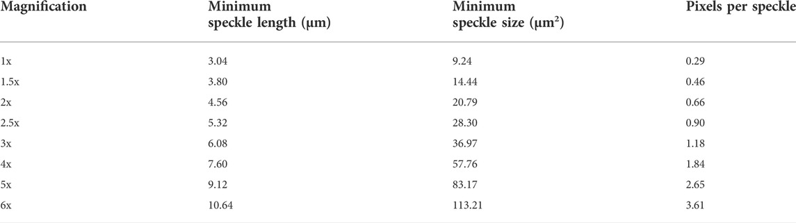
TABLE 1. Minimum speckle length, minimum speckle size and pixels per speckle for each magnification used.

A 200 µm core size MM fiber was used to transmit the laser light to illuminate the static medium. This core size was chosen over the smaller 62.5 µm and the larger 400 µm core sizes because it was deemed to be a size which balanced the tradeoffs between these other sizes - one that was not too small such that the number of observable speckles in the captured image speckle is severely limited and subsequent analysis would be impaired, yet one which was small enough such that it would not impose significant practical limitations on the flexibility of the fiber. Two different static mediums were used – a single-scattering, non-transparent solid iron medium and a multiple-scattering, silica-based tissue-mimicking phantom with ${\mu }_a$ = 0.04 cm⁻¹ and ${\mu }_s^{\prime }$ = 9.6 cm⁻¹. Another 200 µm core size MM fiber, placed at a distance of 15 mm from the source fiber, was used to transmit the backscattered light from the medium to the imaging system. Figure 1A shows a schematic of the setup with the single-scattering iron medium, while Figure 1B shows a schematic of the setup with the multiple-scattering silica-based phantom. A representative image of the experimental setups is also shown in Supplementary Figure S1A. At each magnification, the exposure time of the CCD camera was varied from 2 to 8 ms (in steps of 2 ms), a range contained within the typical range of exposure times for laser speckle imaging in biomedical applications (1–10 ms) [16]. The frame rate was kept constant at 100 fps. For each configuration of magnification and exposure time, the laser power and CCD gain were appropriately tuned to prevent the intensities of the CCD pixels in the illumination area from reaching the saturation threshold. Generally, the laser power was kept within the range of <20 mW.

FIGURE 1

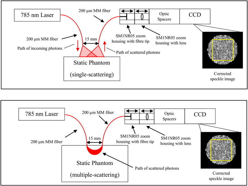
FIGURE 1. Schematic of the setup used in the static experiment. 785 nm laser light was delivered via a 200 μm MM fiber to illuminate a static phantom, and the backscattered light was transmitted via another 200 μm MM fiber placed 15 mm away to a CCD which captured the speckle image. SM1NR05 zoom housings containing the fiber tip and lens, along with optic spacers, were used to adjust the magnification of the system. The raw image captured by the CCD was then corrected against a normalized background pattern to obtain a corrected speckle image. The yellow box in the corrected speckle image shows the area in the speckle pattern used for the calculation of $1/K^2$. (A) (top) For the single-scattering medium (a non-transparent iron block), the fiber transmitting the laser light and detection fiber were placed a distance away from the phantom to allow the scattered photons to enter the detection fiber and subsequently hit the CCD pixel array. (B) (bottom) For the multiple-scattering medium (a silica-based, tissue-mimicking phantom), the fiber transmitting the laser light and detection fiber were placed against the surface of the phantom for better detection of the multiple-scattering events.

A representative speckle image was obtained at each magnification, and these are shown in Figures 2A–H.

FIGURE 2

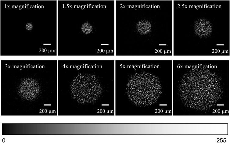
FIGURE 2. (A) (top row, leftmost) Corrected speckle image at 1× magnification. (B) (top row, 2nd from left) Corrected speckle image at 1.5× magnification. (C) (top row, 2nd from right) Corrected speckle image at 2× magnification. (D) (top row, rightmost) Corrected speckle image at 2.5× magnification. (E) (2nd row, leftmost) Corrected speckle image at 3× magnification. (F) (2nd row, 2nd from left) Corrected speckle image at 4× magnification. (G) (2nd row, 2nd from right) Corrected speckle image at 5× magnification. (H) (2nd row, rightmost) Corrected speckle image at 6× magnification. The brightness of each image has been adjusted to highlight the speckle pattern. The colour bar shows the range of pixel intensities from 0 to 255 (8-bit).

At each magnification and exposure time, $1/K^2$ readings were recorded over 5 min to determine average values. To remove the non-uniform background intensity from the MM fiber tip, the speckle images were adjusted by being divided by the background intensity profile which was averaged by 6,000 pre-recorded images. After the data was collected, the mean $1/K^2$ values were calculated and plotted against the number of pixels per speckle. Figures 3A,B show the plots for the single- and multiple-scattering mediums, respectively.

FIGURE 3

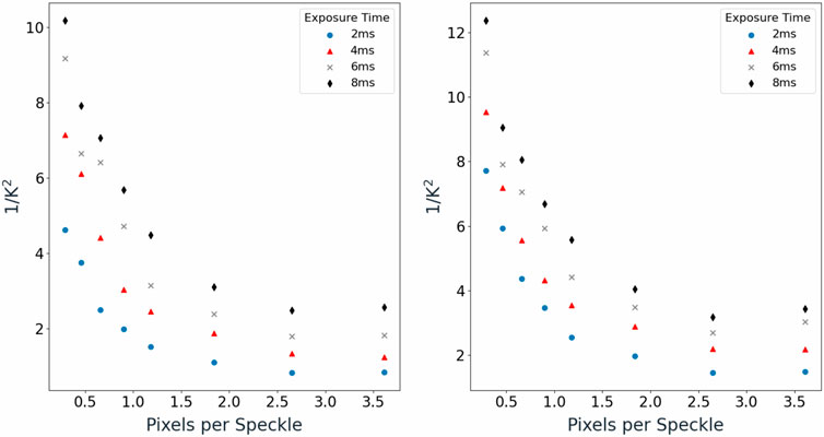
FIGURE 3. (A) (left) Mean $1/K^2$ values vs. Pixels per Speckle over different exposure times for the single-scattering medium. (B) (right) Mean $1/K^2$ values vs. Pixels per Speckle over different exposure times for the multiple-scattering medium. The associated error bars for each point were omitted for better visibility. These can be found in Supplementary Figures S2A,B.

The general trend between $1/K^2$ and the number of pixels per speckle resembled a decaying exponential for both mediums, with values flattening from 2.65 pixels per speckle onwards. Both sets of data agree well with the trend observed by Kirkpatrick et al. [29] between global speckle contrast and pixels per speckle using LSCI, as well as their observation of the distorted $K$ values when the speckle pattern is sampled at a rate below the Nyquist sampling rate; below this rate, the $1/K^2$ values vary despite the illuminated surface remaining static, due to changes of $\beta$. To gain a clearer picture of the relationship between $1/K^2$ and the number of pixels per speckle below the Nyquist rate, the recorded $1/K^2$ values up to a pixels per speckle value of 1.84 were plotted against the reciprocal of pixels per speckle (1/pixels per speckle) to determine the goodness of fit. Figures 4A,B show the plots for the single- and multiple-scattering mediums respectively.

FIGURE 4

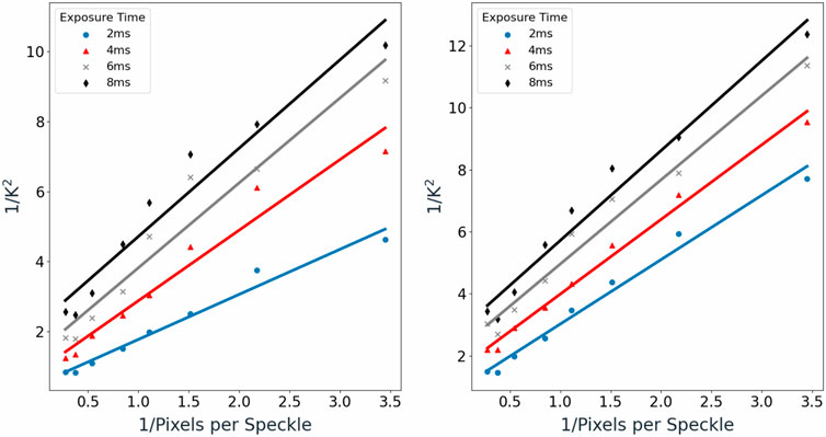
FIGURE 4. (A) (left) Mean $1/K^2$ values vs. 1/Pixels per Speckle over different exposure times for the single-scattering medium. (B) (right) mean Mean $1/K^2$ values vs. 1/Pixels per Speckle over different exposure times for the multiple-scattering medium. The associated error bars for each point were omitted for better visibility. These can be found in Supplementary Figures S3A,B.

Good linear fitting was observed, with coefficient of determination (R²) values ranging from 0.92 to 0.97 for the single-scattering medium and 0.97 to 0.99 for the multiple-scattering medium.

Knowing that $1/K^2$ is linearly correlated with 1/β from Eq. 2 and observing that $1/K^2$ correlates well with 1/pixels per speckle, we conclude that it is likely that $\beta$ is linearly proportional to pixels per speckle. This experimental relationship between $\beta$ and pixels per speckle can help to estimate $\beta$ when the magnification of the imaging system or number of pixels per speckle is below the Nyquist sampling rate.

Based on Figures 3A,B, exposure time was also observed to have a positive relationship with $1/K^2$ at each pixels per speckle value.

4 Experiment on dynamic phantom

A separate experiment was performed to determine the effect of the number of pixels per speckle and CCD camera exposure time on the sensitivity of the $1/K^2$ values to flow. This was measured by the gradient of the regression line of the measured $1/K^2$ flow readings against a range of actual flow rates under dynamic flow conditions. For this, a flow phantom filled with glass beads was used instead of a static medium - the glass beads served to randomize the direction of flow. Both the fiber transmitting the laser light and the detecting fiber were placed against the surface of the flow phantom which had optical properties ${\mu }_a$ = 0.04 cm⁻¹ and ${\mu }_s^{\prime }$ = 9.6 cm⁻¹. A representative image of the experimental setup is shown in Supplementary Figure S1B. A source-detector separation of 8 mm was used, and a frame rate of 80 fps was used. All other elements of the set-up remained the same as in the previous experiment. A 2% Lipofundin solution (B. Braun, Germany), which has optical properties similar to those of blood, was pumped through the flow phantom using a peristaltic pump at flow rates ranging from 0.1 ml/s to 1 ml/s (in steps of 0.1 ml/s). Like in the previous experiment, the number of pixels per speckle was varied by varying the magnification of the imaging system. The magnifications used ranged across 1x, 2x, 3x and 4x, corresponding to pixels per speckle values of 0.29, 0.66, 1.18 and 1.84 respectively. The CCD camera exposure times used ranged from 2 to 8 ms (in steps of 2 ms). As before, the laser power and gain were also adjusted to prevent saturation of the CCD pixels in each configuration. The laser power was maintained between 25 and 40 mW.

$1/K^2$ values were recorded for 30 s at each flow rate under each magnification (pixels per speckle value) and exposure time. The recorded data was then smoothened with a moving average window, following which the mean and standard deviation of the data were calculated. Figures 5A,B show plots of smoothened and mean $1/K^2$ values for each flow rate respectively, under a pixels per speckle value of 0.29 and exposure time of 2 ms, and Figure 5C shows the regression lines for the mean $1/K^2$ values against flow rate for each CCD camera exposure time, also under a pixels per speckle value of 0.29.

FIGURE 5

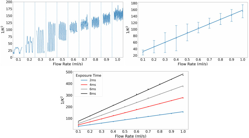
FIGURE 5. (A) (top left) Smoothened $1/K^2$ values against flow rate using a pixels per speckle value of 0.29 and CCD camera exposure time of 2 ms. (B) (top right) Mean $1/K^2$ values with error bars representing standard deviation against flow rate using a pixels per speckle value of 0.29 and CCD camera exposure time of 2 ms. (C) (bottom) Regression lines for mean $1/K^2$ values against flow rate for CCD camera exposure times of 2 ms, 4 ms, 6 ms and 8 ms, also under a pixels per speckle value of 0.29. The associated error bars for each point in (C) were omitted for better visibility. These can be found in Supplementary Figure S4.

As seen in Figure 5A, the periodic changes in flow rate produced by the peristaltic pump were detected by the CCD camera and reflected in the fluctuating $1/K^2$ values, with the frequency of fluctuations and $1/K^2$ values increasing with the flow rate. A strong linear relationship was observed between the mean $1/K^2$ values and flow rate (Figure 5B), and this was similarly observed in the plots for all pixels per speckle values and exposure times used, with coefficient of determination (R²) values ranging from 0.95 to 0.999 (Table 2, Supplementary Figures S5A–P). This confirmed the fact that the range of flow rates used corresponded to the range of $\alpha D_b$ values for which $1/K^2$ is linear [12]. One might notice that the error bars in Figure 5B and Supplementary Figures S5A–P increase substantially from flow rates of 0.1 ml/s to 0.5 ml/s then become small again from 0.6 ml/s onwards. These error bars represent the standard deviation derived from the range of flow values produced by the peristaltic pump at each flow rate; the amplitudes of the flow oscillations increased significantly at lower pumping frequencies, but became small at higher pumping frequencies because of the flow momentum generated. A slight decrease in the R² values was observed at higher pixels per speckle values (higher magnifications of the imaging system) due to the tapering off of the increase in $1/K^2$ values at the higher flow rates. This can be attributed to the lower signal to noise ratio (SNR) at the higher magnifications. Higher magnifications cause the detected signal to be spread to more pixels, reducing the signal intensity received by each pixel significantly.

TABLE 2

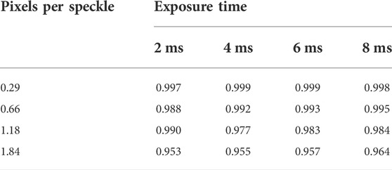
TABLE 2. R² values for the plots of the obtained mean $1/K^2$ values against flow rate for the different pixels per speckle values and exposure times used.

Increasing the exposure time of the CCD camera resulted in an increase in the sensitivity of the system, as seen in the increasing gradients of the regression lines of the mean $1/K^2$ values against flow rate in Figure 5C. Through experimental observation, we conclude that within this exposure time range, longer exposure times result in higher sensitivities of the $1/K^2$ values to flow. However, longer exposure times also result in decreased measurement rates. For applications requiring high temporal resolutions, researchers need to keep a balance between sensitivity and measurement rate.

The magnitudes of the gradients were also calculated for the other configurations of pixels per speckle and exposure time. These are plotted in Figure 6.

FIGURE 6

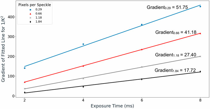
FIGURE 6. Gradient values of the regression lines fitted between $1/K^2$ and flow rate for different Pixels per Speckle values vs. Exposure Time.

A linear relationship between the magnitude of the gradient and exposure time was observed across all pixels per speckle values, with coefficient of determination (R²) values exceeding 0.99 for all cases. The gradient for $1/K^2$ vs. flow rate also exhibited an inverse relationship with the number of pixels per speckle, validating the theoretical relationship; from Eq. 2, a lower $\beta$ value will result in a higher $1/K^2$ reading at a given exposure time. Practically, these results suggest that both the CCD camera exposure time and number of pixels per speckle influence the sensitivity of the DSPF system to flow measurements, and both parameters will need to be controlled for different sensitivity and flow range requirements.

5 Discussion

We believe the results presented herein may offer a better theoretical understanding of diffuse laser speckle analysis. The proposed linear relationship between pixels per speckle and $\beta$ gives further characterization to the parameter $\beta$, providing an understanding of how it is affected by speckle size in the case of undersampling. With this understanding, researchers using DSPF and other laser speckle-based flow imaging techniques may better estimate $\beta$ and tune the parameters of the laser speckle contrast model to control the output flow readings ($1/K^2$). This may in turn allow better calibration of their instrumentation. As a disclaimer, however, although we propose this linear relationship, we were unable to deduce an explicit mathematical relationship between pixels per speckle and $\beta$. This would require more mathematical analysis and experimental validation, which can be explored in future studies.

The parameters used in our study were tailored towards the use of DSPF systems in biomedical applications. The range of exposure times studied was within the normal range used in biomedical applications [16], and the pixels per speckle values used were chosen based on practically feasible magnifications of the imaging system. We deemed magnifications of the imaging system from 1x to 4x for flow setups to be practically feasible as they did not require excessively thick lens or large image distances. Imaging magnifications lower than 1x were not experimented with, although these might be beneficial because they cause the energy from the backscattered photons to be concentrated onto a smaller area on the CCD array, improving the SNR. For the purposes of this study, however, we believed that an imaging magnification of 1x was sufficiently small. The 1x magnification is also arguably the most convenient magnification that can be used, given that it can involve just placing the fiber tip at the CCD array, removing the need for lenses and space to accommodate larger image distances. This may be especially useful for sensors for which compactness is a key requirement.

6 Conclusion

In this study, we present results of experimental characterization tests on the recently developed DSPF technique. Because DSPF uses a MM detection fiber which captures multiple speckles in a single image frame and renders speckle size a parameter which affects the output flow readings, we designed and implemented a lens module that could allow the magnification of the imaging system to be changed easily to study the effect of speckle size. We have been able to determine the relationship between $\beta$ and the number of pixels per speckle, as well as the effects of the number of pixels per speckle and exposure time on the sensitivity of $1/K^2$ to flow measurements. Through our experimental results, it is likely that $\beta$ is linearly related to the number of pixels per speckle when the magnification of the imaging system is below the Nyquist sampling rate for laser speckles. Our results indicated that DSPF’s flow measurement capability remained valid even when the Nyquist sampling rate of laser speckles was not reached, when the number of pixels per speckle was equal to or higher than 0.29 (magnification of the imaging system is 1x). With this knowledge, researchers may choose an optimal speckle size for specific applications. Separately, exposure time was also found to be positively related to $1/K^2$ in no-flow setups. In addition, we also found that the sensitivity of the DSPF system to flow would increase if a longer exposure time were used, within the range of 2–8 ms. However, higher exposure times would result in a decreased measurement rate, which may be undesirable. The sensitivity of the system also exhibited an inverse relationship with the number of pixels per speckle, thus implying that both exposure time and the number of pixels per speckle need to be controlled for specific sensitivity requirements. The reported results bear useful implications for practical applications, and it is hoped that these results may continue to further theoretical research in laser speckle analysis and support the development of instrumentation for practical use.

Data availability statement

The original contributions presented in the study are included in the article/Supplementary Material, further inquiries can be directed to the corresponding authors.

Author contributions

Conceptualization, RB; methodology, RB; software, RB; validation, TC; formal analysis, TC; investigation, TC; resources, MO; data curation, TC and RB; writing—original draft preparation, TC; writing—review and editing, RZ and RB; visualization, TC; supervision, RB; project administration, RB; funding acquisition, RB. All authors have read and agreed to the published version of the manuscript.

Funding

This research was funded by Agency of Science, Technology and Research (A*STAR) under its Industry Alignment Fund prepositioning program (IAF-PP), Award H19/01/a0/0EE9 and BMRC Central Research Fund (UIBR) 2021.

Conflict of interest

The authors declare that the research was conducted in the absence of any commercial or financial relationships that could be construed as a potential conflict of interest.

Publisher’s note

All claims expressed in this article are solely those of the authors and do not necessarily represent those of their affiliated organizations, or those of the publisher, the editors and the reviewers. Any product that may be evaluated in this article, or claim that may be made by its manufacturer, is not guaranteed or endorsed by the publisher.

Supplementary material

The Supplementary Material for this article can be found online at: https://www.frontiersin.org/articles/10.3389/fphy.2022.1006484/full#supplementary-material

References

1. Nakano H, Okazaki K, Ajiro Y, Suzuki T, Oba K. Clinical usefulness of the common carotid artery blood flow velocity ratio as measured by an ultrasonic quantitative flow measurement system: Evaluation with respect to prevalence of ischemic heart disease. J Nippon Med Sch (2001) 68(6):482–9. doi:10.1272/jnms.68.482

PubMed Abstract | CrossRef Full Text | Google Scholar

2. Xiao M, Li Q, Feng H, Zhang L, Chen Y. Neural vascular mechanism for the cerebral blood flow autoregulation after hemorrhagic stroke. Neural plasticity (2017) 2017:1–12. doi:10.1155/2017/5819514

CrossRef Full Text | Google Scholar

3. Caplan LR. Caplan's stroke. Cambridge University Press (2016).

Google Scholar

4. Pendsey SP. Understanding diabetic foot. Int J Diabetes Dev Ctries (2010) 30(2):75–9. doi:10.4103/0973-3930.62596

PubMed Abstract | CrossRef Full Text | Google Scholar

5. Han P, Li L, Zhang H, Guan L, Marques C, Savović S, et al. Low-cost plastic optical fiber sensor embedded in mattress for sleep performance monitoring. Opt Fiber Tech (2021) 64:102541. doi:10.1016/j.yofte.2021.102541

CrossRef Full Text | Google Scholar

6. Leal-Junior AG, Díaz CR, Leitão C, Pontes MJ, Marques C, Frizera A. Polymer optical fiber-based sensor for simultaneous measurement of breath and heart rate under dynamic movements. Opt Laser Tech (2019) 109:429–36. doi:10.1016/j.optlastec.2018.08.036

CrossRef Full Text | Google Scholar

7. Peters K. Polymer optical fiber sensors—a review. Smart materials and structures. 2010;20(1):013002.

CrossRef Full Text | Google Scholar

8. Bi R, Du Y, Singh G, Ho J-H, Zhang S, Attia ABE, et al. Fast pulsatile blood flow measurement in deep tissue through a multimode detection fiber. J Biomed Opt (2020) 25(5):1–10.

PubMed Abstract | CrossRef Full Text | Google Scholar

9. Durduran T, Choe R, Baker WB, Yodh AG. Diffuse optics for tissue monitoring and tomography. Rep Prog Phys (2010) 73(7):076701. doi:10.1088/0034-4885/73/7/076701

PubMed Abstract | CrossRef Full Text | Google Scholar

10. Buckley EM, Parthasarathy AB, Grant PE, Yodh AG, Franceschini MA. Diffuse correlation spectroscopy for measurement of cerebral blood flow: Future prospects. Neurophotonics (2014) 1(1):011009. doi:10.1117/1.nph.1.1.011009

PubMed Abstract | CrossRef Full Text | Google Scholar

11. Bi R, Dong J, Lee K. Deep tissue flowmetry based on diffuse speckle contrast analysis. Opt Lett (2013) 38(9):1401–3. doi:10.1364/ol.38.001401

PubMed Abstract | CrossRef Full Text | Google Scholar

12. Bi R, Dong J, Lee K. Multi-channel deep tissue flowmetry based on temporal diffuse speckle contrast analysis. Opt Express (2013) 21(19):22854–61. doi:10.1364/oe.21.022854

PubMed Abstract | CrossRef Full Text | Google Scholar

13. Yeo C, Jung H, Lee K, Song C. Low frequency oscillations assessed by diffuse speckle contrast analysis for foot angiosome concept. Sci Rep (2020) 10(1):17153–14. doi:10.1038/s41598-020-73604-0

PubMed Abstract | CrossRef Full Text | Google Scholar

14. Yeo C, Kim H, Song C. Cerebral blood flow monitoring by diffuse speckle contrast analysis during MCAO surgery in the rat. Curr Opt Photon (2017) 1(5):433–9.

Google Scholar

15. Teng Z, Gao F, Xia H, Chen W, Li C. In vivo pulse wave measurement through a multimode fiber diffuse speckle analysis system. Front Phys (2020) 8(613342). doi:10.3389/fphy.2020.613342

CrossRef Full Text | Google Scholar

16. Boas DA, Dunn AK. Laser speckle contrast imaging in biomedical optics. J Biomed Opt (2010) 15(1):011109. doi:10.1117/1.3285504

PubMed Abstract | CrossRef Full Text | Google Scholar

17. Yu G. Diffuse correlation spectroscopy (DCS): A diagnostic tool for assessing tissue blood flow in vascular-related diseases and therapies. Curr Med Imaging Rev (2012) 8(3):194–210. doi:10.2174/157340512803759875

CrossRef Full Text | Google Scholar

18. Obeid A, Barnett N, Dougherty G, Ward G. A critical review of laser Doppler flowmetry. J Med Eng Technol (1990) 14(5):178–81. doi:10.3109/03091909009009955

PubMed Abstract | CrossRef Full Text | Google Scholar

19. Liu J, Zhang H, Lu J, Ni X, Shen Z. Quantitative model of diffuse speckle contrast analysis for flow measurement. J Biomed Opt (2017) 22(7):076016. doi:10.1117/1.jbo.22.7.076016

PubMed Abstract | CrossRef Full Text | Google Scholar

20. Liu J, Zhang H, Lu J, Ni X, Shen Z. Simultaneously extracting multiple parameters via multi-distance and multi-exposure diffuse speckle contrast analysis. Biomed Opt Express (2017) 8(10):4537–50. doi:10.1364/boe.8.004537

PubMed Abstract | CrossRef Full Text | Google Scholar

21. Leal-Junior AG, Frizera A, Marques C, Pontes MJ. Optical fiber specklegram sensors for mechanical measurements: A review. IEEE Sens J (2019) 20(2):569–76. doi:10.1109/jsen.2019.2944906

CrossRef Full Text | Google Scholar

22. Sironi L, D'Alfonso L, Bouzin M, Ceffa NG, Collini M, Chirico G, et al. Optical blood flow measurement in microcirculatory systems (2016).

Google Scholar

23. Briers JD. Laser Doppler, speckle and related techniques for blood perfusion mapping and imaging. Physiol Meas (2001) 22(4):R35–66. doi:10.1088/0967-3334/22/4/201

PubMed Abstract | CrossRef Full Text | Google Scholar

24. Fercher A, Briers JD. Flow visualization by means of single-exposure speckle photography. Opt Commun (1981) 37(5):326–30. doi:10.1016/0030-4018(81)90428-4

CrossRef Full Text | Google Scholar

25. Briers JD, Webster S. Laser speckle contrast analysis (LASCA): A nonscanning, full-field technique for monitoring capillary blood flow. J Biomed Opt (1996) 1(2):174–9. doi:10.1117/12.231359

PubMed Abstract | CrossRef Full Text | Google Scholar

26. Bi R, Dong J, Poh CL, Lee K. Optical methods for blood perfusion measurement—Theoretical comparison among four different modalities. J Opt Soc Am A (2015) 32(5):860–6. doi:10.1364/josaa.32.000860

PubMed Abstract | CrossRef Full Text | Google Scholar

27. Parthasarathy AB, Tom WJ, Gopal A, Zhang X, Dunn AK. Robust flow measurement with multi-exposure speckle imaging. Opt Express (2008) 16(3):1975–89. doi:10.1364/oe.16.001975

PubMed Abstract | CrossRef Full Text | Google Scholar

28. Lemieux P-A, Durian D. Investigating non-Gaussian scattering processes by using nth-order intensity correlation functions. J Opt Soc Am A (1999) 16(7):1651–64. doi:10.1364/josaa.16.001651

CrossRef Full Text | Google Scholar

29. Kirkpatrick SJ, Duncan DD, Wells-Gray EM. Detrimental effects of speckle-pixel size matching in laser speckle contrast imaging. Opt Lett (2008) 33(24):2886–8. doi:10.1364/ol.33.002886

PubMed Abstract | CrossRef Full Text | Google Scholar