A note on the slip effects of an Oldroyd 6-constant fluid: Optimal homotopy asymptotic method

We study here the effectiveness of the optimal homotopy asymptotic method (OHAM) in solving non-linear differential equations of non-Newtonian fluids. To this consequence, we consider the Oldroyd 6-constant fluid when it demonstrates slippage between the plate and fluid generating non-linear boundary value problems. The problems of plane Couette flow, generalized Couette flow, and plane Poiseuille flow are considered. Graphs of the results are plotted to show the performance of the method in terms of velocity profile. It is observed that the method is quite easy to implement, having latent potential to handle such kinds of non-linear problems and yield accurate results at minimum to low computational work.

1 Introduction

Analysis of the traditional spatial patterns from animate and inanimate natural processes has been a source of marvelous attraction since the early stages of scientific exploration and in recent advancements. Experimental investigation and quantitative understanding of the essential mechanisms are a rather recent achievement, which has been possible only due to firm determination, rationale approach, and rigorous effort in the course of research in non-linear physics and mathematics. While contemplating non-linear phenomena, which appear in a variety of ways, researchers have been facing difficulties at the outset.

In fluid mechanics, the effect of slip conditions on the behavior of flow was first studied by Navier [1]; the Navier–Stokes’s equations, which are the governing equations for Newtonian fluid flow, describe it well. The calculations about slip boundary conditions were based on molecular weights. But rheological complex fluids such as polymeric solutions, blood, paint, shampoo, starch, certain oils, and grease, whose flow behavior and characteristics cannot be described at all by the Navier–Stokes’s equations, having non-linear relationship between shear stress and strain rate, are called non-Newtonian fluids. Their extensive use in the oil industry, chemical industry, food industry, construction and power engineering, and commercial and rheological applications has led to the emergence of several theories and rigorous work in non-Newtonian fluid mechanics.

Rajagopal and Bhatnagar [2], Rajagopal [3], Baris [4], Hayat et al [5, 6], and Siddiqui AM et al [7, 8] have tried to explain this behavior of non-Newtonian fluids. Due to important technological and engineering applications, numerous attempts have been made to elucidate the slip phenomena [9–12]. A number of attempts have been made to numerically explain the behavior and concerning parameters of non-Newtonian flow with slip effect [13–17]. Recently, Hayat et al [18] had studied the effect of the slip conditions on the flow of an Oldroyd 6-constant fluid.

The objective of this work is to see the effectiveness of the optimal homotopy asymptotic method (OHAM) by studying and analyzing different parameters of the equations describing 6-constant Oldroyd fluid flow and presenting the solutions in terms of velocity profiles. This method was proposed by Marinca et al. [19]. The advantage of the OHAM is the integrated convergence criteria that is similar to HAM but flexible to a greater extent in implementation. Marinca et al. [20–22] and Iqbal et al. [23–30], in a series of articles, have established the validity, usefulness, simplification, and consistency of the method and acquired reliable solutions of currently significant applications in science and technology. The considered model is present in the literature [18] and has unique characteristics of earlier fluids. The OHAM demonstrates the imbedding potential and tenders a reliable solution for three steady flows (Couette, Poiseuille, and generalized Couette).

2 Governing equations

The governing equation for Oldroyd 6-constant fluid [18] is expressed as

$\frac{du}{dy}+{\alpha }_1{\left(\frac{du}{dy}\right)}^3-\left(yK+{\beta }_1\right)\left[{\alpha }_2{\left(\frac{du}{dy}\right)}^2+R^2\right]=0(1)$

where $K=d\widehat{p}/dx$, $\gamma =\mu /\rho$, $R$ is the Reynolds number, ${\alpha }_1,{\alpha }_2$ are constants, and ${\beta }_1$ is the constant of integration. The laminar flow of an Oldroyd 6-constant fluid between two infinite parallel plates at a fixed distance apart are of three types:

•Plane Couette flow: The lower plate is stationary and the upper plate moves. Flow is due to the motion of the upper plate, since the pressure gradient is zero in the x-direction, i.e., $\widehat{p}=0$ $\left(K=0\right)$ having

$u\left(0\right)-\gamma u^{/}\left(0\right)=0\mathrm{a}\mathrm{n}\mathrm{d}u\left(1\right)+\gamma u^{/}\left(1\right)=1(2)$

•Plane Poiseuille flow: Both the plates are at rest and the flow is due to the pressure gradient in the x-direction, i.e., $\left(K=d\widehat{p}/dx\right)$ having

$u\left(0\right)-\gamma u^{/}\left(0\right)=0\mathrm{a}\mathrm{n}\mathrm{d}u\left(1\right)+\gamma u^{/}\left(1\right)=0(3)$

• Plane Couette–Poiseuille flow: Flow starts due to both the pressure gradient in the x-direction, i.e., $\left(K=d\widehat{p}/dx\right)$ and the motion of the upper plate having

$u\left(0\right)-\gamma u^{/}\left(0\right)=0\mathrm{a}\mathrm{n}\mathrm{d}u\left(1\right)+\gamma u^{/}\left(1\right)=1(4)$

3 Optimal homotopy asymptotic method formulation

The OHAM [19–27, 31, 32] is tested to find the velocity field $u\left(y\right)$ of the governing differential Equation 1 with the slip boundary conditions (2)–(4) given in Section 2. According to the OHAM [19–22, 31], the differential equation can be written as

$A\left(v\left(y\right)\right)+f\left(y\right)=0,y\in \mathrm{\Omega }(5)$

$\mathrm{w}\mathrm{h}\mathrm{e}\mathrm{r}\mathrm{e}\mathrm{\Omega }$ is the domain. Now Equation 5 is decomposed into $A\left(v\right)=L\left(v\right)+N\left(v\right).$ We have the freedom to choose the linear part $L$. According to the OHAM, one can construct an optimal homotopy $\varphi \left(y;p\right):$ $\Omega \times \left[-\mathrm{1,1}\right]\to \mathbb{R}$ which satisfies

$\left(1-p\right)\left\{L\left(\varphi \left(y;p\right)\right)+f\left(y\right)\right\}-H\left(p\right)\left\{A\left(\varphi \left(y;p\right)\right)+f\left(y\right)\right\}=0(6)$

where $p\in \left[\mathrm{0,1}\right]$ is an embedding parameter, $H\left(p\right)=p{C}_1+p^2{C}_2+...$ is a non-zero auxiliary function for $p\ne 0$, $H\left(0\right)=0$, where $C_1,C_{2,}...$ are constants to be determined. Eq. 6 is called optimal homotopy equation. To get an approximate solution, we expand $\varphi \left(y;p,C_i\right)$ in the Taylor series about $p$ in the following manner:

$\varphi \left(y;p,C_i\right)=v_0\left(r,t\right)+{\displaystyle \sum }_{k=1}^{\infty }{v}_k\left(y;C_i\right)p^k,i=\mathrm{1,2},...(7)$

It has been observed that the convergence of the series’ Equation 7 depends upon the auxiliary constants $C_1,C_{2,}...$. If it is convergent at $p=1$, one has

$\underset{\sim }{v}\left(y;C_i\right)=v_0\left(y\right)+{\displaystyle \sum }_{k\ge 1}{v}_k\left(y;C_i\right)(8)$

Substituting Equation 8 into Equation 5 results in the following expression for the residual:

$R\left(y;C_i\right)=L(\underset{\sim }{v}\left(y;C_i\right))+f\left(y\right)+N(\underset{\sim }{v}\left(y;C_i\right))(9)$

$\mathrm{I}\mathrm{f}R\left(y;C_i\right)=0,\mathrm{t}\mathrm{h}\mathrm{e}\mathrm{n}\underset{\sim }{v}\left(y;C_i\right)$ will be the exact solution. This does not generally happen, especially in non-linear problems. For determining the optimal values of the convergence-control parameters, $C_i,i=\mathrm{1,2},...,m$, one can see the [23–29].

3.1 Plane Couette flow

Now, the OHAM is applied to give an explicit, uniformly valid, analytic solution to the governing differential Equation 1, and the slip conditions (2). The OHAM constructed zeroth-order deformation equation as

$\frac{d{u}_0}{dy}-R^2{\beta }_1=0\hspace{0.17em}{u}_0\left(0\right)-\gamma u_0^{/}\left(0\right)=0(10)$

$u_0\left(y\right)=R^2{\beta }_1\left(y+\gamma \right)$ is the solution of Equation 10. By applying the boundary condition $u_0\left(1\right)+\gamma u_0^{/}\left(1\right)=1$, one can get ${\beta }_1=1/R^2\left(1+2\gamma \right)$. Therefore,

$u_0\left(y\right)=\frac{y+\gamma }{1+2\gamma }(11)$

The first-order deformation equation is constructed as

$\begin{array}{l}\frac{d{u}_1}{dy}=\left(1+C_1\right)\frac{d{u}_0}{dy}-C_1{\alpha }_2{\beta }_1{\left(\frac{d{u}_0}{dy}\right)}^2+C_1{\alpha }_1{\left(\frac{d{u}_0}{dy}\right)}^3-\left(1+C_1\right)R^2{\beta }_1\\ u_1\left(0\right)-\gamma u_1^{/}\left(0\right)=0\end{array}(12)$

The first-order solution is obtained by solving Equation 12 using zeroth order solution (11) and ${\beta }_1=1/R^2\left(1+2\gamma \right)$ as

$u_1\left(y\right)=\frac{\left(y+\gamma \right)\left({\left(R+2R\gamma \right)}^2+C_1\left(R^2{\alpha }_1-{\alpha }_2\right)\right)}{R^2{\left(1+2\gamma \right)}^3}(13)$

Hence, by adding the zeroth-order and first-order solutions, and other higher order solutions if necessary, one gets

$u\left(y\right)=\frac{\left(y+\gamma \right)\left(2{\left(R+2R\gamma \right)}^2+C_1\left(R^2{\alpha }_1-{\alpha }_2\right)\right)}{R^2{\left(1+2\gamma \right)}^3}(14)$

Using the procedure mentioned in [19–27, 31, 32], for the constant $C_1$, an optimal value of the auxiliary constants is presented in Table 1 for different slip parameters.

TABLE 1

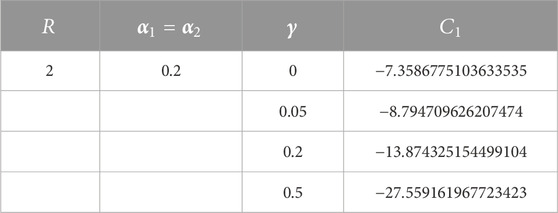
TABLE 1. Optimal values of auxiliary constant $C_1$ for different slip parameters (plane Couette flow).

3.2 Plane Poiseuille flow

An explicit analytic solution of the governing differential Equation 1, and the slip conditions (3) for plane Poiseuille flow is determined. The OHAM constructed zeroth-order deformation equation is

$\frac{d{u}_0}{dy}-K{R}^{2}y-R^2{\beta }_1=0u_0\left(0\right)-\gamma u_0^{/}\left(0\right)=0(15)$

The solution of zeroth-order deformation in Equation 15 is given as

$u_0\left(y\right)=\frac{K{R}^2{y}^2+2R^2{\beta }_1\left(y+\gamma \right)}{2}(16)$

Now, by using the condition $u_0\left(1\right)+\gamma u_0^{/}\left(1\right)=0$ in Equation 16, one can get the integration constant ${\beta }_1=-K/2$. By using the value of ${\beta }_1$ in Equation 16, one can get the zeroth-order solution as

$u_0\left(y\right)=\frac{K{R}^2\left(y^2-y-\gamma \right)}{2}(17)$

The first-order deformation equation is

$\begin{array}{l}\frac{d{u}_1}{dy}=\left(1+C_1\right)\frac{d{u}_0}{dy}-C_1{\alpha }_2\left(Ky+{\beta }_1\right){\left(\frac{d{u}_0}{dy}\right)}^2\\ +C_1{\alpha }_1{\left(\frac{d{u}_0}{dy}\right)}^3-\left(1+C_1\right)\left(K{R}^{2}y+R^2{\beta }_1\right)\\ u_1\left(0\right)-\gamma u_1^{/}\left(0\right)=0\end{array}(18)$

The first-order solution is obtained by solving Equation 18 using the zeroth-order solution (17) and ${\beta }_1=-K/2$ as

$u_1\left(y\right)=\frac{1}{8}{K}^3{R}^4\left(-y+3y^2-4y^3+2y^4-\gamma \right)C_1\left(R^2{\alpha }_1-{\alpha }_2\right)(19)$

By adding the zeroth-order and first-order solutions given in Eqs. 7, 18, one gets

$\begin{array}{l}u\left(y\right)=\frac{1}{2}K{R}^2\left(-y+y^2-\gamma \right)\\ +\frac{K^3{R}^4}{8}\left(-y+3y^2-4y^3+2y^4-\gamma \right)C_1\left(R^2{\alpha }_1-{\alpha }_2\right)\end{array}(20)$

Using the procedure “Least Squares Method” mentioned in [19–22, 31], for constant $C_1$, the optimal value of the auxiliary constant for the different slip parameters is $C_1=-0.7380617718616882$.

3.3 Plane Couette–Poiseuille flow

The solution of the governing differential Equation 1, and the slip condition (4) for plane Couette–Poiseuille flow is determined. The OHAM constructed zeroth-order deformation equation is

$\frac{d{u}_0}{dy}-K{R}^{2}y-R^2{\beta }_1=0u_0\left(0\right)-\gamma u_0^{/}\left(0\right)=0(21)$

Eq. 21 implies the zeroth-order solution as

$u_0\left(y\right)=\frac{K{R}^2{y}^2+2R^2{\beta }_1\left(y+\gamma \right)}{2}(22)$

By using the condition $u_0\left(1\right)+\gamma u_0^{/}\left(1\right)=1$ in Equation 22, one gets

${\beta }_1=\frac{2-K{R}^2\left(1+2\gamma \right)}{2R^2\left(1+2\gamma \right)}(23)$

By putting this value of the integration constant ${\beta }_1$ in Equation 22, one gets the zeroth-order solution as

$u_0\left(y\right)=\frac{K{R}^2{y}^2}{2}+\frac{\left(2-K{R}^2\left(1+2\gamma \right)\right)\left(y+\gamma \right)}{2\left(1+2\gamma \right)}(24)$

The first-order deformation equation is given as

$\begin{array}{l}\frac{d{u}_1}{dy}=\left(1+C_1\right)\frac{d{u}_0}{dy}-C_1{\alpha }_2\left(Ky+{\beta }_1\right){\left(\frac{d{u}_0}{dy}\right)}^2\\ +C_1{\alpha }_1{\left(\frac{d{u}_0}{dy}\right)}^3-\left(1+C_1\right)\left(K{R}^{2}y+R^2{\beta }_1\right)\\ u_1\left(0\right)-\gamma u_1^{/}\left(0\right)=0\end{array}(25)$

The first-order solution is obtained by solving Equation 25 using the zeroth-order solution (24) and ${\beta }_1$ given in Equation 23 as

$u_1\left(y\right)=\frac{C_1\left(R^2{\alpha }_1-{\alpha }_2\right)}{8R^2{\left(1+2\gamma \right)}^3}\left(\begin{array}{l}2R^6{y}^4{\left(K+2K\gamma \right)}^3-\left(y+\gamma \right){\left(-2+K{R}^2\left(1+2\gamma \right)\right)}^3\\ -4R^4{y}^3{\left(K+2K\gamma \right)}^2\left(-2+K{R}^2\left(1+2\gamma \right)\right)\\ +3\mathrm{K}{R}^2{y}^2\left(1+2\gamma \right){\left(-2+K{R}^2\left(1+2\gamma \right)\right)}^2\end{array}\right)(26)$

By adding the zeroth-order and first-order solutions given in Eqs. 24, 26, one gets

$\begin{array}{l}u\left(y\right)=\frac{K{R}^2{y}^2}{2}+\frac{\left(2-K{R}^2\left(1+2\gamma \right)\right)\left(y+\gamma \right)}{2\left(1+2\gamma \right)}\\ +\frac{C_1\left(R^2{\alpha }_1-{\alpha }_2\right)}{8R^2{\left(1+2\gamma \right)}^3}\left(\begin{array}{l}2R^6{y}^4{\left(K+2K\gamma \right)}^3-\left(y+\gamma \right){\left(-2+K{R}^2\left(1+2\gamma \right)\right)}^3\\ -4R^4{y}^3{\left(K+2K\gamma \right)}^2\left(-2+K{R}^2\left(1+2\gamma \right)\right)\\ +3\mathrm{K}{R}^2{y}^2\left(1+2\gamma \right){\left(-2+K{R}^2\left(1+2\gamma \right)\right)}^2\end{array}\right)\end{array}(27)$

Using the procedure mentioned in [19–22, 31], for the constant $C_1$, the optimal values of the auxiliary constants are presented in Table 2 for different slip parameters.

TABLE 2

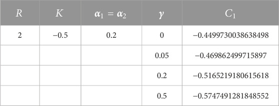
TABLE 2. Optimal values of auxiliary constant $C_1$ for different slip parameters (plane Couette–Poiseuille flow).

4 Results and discussions

Figure 1, Figure 2, and Figure 3 present the velocity profile $u\left(y\right)$ of the plane Couette, plane Poiseuille, and plane Couette–Poiseuille flow for various values of the slip parameter $\gamma =0.0,0.05,0.2,\mathrm{a}\mathrm{n}\mathrm{d}0.5$. It is observed from Figure 1 and Figure 3 that the velocity increases near the fixed plate and decreases near the moving plate as $\gamma$ increases. The solution exhibited in Figure 2 shows that the $u\left(y\right)$ velocity field increases with increase in $\gamma$. The first-order OHAM results are in complete agreement with the HAM solutions [18]. The results show the reliability and potential of the method.

FIGURE 1

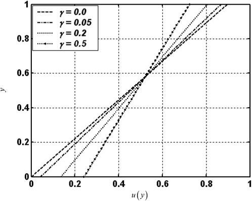
FIGURE 1. Effect of the slip parameter $\gamma$ on the dimensionless velocity profile $u\left(y\right)$ using OHAM for plane Couette flow.

FIGURE 2

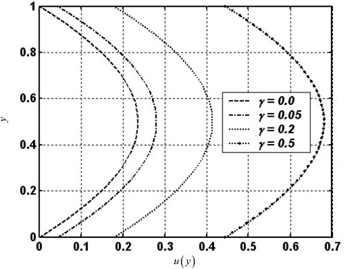
FIGURE 2. Effect of the slip parameter $\gamma$ on the dimensionless velocity profile $u\left(y\right)$ using OHAM for plane Poiseuille flow.

FIGURE 3

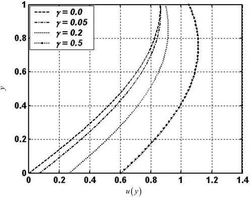
FIGURE 3. Effect of the slip parameter $\gamma$ on the dimensionless velocity field $u\left(y\right)$ using OHAM for plane Couette–Poiseuille flow.

5 Conclusion

In this presentation, Oldroyd 6-constant fluid flow and its response for different slip conditions are discussed for three non-linear boundary value problems. The OHAM is successfully applied to study the constant viscosity models, namely, plane Couette flow, plane Poiseuille flow, and plane Couette–Poiseuille flow for velocity profiles. Graphs are plotted to show the performance of the method in terms of the velocity profiles. This method provides a convenient way to control the convergence by optimally determining the auxiliary constants. The results reveal that the method is precise, effective, and easy to use for non-linear differential equations for Oldroyd 6-constant type fluids.

Data availability statement

The original contributions presented in the study are included in the article/supplementary material; further inquiries can be directed to the corresponding author.

Author contributions

SI and TM have investigated and solved the problem. MS Shah has written the manuscript.

Conflict of interest

The authors declare that the research was conducted in the absence of any commercial or financial relationships that could be construed as a potential conflict of interest.

Publisher’s note

All claims expressed in this article are solely those of the authors and do not necessarily represent those of their affiliated organizations, or those of the publisher, editors, and reviewers. Any product that may be evaluated in this article, or claim that may be made by its manufacturer, is not guaranteed or endorsed by the publisher.

References

1. Navier M. Memoire sur les Lois du mouvement des fluides. Mem L’acad Sci L’inst France (1823) 6:389–440.

Google Scholar

2. Rajagopal KR, Bhatnager RK. Exact solutions for some simple flows of an Oldroyd-B fluid. Acta Mechanica (1995) 113:233–9. doi:10.1007/bf01212645

CrossRef Full Text | Google Scholar

3. Rajagopal KR. On an exact solutions for the flows of an Oldroyd-B fluid. Bull.Tech.Univ.Istanbul. (1996) 49:617–23.

Google Scholar

4. Baris S. Flow of an Oldroyd 6-constant fluid between intersecting planes, one of which is moving. Acta Mechanica (2001) 147:125–35. doi:10.1007/bf01182357

CrossRef Full Text | Google Scholar

5. Hayat T, Siddiqui AM, Asghar S. Some simple flows of an Oldroyd-B fluid. Int J Eng Sci (2001) 39:135–47. doi:10.1016/s0020-7225(00)00026-4

CrossRef Full Text | Google Scholar

6. Hayat T, Hutter K, Asghar S, Siddiqui AM. MHD flows of an Oldroyd-B fluid. Math Comp Model (2002) 36:987–95. doi:10.1016/s0895-7177(02)00252-2

CrossRef Full Text | Google Scholar

7. Siddiqui AM, Ahmed M, Ghori QK. Couette and Poiseuille flows for non-Newtonian fluidsfiuids. Int J Nonlinear Sci Numer Simulation (2006) 7(1):15. doi:10.1515/ijnsns.2006.7.1.15

CrossRef Full Text | Google Scholar

8. Siddiqui AM, Ahmed M, Ghori QK. Thin film flow of non-Newtonian fluids on a moving belt. Chaos, Solutions Fractals (2006). in press. doi:10.1016/j.chaos.2006.01.101

CrossRef Full Text | Google Scholar

9. Hatzikiriakos SG, Dealy JM. Wall slip of molten high density polyethylenes. II. Capillary rheometer studies. J Rheology (1992) 36:703–41. doi:10.1122/1.550313

CrossRef Full Text | Google Scholar

10. Roux CL. Existence and uniqueness of the flow of second-grade fluids with slip boundary conditions. Archive Rational Mech Anal (1999) 148:309–56. doi:10.1007/s002050050164

CrossRef Full Text | Google Scholar

11. Rao IJ, Rajagopal KR. The effect of the slip boundary condition on the flow of fluids in a channel. Acta Mechanica (1999) 135:113–26. doi:10.1007/bf01305747

CrossRef Full Text | Google Scholar

12. Tanner RI. Partial wall slip in polymer flow. Ind Eng Chem Res (1994) 33:2434–6. doi:10.1021/ie00034a027

CrossRef Full Text | Google Scholar

13. Khaled ARA, Vafai K. The effect of the slip condition on Stokes and Couette flows due to an oscillating wall: Exact solutions. Int J Non-Linear Mech (2004) 39:795–809. doi:10.1016/s0020-7462(03)00043-x

CrossRef Full Text | Google Scholar

14. Grigolyuk EE, Shalashilin VI. Problems of nonlinear deformation: The continuation method applied to nonlinear problems in solid mechanics. Dordrecht: Kluwer (1991).

Google Scholar

15. Khayat RE. Perturbation solution to planner flow of a viscoelastic fluid with two moving free boundaries. Q J Mech Appl Math (1994) 47:341–65. doi:10.1093/qjmam/47.3.341

CrossRef Full Text | Google Scholar

16. Liao SJ. On the analytic solution of magnetohydrodynamic flows of non-Newtonian fluids over a stretching sheet. J Fluid Mech (2003) 488:S0022112003004865–212. doi:10.1017/s0022112003004865

CrossRef Full Text | Google Scholar

17. Fatecau C. Analytical solution for Non-Newtonian fluid flows in pipe like domains. Internat J Non-linear Mech (2004) 39:225–31. doi:10.1016/S0020-7462(02)00170-1

CrossRef Full Text | Google Scholar

18. Hayat T, Khan M, Ayub M. The effect of the slip condition on flows of an Oldroyd 6-constant fluid. J Comput Appl Math (2007) 202:402–13. doi:10.1016/j.cam.2005.10.042

CrossRef Full Text | Google Scholar

19. Herisanu N, Marinca V, Toma D, Madescu G. A new analytical approach to nonlinear vibration of an electrical machine. Proc Rom Acad Ser A (2008) 9(3):229–36. doi:10.1016/j.icheatmasstransfer.2008.02.010

CrossRef Full Text | Google Scholar

20. Marinca V, Herisanu N. Application of optimal homotopy asymptotic method for solving nonlinear equations arising in heat transfer. Int Commun Heat Mass Transfer (2008) 35:710–5. doi:10.1016/j.icheatmasstransfer.2008.02.010

CrossRef Full Text | Google Scholar

21. Marinca V, Herisanu N, Bota C, Marinca B. An optimal homotopy asymptotic method applied to the steady flow of a fourth grade fluid past a porous plate. Appl Math Lett (2009) 22:245–51. doi:10.1016/j.aml.2008.03.019

CrossRef Full Text | Google Scholar

22. Marinca V, Herisanu N, Nemes I. Optimal homotopy asymptotic method with application to thin film flow. Open Phys (2008) 6(3):648–53. doi:10.2478/s11534-008-0061-x

CrossRef Full Text | Google Scholar

23. Iqbal S, Ansari AR, Siddiqui AM, Javed A. Use of Optimal homotopy asymptotic method and Galerkin's finite element formulation in the study of heat transfer flow of a third grade fluid between parallel plates. J Heat Transfer (2011) 133(9):4003828. doi:10.1115/1.4003828

CrossRef Full Text | Google Scholar

24. Usman I, Iqbal S, Manzoor T, Zia MF. Numerical investigation of heat transfer on unsteady hiemenz Cu-water and Ag-water nanofluid flow over a porous wedge due to solar radiation. Appl Sci (2021) 11(22):10855. doi:10.3390/app112210855

CrossRef Full Text | Google Scholar

25. Javed A, Iqbal S, Hashmi MS, Dar AH, Khan N. Semi-analytical solution of non-linear problems of deformation beams and plate deflection theory using optimal homotopy asymptotic method. Heat Trans Res (2014) 45(7):603–20. doi:10.1615/heattransres.2014007084

CrossRef Full Text | Google Scholar

26. TareqManzoor K, Iqbal SH, Manzoor U. Theoretical investigation of unsteady MHD flow within non-stationary porous plates. HELIYON (2021) 7:e06567. doi:10.1016/j.heliyon.2021.e06567

PubMed Abstract | CrossRef Full Text | Google Scholar

27. Marinca V, Herisanu N. Optimal homotopy asymptotic method for polytrophic spheres of the Lane-Emden type equation. AIP Conf Proc (2019) 2116:300003. doi:10.1063/1.5114303

CrossRef Full Text | Google Scholar

28. Dulfikar JH, Ali FJ, Teh YY, Alomari K, Anakir NR, Anakira N. Optimal homotopy asymptotic method for solving several models of first order fuzzy fractional IVPs. Alexandria Eng J (2022) 61:4931–43. doi:10.1016/j.aej.2021.09.060

CrossRef Full Text | Google Scholar

29. Ahsan S, Nawaz R, Akbar M, Abdullah S, Kottakkaran SN, Vijayakumar V. Numerical solution of system of fuzzy fractional order Volterra integro-differential equation using optimal homotopy asymptotic method. AIMS Math (2022) 7(7):13169–91. doi:10.3934/math.2022726

CrossRef Full Text | Google Scholar

30. Sarwar S, Alkhalaf S, Iqbal S, Zahid MA. A note on optimal homotopy asymptotic method for the solutions of fractional order heat- and wave-like partial differential equations. Comput Math Appl (2015) 70:942–53. doi:10.1016/j.camwa.2015.06.017

CrossRef Full Text | Google Scholar

31. Iqbal S, Idrees M, Siddiqui AM, Ansari AR. Some solutions of the linear and nonlinear Klein–Gordon equations using the optimal homotopy asymptotic method. Appl Math Comput (2010) 216:2898–909. doi:10.1016/j.amc.2010.04.001

CrossRef Full Text | Google Scholar

32. Iqbal S, Javed A. Application of optimal homotopy asymptotic method for the analytic solution of singular Lane-Emden type equation. Appl Math Comput (2011) 217:7753–61. doi:10.1016/j.amc.2011.02.083

CrossRef Full Text | Google Scholar