- 1School of Electronics and Information Engineering, University of Science and Technology Liaoning, Anshan, China
- 2School of Business Administration, University of Science and Technology Liaoning, Anshan, China
In emergencies, the transmission of false and uncertain information from individual to individual causes group panic, which in turn leads to the spread of negative emotions in the group. To explore the process of panic spreading in groups, an improved panic-spreading model is constructed in this study. First, the groups are divided into the impatient group and the level-headed group, based on the theory of personality traits in psychology. Second, the logistic model is used to express the growth in the number of susceptible individuals subject to emergencies. Third, the delay effect of panic in the group can have an influence on the spread of panic. Therefore, a time-delayed panic-spreading model considering the epidemic model is established. The threshold value of the model is calculated, and the conditions for the local and global stability of the panic-free equilibrium and panic-permanent equilibrium are obtained by analyzing the dynamic behavior of the delayed-time panic model. On this basis, we choose the intensity of government measures as control variables and establish an optimal control model to minimize the spread scale. The existence and necessary conditions of the optimal solution are proved. Finally, the correctness of the conclusion is verified by numerical simulations.
1 Introduction
With the rapid development and progress of the global economy, the security of emergencies has become a very hot topic in daily life. High-rise buildings and intensive places are increasing, and these places attract a large number of people, triggering social stability and public safety in the case of fires, earthquakes, and a series of other emergencies. Such emergencies can generate negative emotions, such as agitation, and panic can spread through the group [1–4], thus generating a herding behavior and leading to group clogging [5]. Therefore, it is important to model emotions during emergencies.
Epidemic models are widely used in the construction of transmission models due to their own characteristics, such as rumor spread [6–8], virus spread [9, 10], and emotion spread [11, 12]. For example, Hu et al. [13] established a rumor model considering the proportion of wise men in a crowd and studied its effect on rumor spread. Jiang et al. [14] proposed a new rumor model to analyze the interaction mechanism between rumor spreading and debunking processes. Liu et al. [15] constructed a bird-to-human spread model with logistic growth and the Allee effect and explored the dynamic behavior of the model. Chen [16] developed a dynamic model by analyzing the impact of investor sentiment on the stock market and simulated the relevant theoretical results. Zhao et al. [17] applied the SIR model and bond percolation theory to study the multiple route-transmitted epidemic process on multiplex networks, and we obtained the epidemic threshold and outbreak size by calculation. To analyze the impact of patch distribution on virus propagation, Zhao [18] proposed a hybrid patch distribution strategy by combining the advantages of both the traditional-centralized patch distribution strategy and the traditional-decentralized patch distribution strategy. Guo et al. [19] developed a new epidemic model with local mapping relationships in a two-layered time-varying network to study the effect of information diffusion on the spread of epidemics.
However, in natural and social phenomena, the trends of many models are related not only to the current situation but also to past development dynamics, for example, the incubation period of viruses and the delay of transmission signals. Thus, the introduction of a time delay to study the effects caused by such phenomena is widely used in computer networks [20–23] and biological systems [24–26] in many fields. Zheng et al. [27] proposed a two-strain delay model and calculated the threshold and equilibrium point of the model. Wu [28] developed a nonlinear incidence and distributed latent delay model-based SIR and analyzed the traveling waves at the equilibrium point of this model. With COVID-19 as the background, Khan et al. [29] developed a model with random perturbations as well as time delays and obtained the condition for the extinction of the virus. Similarly, Rihan [30] proposed a SIAQR delay model and focused on the spread of the virus in populations. Xia et al. [31] studied the effects of a delayed recovery and nonuniform spread on disease transmission in structured populations. Chen et al. [32] built an improved rumor-spreading model based on considering the delay of an interactive system. By proposing the correlated strategies, this study could control rumor spreading. Zhang et al. [33] found a time-delay model when public opinions transformed and analyzed the effect of time delay on the equilibrium point. Hu [34] modeled the spread of reaction–diffusion rumors with time delay as well as their variations based on complex networks and studied the diffusion around the equilibrium point of the model and the Turing bifurcation.
Emergencies lead to the spread of uncertain information and panic, and the government should take effective measures, such as releasing official information and suppressing by force. The application of such measures can be referred to as the optimal control problem. The aim is to use the minimum cost while controlling emergencies. Bolzoni et al. [35] considered the time–optimal control problem in an epidemic model, and an analysis of the optimal strategy could reduce viral transmission. Grandits [36] investigated a stochastic control epidemic model and used the HJB equation to explore optimal control strategies. Dai [37] considered the semigroup theory and minimizing sequences to prove existence and some estimates of the unique strong solution and optimal pair of optimal control problems, respectively. Hang et al. [38] proposed an optimal control avian influenza model with delay and analyzed the results using Pontryagin’s maximum principle. Bashier [39] developed an optimal control model by delay differential equations based on the SIR epidemic model and studied the sensitivity of the two strategies to time delays. Wu [40] investigated nonlinear optimal control problems with multiple time delays using gradient-based optimization algorithms. To address the dynamics virus spread model, Sun et al. [41] formulated a model of disseminated FMD with a fixed incubation period and non-localized infection to explore effective control measures. Kouidere et al. [42] proposed an optimal control approach with delays in state and control variables. Measures have been proposed in the literature on how to control the current spread of COVID-19. Among them, wearing masks and vaccination are effective measures. Based on the implementation of the New York City policy, Ma et al. [43] established a dynamic model incorporating effective mask coverage to assess the impact of mask use during the COVID-19 epidemic. Ruhomally et al. [44] developed a cellular automaton (CA) describing the dynamics of COVID-19 and studied the effect of contact tracing and vaccination on the number of two reproductive species. Economy and cost were considered in the prevention and control of COVID-19. Asamoah et al. [45] developed a non-autonomous nonlinear deterministic model to study the control of COVID-19 in order to analyze the cost and economic health outcomes of the autonomous nonlinear model proposed in the Kingdom of Saudi Arabia. The epidemic cannot dissipate due to the mutation of the COVID-19 virus. To predict the future evolution of COVID-19, Massard et al. [46] constructed a model to investigate the impact of three different SARS-CoV-2 variants on the spread of COVID-19 in France from January to May 2021 (before vaccination was extended to the entire population).
The models of time-delay rumors and time-delay viruses and the corresponding optimal control models were reviewed in the aforementioned paragraphs, but the time-delayed panic-spreading model in emergencies was not mentioned. In real life, emotions have an impact on the behavior of individuals, especially panic. At the same time, emotions have three characteristics: process, holistic, and individual variability, among which individual variability is the most significant characteristic. Individual differences in emotions are mainly determined by the personality of an individual. Individuals have different emotion perception abilities. Normally, impatient individuals are emotionally infected and irrational, while level-headed individuals are sensible. Therefore, it is necessary to take into account the difference of different individual personalities in the spread of panic under emergencies, which can truly simulate the process of emotion spread in real life. Therefore, it is of great theoretical and practical importance to explore the effect of time delay on the spread of panic.
The rest of this study is structured as follows: In Section 2, a time-delayed panic-spreading model is presented. In Section 3, the local stability and global stability of two equilibria are studied by mathematical analysis. We develop the corresponding optimal control model and solve necessary conditions for the existence of optimal solutions by the maximum principle of Pontryagin in Section 4. The theoretical results of the numerical simulation analysis are given in Section 5. A brief conclusion is given in Section 6.
2 Model formulation
Individuals in the group realize that the occurrence of emergencies and the panic caused by them have a delayed effect. The delayed model is more in line with the phenomenon after the occurrence of emergencies. Therefore, we establish a time-delayed panic-spreading model considering the epidemic model.
(I) In emergencies, individual differences in characteristics (gender, age, and personality, etc.) can have an effect on individual panic spreading. We mainly consider the effect of individual personality on panic spreading. Therefore, according to personality of the literature [47], the group was divided into the impatient group and the level-headed group. The former is reckless and adventurous and easily influenced by the emotions of others. On the contrary, the latter is wise and thoughtful and will calm down in the face of difficulties. An important aspect of the level-headed group is that panic can spread from the impatient group. However, the impatient group infects within the group. The infection rate of both groups adopts a bilinear infection rate:
(II) The number of susceptible individuals increases rapidly due to incomplete knowledge of the occurrence of emergencies. Since the logistic model can considerably take into account the factors that the growth of the number is limited by the environment (e.g., emergency), the logistic growth model is more suitable for the actual situation. Therefore, in the impatient group and the level-headed group, the susceptible individuals follow the classical logistic single-species growth model [48]:
where K is the carrying capacity and r is the intrinsic increase rate constant.
(III) In emergencies, due to the time required for susceptible individuals to come into contact with the surrounding panicked individuals to become infected individuals, we denote the certain time as the spread delay, which are defined by
(IV) The recovered individuals of the impatient group and the level-headed group experience permanent immunity with probability.
The model can be described as
In this model, both the impatient group and the level-headed group could be divided into three states: susceptible, infected, and recovered, represented as
We assume that the initial conditions are
For Model (3), the basic reproduction number can be computed as follows [49, 50]:
3 Stability analysis
It is to be noted that the two recovered equations are independent in Model (3) and have no effect on the dynamic analysis, so Model (3) can be decoupled to obtain the following model:
We discuss the design of Model (5) as follows:
(i) For any feasible parameter, the
(ii) The model has three equilibrium points, namely,
(iii) The unique positive equilibrium point
3.1 Stability of panic-free equilibrium
Theorem 3.1. the panic-free equilibrium
Clearly, according to (6), we obtain the eigenvalues
Then, the other eigenvalue of (6) can be rewritten as
If
We square and add the two equations of (11), yielding
Since
Theorem 3.2. the panic-free equilibrium
The panic-free equilibrium of Submodel (13) is
Then,
Since
By calculation, we can obtain
Since C is a positive constant, when
3.2 Stability of panic-permanent equilibrium
Theorem 3.3. the panic-permanent equilibrium
The characteristic equation of the Jacobian matrix (18) is
We can obtain the eigenvalues by calculating the following equation:
The other two eigenvalues of (19) are rewritten by the following equation:
where
If
Theorem 3.4. the panic-permanent equilibrium
We structure the Lyapunov function as
Since
when
Thus, we can obtain
Since
The solution to the first equation is
According to the LaSalle invariance principle, we further conclude that the panic-permanent equilibrium
4 Optimal control problem
4.1 Optimal control model
In this section, we denote the intensity of the government measures of the impatient group and the level-headed group,
with the initial conditions as follows:
We define the control set as
The goal of the control problem in this section is to take the intensity of the government measures that minimizes the number of infected individuals in the impatient group and the level-headed group and spread scale. Thus, for the control variables
4.2 Existence of the optimal control model
Theorem 3.5. an optimal control pair
Proof. To prove the existence of an optimal solution for the model, we need to satisfy the following conditions:
(I) The state and control variables are non-negative.
(II)
(III) The right-hand side of the state equation is continuous and bounded.
(IV) Since the control variables are quadratic functions, the objective function is convex.
(V) There exist constants
We use the results in [51]. We consider that the state and control variables are non-negative. Also, the control set U, by definition, is closed and bounded. Since
We conclude that there exists optimal control.
Theorem 3.6. there exists an adjoint variable
with boundary conditions:
Proof. We define the Hamiltonian as
By differentiating the
According to the optimality condition,
Thus, we can obtain
The optimal control system at
With the corresponding adjoint system,
5 Numerical simulation
5.1 Analysis of equilibrium
We set the values of the parameters as follows:
The values of the parameters are as follows:
5.2 Analysis of the numerical simulation
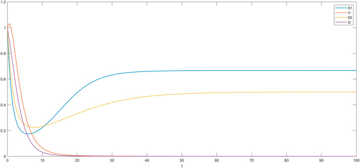
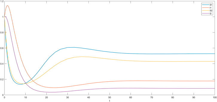
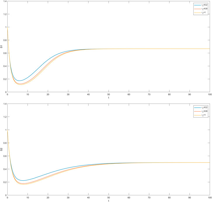
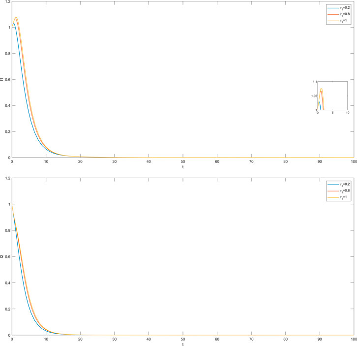
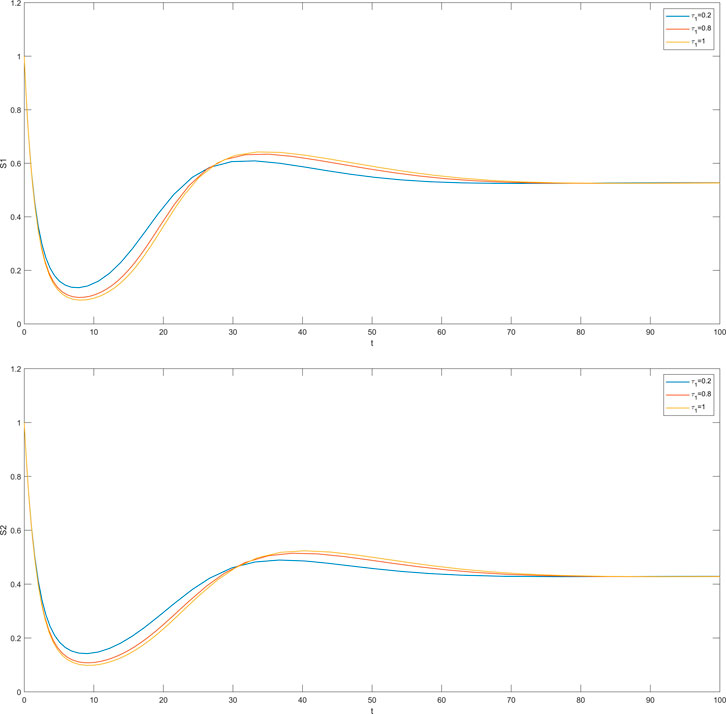
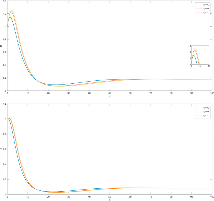
In this section, we simulate the influence of different time delays on susceptible and infected individuals in the impatient group and the level-headed group. The time delay
The cases where
The cases where
We consider that the intensity of the government measures can achieve the purpose of controlling the panic. The spread of panic is mainly dependent on the infected individuals. Therefore, Figure 7 indicates the comparison of trends of infected individuals in the two groups with and without control. On the one hand, a dramatic decrease in the trend of infected individuals with measures was derived. On the other hand, the time needed for the system to reach a steady state was reduced with measures. It can be seen that the control measures play an important role in the spread of panic and can effectively control the spread of panic.
6 Conclusion
In this study, the groups are divided into the impatient group and the level-headed group based on the psychological theory. Second, the susceptible individuals of the two groups are described by a single-species growth model. Third, a time-delayed panic-spreading model is established considering the influence of time delays for panic on the emotion transmission mechanism. The basic reproduction number of this model is calculated, and the conditions for the local and global asymptotic stability of the panic-free equilibrium and panic-permanent equilibrium are analyzed. To restrain the spread of emotions in emergencies, the government needs to take relevant measures, and the intensity of the measures taken is used to structure the optimal control model and minimize the control spread scale for emergencies. Finally, the related conclusions are illustrated by numerical simulations.
The aim of this study is to develop a model for simulating the spread process of panic. The results of the study are consistent with the trend of emotions in real situations. In the future, we will compare the results with those in other literature. Meanwhile, we simulate panic spreading in groups from a macroscopic perspective. Emotion spreading is a complex system from a microscopic perspective, considering the relationship between individuals and the external environment, and the rules of emotion spreading and interaction between individuals are also to be studied. Therefore, it is worth exploring emotion spreading in groups.
Data availability statement
The original contributions presented in the study are included in the article/Supplementary Material; further inquiries can be directed to the corresponding author.
Author contributions
Conceptualization: RL, HL, and QS. Data curation: RL. Formal analysis: RL. Funding acquisition: HL and QS. Investigation: RL. Methodology: RL. Project administration: HL and QS. Resources: HL and QS. Software: RL. Supervision: HL and QS. Validation: RL, HL, and QS. Visualization: RL. Writing—original draft: RL. Writing—review and editing: RL, HL, QS, and BL.
Funding
This research was funded by the Natural Science Foundation of China (71771112) and the Project of Liaoning Provincial Federation Social Science Circles of China (L20BGL047).
Conflict of interest
The authors declare that the research was conducted in the absence of any commercial or financial relationships that could be construed as a potential conflict of interest.
Publisher’s note
All claims expressed in this article are solely those of the authors and do not necessarily represent those of their affiliated organizations, or those of the publisher, the editors, and the reviewers. Any product that may be evaluated in this article, or claim that may be made by its manufacturer, is not guaranteed or endorsed by the publisher.
References
1. Fu L, Song W, Lv W, Lo S. Simulation of emotional contagion using modified SIR model: A cellular automaton approach. Physica A: Stat Mech its Appl (2014) 405:380–91. doi:10.1016/j.physa.2014.03.043
2. Adam C, Gaudou B, Taillandier P. Simulation of emotion dynamics in a group of agents in an evacuation situations. Berlin, Germany: Springer-Verlag (2010). p. 604–19. doi:10.1007/978-3-642-25920-3_44
3. Zheng L, Peng X, Wang L, Sun D. Simulation of pedestrian evacuation considering emergency spread and pedestrian panic. Physica A: Stat Mech its Appl (2019) 522:167–81. doi:10.1016/j.physa.2019.01.128
4. Mao Y, Du X, Li Y, He W. An emotion based simulation framework for complex evacuation scenarios. Graphical Models (2019) 102:1–9. doi:10.1016/j.gmod.2019.01.001
5. Helbing D, Farkas I, Vicsek T. Simulating dynamical features of escape panic. Nature (2000) 407(6803):487–90. doi:10.1038/35035023
6. Li R, Li Y, Meng Z, Song Y, Jiang G. Rumor spreading model considering individual activity and refutation mechanism simultaneously. IEEE Access (2000) 8(99):63065–76. doi:10.1109/ACCESS.2020.2983249
7. Xia Y, Jiang H, Yu Z. Global dynamics of ILSR rumor spreading model with general nonlinear spreading rate in multi-lingual environment. Chaos, Solitons & Fractals (2022) 154:111698. doi:10.1016/j.chaos.2021.111698
8. Jing W, Li Y, Zhang X, Zhang J, Jin Z. A rumor spreading pairwise model on weighted networks. Physica A: Stat Mech its Appl (2022) 585:126451. doi:10.1016/j.physa.2021.126451
9. Zheng T, Nie LF, Teng Z, Luo Y. Modeling seasonal variation for mosquito-borne disease in the tropical monsoon environment. Adv Differ Equ (2020) 1:469–16. doi:10.1186/s13662-020-02807-6
10. Sba B, Jg A, Fjc A, Sokolov IM, Lentz HH. Locally temperature - driven mathematical model of West Nile virus spread in Germany. J Theor Biol (2020) 488:110117. doi:10.1016/j.jtbi.2019.110117
11. Tian Z, Zhang G, Hu C, Lu D, Liu H. Knowledge and emotion dual-driven method for crowd evacuation. Knowledge-Based Syst (2020) 208(11):106451. doi:10.1016/j.knosys.2020.106451
12. Yin F, Xia X, Pan Y, She Y, Feng X, Wu J. Sentiment mutation and negative emotion contagion dynamics in social media: A case study on the Chinese sina microblog. Inf Sci (2022) 594:118–35. doi:10.1016/j.ins.2022.02.029
13. Hu Y, Pan Q, Hou W, He M. Rumor spreading model considering the proportion of wisemen in the crowd. Physica A: Stat Mech its Appl (2018) 505:1084–94. doi:10.1016/j.physa.2018.04.056
14. Jiang M, Gao Q, Zhuang J. Reciprocal spreading and debunking processes of online misinformation: A new rumor spreading–debunking model with a case study. Physica A: Stat Mech its Appl (2021) 565:125572. doi:10.1016/j.physa.2020.125572
15. Liu S, Ruan S, Zhang X. Nonlinear dynamics of avian influenza epidemic models. Math Biosciences (2017) 283:118–35. doi:10.1016/j.mbs.2016.11.014
16. Chen Y, Zhu S, He H. The influence of investor emotion on the stock market: Evidence from an infectious disease model. Discrete Dyn Nat Soc (2021) 9:1–12. doi:10.1155/2021/5520276
17. Zhao D, Li L, Peng H, Luo Q, Yang Y. Multiple routes transmitted epidemics on multiplex networks. Phys Lett A (2014) 378(10):770–6. doi:10.1016/j.physleta.2014.01.014
18. Zhao D, Wang L, Wang Z, Xiao G. Virus propagation and patch distribution in multiplex networks: Modeling, analysis, and optimal allocation. IEEE Trans Inform Forensic Secur (2019) 7(14):1755–67. doi:10.1109/TIFS.2018.2885254
19. Guo H, Yin Q, Xia C, Dehmer M. Impact of information diffusion on epidemic spreading in partially mapping two-layered time-varying networks. Nonlinear Dyn (2021) 105(4):3819–33. doi:10.1007/s11071-021-06784-7
20. Kang H, Fu C, Sun Z. Global exponential stability of periodic solutions for impulsive Cohen–Grossberg neural networks with delays. Appl Math Model (2015) 39(5–6):1526–35. doi:10.1016/j.apm.2014.09.015
21. Zhu L, Zhao H. Dynamical analysis and optimal control for a malware propagation model in an information network. Neurocomputing (2015) 149:1370–86. doi:10.1016/j.neucom.2014.08.060
22. Huo L, Ma C. The interaction evolution model of mass incidents with delay in a social network. Physica A: Stat Mech its Appl (2017) 484:440–52. doi:10.1016/j.physa.2017.04.162
23. Li L, Fu J, Zhang Y, Chai T, Song L, Albertos P. Output regulation for networked switched systems with alternate event-triggered control under transmission delays and packet losses. Automatica (2021) 131:109716. doi:10.1016/j.automatica.2021.109716
24. Li J, Jin Z, Sun G. Periodic solutions of a spatiotemporal predator-prey system with additional food. Chaos, Solitons & Fractals (2016) 91:350–9. doi:10.1016/j.chaos.2016.06.010
25. Adak D, Bairagi N, Hakl R. Chaos in delay-induced Leslie–Gower prey–predator–parasite model and its control through prey harvesting – ScienceDirect. Nonlinear Anal Real World Appl (2020) 2020:102998. doi:10.1016/j.nonrwa.2019.102998
26. Yu D, Wang G, Ding Q, Li T, Jia Y. Effects of bounded noise and time delay on signal transmission in excitable neural networks. Chaos, Solitons & Fractals (2022) 157:111929. doi:10.1016/j.chaos.2022.111929
27. Zheng T, Nie LF, Teng Z, Luo Y. Competitive exclusion in a multi-strain malaria transmission model with incubation period. Chaos, Solitons & Fractals (2020) 2020:109545. doi:10.1016/j.chaos.2019.109545
28. Wu W, Teng Z. Traveling waves in nonlocal dispersal SIR epidemic model with nonlinear incidence and distributed latent delay. Adv Differ Equ (2020) 1:614–26. doi:10.1186/s13662-020-03073-2
29. Khan A, Ikram R, Din A, Humphries UW, Akgul A. Stochastic COVID-19 SEIQ epidemic model with time-delay. Results Phys (2021) 30:104775. doi:10.1016/j.rinp.2021.104775
30. Rihan FA, Alsakaji HJ. Dynamics of a stochastic delay differential model for COVID-19 infection with asymptomatic infected and interacting people: Case study in the UAE. Results Phys (2021) 28:104658. doi:10.1016/j.rinp.2021.104658
31. Xia C, Wang Z, Sanz J, Meloni S, Moreno Y. Effects of delayed recovery and nonuniform transmission on the spreading of diseases in complex networks. Physica A: Stat Mech its Appl (2013) 392(7):1577–85. doi:10.1016/j.physa.2012.11.043
32. Cheng Y, Huo L, Zhao L. Dynamical behaviors and control measures of rumor-spreading model in consideration of the infected media and time delay. Inf Sci (2021) 564(3):237–53. doi:10.1016/j.ins.2021.02.047
33. Zhang J, Wang X, Xie Y, Wang M. Research on multi-topic network public opinion propagation model with time delay in emergencies. Physica A: Stat Mech its Appl (2022) 600:127409. doi:10.1016/j.physa.2022.127409
34. Hu J, Zhu L. Turing pattern analysis of a reaction-diffusion rumor propagation system with time delay in both network and non-network environments. Chaos, Solitons & Fractals (2021) 153:111542. doi:10.1016/j.chaos.2021.111542
35. Bolzoni L, Bonacini E, Soresina C, Groppi M. Time-optimal control strategies in SIR epidemic models. Math Biosci (2017) 292:86–96. doi:10.1016/j.mbs.2017.07.011
36. Grandits P, Kovacevic RM, Veliov VM. Optimal control and the value of information for a stochastic epidemiological SIS-model. J Math Anal Appl (2019) 476:665–95. doi:10.1016/j.jmaa.2019.04.005
37. Dai F, Liu B. Optimal control problem for a general reaction-diffusion eco-epidemiological model with disease in prey. Appl Math Model (2020) 88:1–20. doi:10.1016/j.apm.2020.06.040
38. Kang T, Zhang Q, Rong L. A delayed avian influenza model with avian slaughter: Stability analysis and optimal control. Physica A: Stat Mech its Appl (2019) 529:121544. doi:10.1016/j.physa.2019.121544
39. Bashier EBM, Patidar KC. Optimal control of an epidemiological model with multiple time delays. Appl Maths Comput (2017) 292:47–56. doi:10.1016/j.amc.2016.07.009
40. Wu D, Bai Y, Yu C. A new computational approach for optimal control problems with multiple time-delay. Automatica (2019) 101:388–95. doi:10.1016/j.automatica.2018.12.036
41. Sun G, Zhang H, Chang L, Jin Z, Wang H, Ruan S. On the dynamics of a diffusive foot-and-mouth disease model with nonlocal infections. SIAM J Appl Math (2022) 82:1587–610. doi:10.1137/21M1412992
42. Kouidere A, Kada D, Balatif O, Rachik M, Naim M. Optimal control approach of a mathematical modeling with multiple delays of the negative impact of delays in applying preventive precautions against the spread of the COVID-19 pandemic with a case study of Brazil and cost-effectiveness. Chaos, Solitons & Fractals (2021) 2021:110438. doi:10.1016/j.chaos.2020.110438
43. Ma X, Luo X, Li L, Li Y, Sun GQ. The influence of mask use on the spread of COVID-19 during pandemic in New York City. Results Phys (2022) 34:105224. doi:10.1016/j.rinp.2022.105224
44. Yusra BR, Maheshsingh M, Abdel AHK, Oree V, Dauhoo MZ. Assessing the impact of contact tracing, quarantine and red zone on the dynamical evolution of the covid-19 pandemic using the cellular automata approach and the resulting mean field system: A case study in Mauritius. Appl Math Model (2022) 11:567–89. doi:10.1016/j.apm.2022.07.008
45. Jkkaa B, Eo C, Aa D, Moore SE, Sun GQ, Jin Z, et al. Optimal control and comprehensive cost-effectiveness analysis for COVID-19. Results Phys (2022) 33:105177. doi:10.1016/j.rinp.2022.105177
46. Mathide M, Raluca E, Antoine P, Saussereau B. A multi-strain epidemic model for COVID-19 with infected and asymptomatic cases: Application to French data. J Theor Biol (2022) 545:111117. doi:10.1016/j.jtbi.2022.111117
47. Cao M, Zhang G, Wang M, Lu D, Liu H. A method of emotion contagion for crowd evacuation. Physica A: Stat Mech its Appl (2017) 483:250–8. doi:10.1016/j.physa.2017.04.137
48. Crescenzo AD, Paraggio P, Román-Román P, Torres-Ruiz F. Applications of the multi-sigmoidal deterministic and stochastic logistic models for plant dynamics. Appl Math Model (2020) 92:884–904. doi:10.1016/j.apm.2020.11.046
49. Dreessche P, Watmough J. Reproduction numbers and sub-threshold endemic equilibria for compartmental models of disease transmission. Math Biosci (2002) 180(1-2):29–48. doi:10.1016/S0025-5564(02)00108-6
50. Heffernan JM, Smith RJ, Wahl LM. Perspectives on the basic reproductive ratio. J R Soc Interf (2005) 2(4):281–93. doi:10.1098/rsif.2005.0042
Keywords: panic spreading, time-delay, stability analysis, optimal control, numerical simulation
Citation: Lv R, Li H, Sun Q and Li B (2022) Stability analysis and optimal control of a time-delayed panic-spreading model. Front. Phys. 10:1002512. doi: 10.3389/fphy.2022.1002512
Received: 26 July 2022; Accepted: 28 September 2022;
Published: 18 October 2022.
Edited by:
Gaogao Dong, Jiangsu University, ChinaCopyright © 2022 Lv, Li, Sun and Li. This is an open-access article distributed under the terms of the Creative Commons Attribution License (CC BY). The use, distribution or reproduction in other forums is permitted, provided the original author(s) and the copyright owner(s) are credited and that the original publication in this journal is cited, in accordance with accepted academic practice. No use, distribution or reproduction is permitted which does not comply with these terms.
*Correspondence: Hua Li, bGgxQHVzdGwuZWR1LmNu
 Rongjian Lv1
 Hua Li