 Shucheng Huang
 Junhui Yin
 Li Xu1,2
- 1National Key Laboratory of Science and Technology on Vacuum Electronics, School of Electronic Science and Engineering, University of Electronic Science and Technology of China, Chengdu, China
- 2Shenzhen Institute for Advanced Study, University of Electronic Science and Technology of China, Shenzhen, China
Over the last decades, the discontinuous Galerkin (DG) method has demonstrated its excellence in accurate, higher-order numerical simulations for a wide range of applications in aerodynamics simulations. However, the development of practical, computationally accurate flow solvers for industrial applications is still in the focus of active research, and applicable boundary conditions and fluxes are also very important parts. Based on curvilinear DG method, we have developed a flow solver that can be used for solving the three-dimensional subsonic, transonic and hypersonic inviscid flows on unstructured meshes. The development covers the geometrical transformation from the real curved element to the rectilinear reference element with the hierarchical basis functions and their gradient operation in reference coordinates up to full third order. The implementation of solid wall boundary conditions is derived by the contravariant velocities, and an enhanced algorithms of Harten-Lax-van Leer with contact (HLLC) flux based on curved element is suggested. These new techniques do not require a complex geometric boundary information and are easy to implement. The simulation of subsonic, transonic and hypersonic flows shows that the linear treatment can limit the accuracy at high order and demonstrates how the boundary treatment involving curved element overcomes this restriction. In addition, such a flow solver is stable on a reasonably coarse meshes and finer ones, and has good robustness for three-dimensional flows with various geometries and velocities. For engineering practice, a reasonable accuracy can be obtained at reasonably coarse unstructured meshes.
1 Introduction
Computational Fluid Dynamics (CFD) has become a very important and useful design tool in aerodynamics [1, 2]. The theoretical basis of CFD includes fluid mechanics, numerical analysis, computer technology and other fields. Based on the various calculation method [3–8], the approximate solution of the fluid governing equation is obtained by using the powerful computing capability of computer. In the past decades, due to the increasing demand for complex fluid flow simulations, great effort has been done by the CFD community in order to increase the accuracy and reduce the calculation costs [9–15]. It is now well understood that numerical errors play a key role in the accuracy of CFD results [10, 12]. In recent years, there has been an increasing interest in the application of high-order discretization methods with curved meshes, which can reduce the numerical errors to aerodynamic flows [16]. Curved meshes are commonly employed to provide a satisfactory representation of the domain boundary with only a moderate number of mesh elements, so that the polynomial degree can be increased while keeping the global number of degrees of freedom (DOFs). The role that curved meshes play in obtaining accurate solutions when combined with high-order numerical discretization methods has been demonstrated, such as [16–20]. Therefore, numerical discretization methods with curved meshes supporting arbitrary approximation orders have received an increasing amount of attention.
Initially developed for advection problems, the discontinuous Galerkin (DG) method has recently been applied in the field of CFD with great success [21–24]. The DG method combine two advantageous features commonly associated with finite element and finite volume methods [25]. As in classical finite element methods, accuracy is obtained by means of high-order polynomial approximation within an element rather than by wide stencils as in the case of finite volume methods. Conservation is, similarly to finite volume methods, enforced through the use of a flux at element boundaries, where a Riemann problem is solved [17]. Furthermore, the discretization lends itself to local mesh adaptation and efficient parallelization on modern distributed memory computer architectures. The implementation of efficient DG method on curved meshes is an open field of research and crucial for developing accurate numerical schemes. In the framework of the steady-state compressible inviscid flow, the necessity of a higher-order treatment of curved wall boundaries was put in evidence by Bassy and Rebay, and is now generally accepted [26, 27]. The curved meshes method via an isoparametric parametric approximation to curve boundary is rather convenient to use for DG schemes [22, 26]. A low-storage curvilinear DG method was proposed and analyzed in [28], where the geometric factors were included in both solution and test function spaces with a provable convergence under a mild condition on the mesh. Recent works by Chan et al. [29, 30] rely on reference frame polynomial spaces introducing weight-adjusted L2-inner products in order to recover high-order accuracy. In [20], a simple boundary treatment, which can be implemented as a modified DG scheme defined on triangles adjacent to boundary, was proposed. Even though integration along the curve is still necessary, integrals over any curved element are avoided. Blended isogeometric DG method formulated on elements that exactly preserve the CAD geometry have also been recently proposed in [31].
However, three-dimensional flows with curved meshes are rarely studied and the way to impose solid wall boundary conditions in curved meshes is not mentioned. Proper boundary treatment is critical in CFD. Its importance is obvious because it is the boundary conditions that determine the flow characteristics once the governing equations are given, at least for steady flow problems [32]. Even though the boundary conditions via a correct representation of the normal to the geometry is rather convenient to use for DG schemes [17, 27], the acquisition of normal is not very easy and needs to provide geometric information, which is not provided by the general mesh generator, especially when the boundary geometry is three-dimensional. Therefore, it is difficult to extend this curved meshes method to engineering applications. A highly adaptable numerical flux format is needed in aerodynamic simulations to accommodate a wide variety of flow velocities, including subsonic flow, transonic flow, supersonic flow and hypersonic flow, and so on. However, the implementation of numerical fluxes generally depends on Lax-Friedrichs scheme and Roe flux in the curved meshes. Although there are references to other (Godunov flux) format numerical fluxes, but display expression is not given. The Harten-Lax-van Leer with contact (HLLC) has gathered interest because of their accuracy, mathematical simplicity, inherent entropy satisfying property, positivity, lack of demand for knowledge of complete eigenstructure of flux Jacobians, ability to satisfactorily handle shocks and expansion fans and their easy extensibility to various hyperbolic systems of governing equations [33–35]. The HLLC scheme is one of the simplest known Riemann solver that can resolve both linearly degenerate and genuinely nonlinear wavefields accurately. Therefore, it is very significant for researchers to find a display expression for HLLC flux on curved meshes.
In recent years, open source solvers have also become very popular. Such as famous open source libraries libMesh [36] and deal.II [37]are both excellent, which have brought inspiration and convenience to many researchers. However, Local Lax-Friedrichs (LLF) flux was used in deal.II [37, 38]. LLF has a larger numerical viscosity, which is not as applicable as HLLC in practical engineering such as supersonic and transonic. In [39], Qiu also point out that the HLLC fluxes might be good choices as fluxes for the RKDG method when all factors such as the cost of CPU time, numerical errors and resolution of discontinuities in the solution are considered. The libMesh is more of a software framework than a complete solver. In practical problems, libMesh has almost no complete functional modules that can be directly applied, and researchers need to do secondary development according to the specific problems. Therefore, the development of three-dimensional solver of aerodynamics simulation is very meaningful work.
In the present work, for aerodynamics simulation, a simulation tool based on curvilinear DG method will be provided to include both three-dimensional solid walls boundary conditions on curved meshes and HLLC flux on curved meshes. First, we present the relevant closed form expressions for a widely used set of hierarchical basis functions up to full high order for a reference element, as well as the necessary expressions for the Jacobian for a high order polynomial geometrical transformation. Given these results, implementation is then straightforward. The derived expressions are used to implement the curved meshes, which are then applied to integration along curved element and curved face for complex geometries. Second, we present the implementation process of HLLC flux in the curved element. Third, the implementation of solid wall boundary conditions depends on contravariant velocities which include the Jacobian of the transformation function of the map from each curved element to a rectilinear reference element. Based on the above three points, we have developed a simulation tool that can be used for solving the three-dimensional subsonic, transonic and hypersonic inviscid flows. Academic problem of subsonic flow past a sphere is used to show how the linear treatment of wall boundaries limits the accuracy, and demonstrate how the boundary treatment involving curved element overcomes this restriction. The results suggest that such a scheme is stable on a reasonably coarse meshes and finer ones. Engineering problems of transonic flow past an ONERA M6 wing, hypersonic flow past a blunt cone, and hypersonic flow past a HB-2 ballistic model are used to demonstrate the ability of this method for engineering practice. Numerical tests suggest that the curvilinear DG method has great robustness for three-dimensional inviscid flows with various geometries and velocities on unstructured meshes.
The paper is organized as follows: we first discuss the main idea of curvilinear DG method in Section 2 for three-dimensional inviscid flows. We present an implementation process of HLLC flux with curved element in Section 3. As a demonstration, we discuss the boundary treatment in Section 4. Numerical tests are shown in Section 5. Section 6 consists of concluding remarks.
2 Discontinuous Galerkin discretization
2.1 Three-dimensional compressible Euler equations
The governing equations for the three-dimensional inviscid flow can be written as follows:
which is defined on a boundary domain
As is customary,
where
2.2 Discretization
The governing equation Eq. 1 is discretized using a DG finite element formulation which originally proposed in reference [40]. Here we provide a brief synopsis of the numerical scheme. For numerical discretization, we divide the problem domain
Then, approximate solution
where
where
Due to the discontinuous nature of the numerical solution, the normal flux
By assembling all the elemental contributions together, the system of ordinary differential equations which govern the evolution in time of the discrete solution can be written as
where
2.3 Geometric mapping of curved element
In order to improve the representation of curved wall boundaries, elements with second-order shape can be used in the vicinity of the geometry. The geometric transformation of the real curved element in
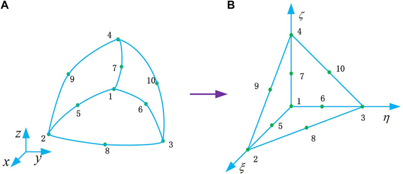
FIGURE 1. Curved element of global coordinates and rectilinear reference element of local coordinates, (A) is curved element, (B) is rectilinear reference element.
The transformation from reference to real coordinates is then accomplished by
where
In order to define and manipulate vector quantities within a curved element, the unitary base vectors (co-variant) are introduced
and the reciprocal base vectors are
Then, a vector can be represented by both its covariant components and the reciprocal base vectors
Differentiation in the reference coordinate system is connected to that in the real coordinate system as follows [22, 41]:
where
Then, Eq. 14 can be written as
where
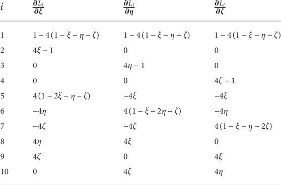
TABLE 1. Functions required for the Jacobian: second order curved element.
Although the expression is given, it is worth pointing out that the Jacobian is position-dependent within the element, and must be computed at each quadrature point when computing the integral of the volume and surface in the next subsection. It should be noted that the second order polynomial geometric transformation used here does not exactly model curved. More accurate geometrical modeling can be obtained by either increasing the order of the polynomial mapping or using tetrahedral rational Bezier volumes as shown in [43]. Although there are still some geometrical approximation errors, the fit is far better than that achieved using rectilinear elements.
2.4 Gradient operation of basis functions in reference coordinates
The basis functions and their gradient operation are derived for the parent element in terms of simplex coordinates. The actual set of basis functions used is the hierarchical type [44]. The hierarchical basis functions mean that the low order basis functions are maintained as a subset of the next higher-order basis functions. In order to derive the gradient on the reference element, the following associations are again made:
In the reference coordinates,
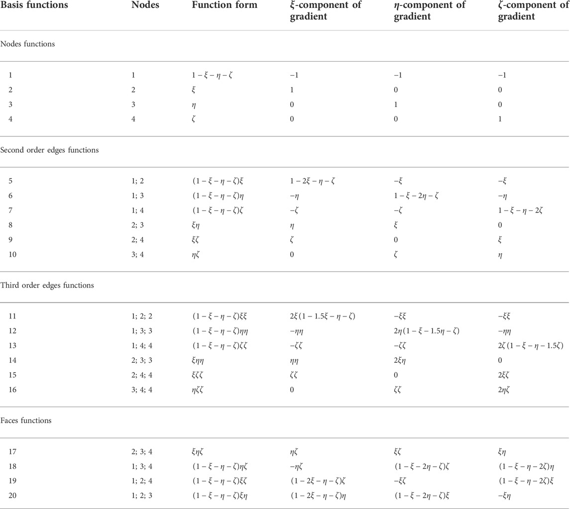
TABLE 2. Hierarchical basis functions and their gradient operation in reference coordinates.
2.5 Computation of integral of the volume and surface
The above subsections discussed geometric mapping of curved element. The real curved element (in the global
In Eq. 8, the mass matrix elements are computed as
and the residual vector elements are separated into the following two parts
where
In Eq. 22,
In the case where
in the case where
in the case where
and in the case where
where
The integral of the volume and surface cannot be evaluated analytically and must be computed numerically using quadrature techniques [45]. The use of high order quadrature rules results in increased computational cost when using curvilinear as opposed to rectilinear elements. Therefore, it is advisable that curved elements only be used along the curved boundaries of the domain.
3 The implementation process of Harten-Lax-van Leer with contact flux in curved element
Amongst various approximate Riemann solvers that exist in the literature, the HLLC schemes have gained popularity because of their simplicity and accuracy. In this work, we intend to closely study the numerical schemes of HLLC flux in curved element. The original Harten-Lax-van Leer (HLL) scheme was devised by Harten, Lax and van Leer [46]. It assumes a wave structure consisting of two waves that separates three constant states. Although quite accurate in resolution of nonlinear waves, a major drawback of the HLL scheme is its inability to exactly resolve the contact and shear waves. The loss of accuracy on these waves occurs because of the assumption of constant average state between the two wave structure [34]. The inability of HLL solver to resolve contact and shear waves was mitigated through the development of the HLLC Riemann solver (C for Contact) by Toro et al. [47]. This improvement was achieved by considering two averaged intermediate states, separated by adding a contact wave with speed
The two-state approximate Riemann solution is defined as [46]
The corresponding interface flux, denoted
where
In the rectilinear reference element, through Eq. 17, the unit normal vector
where
where
The choice of wavespeeds are given as [33]
where
Similarly, the jump relations across the
For three-dimensional Euler equations with states
Similarly, Eq. 35 becomes
To determine
where
where
Once
Multiplying the second, third, and fourth equations of Eq. 36 by
Using Eq. 41 this simplifies to give
With
From Eqs 41–47, the flux vector
4 Boundary conditions with curved element
4.1 Mesh generation
When exploiting the ability of higher-order discretization methods to generate accurate approximations on coarse meshes, a crucial point is to provide a proper representation of curved wall boundaries [23]. Using a finer mesh to fit the boundary is a common method. However, inserting additional elements close to a boundary with the sole purpose of resolving the geometry impedes the aims of higher-order methods.
A more adequate approach we pursue within the proposed method is to represent the boundary by Simmetrix’ Modeling Suite [49], which is able to cope with high-order meshes. We gain detailed information on the geometry via additional point data included in the mesh.
The curved mesh generation process is briefly illustrated by an example in Figure 2. Firstly, solver read the model and mesh parameters, then call the mesh generation module, and use a certain method (such as Delaunay triangulation) to generate the first-order meshes, as shown in Figures 2A,D. According to geometry information, second-order meshes are then produced by projecting the mid-point of boundary edges on the geometry, resulting in curved elements on the boundary, as shown in Figures 2B and Figure 2E.
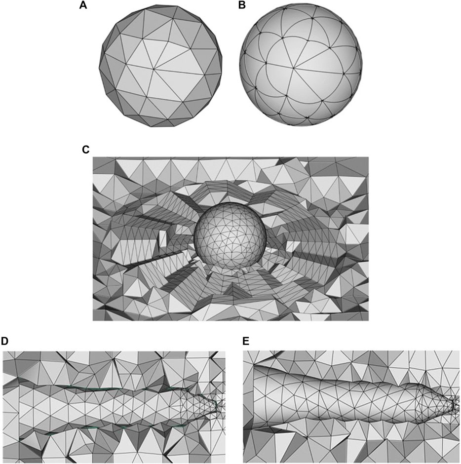
FIGURE 2. Detail of mesh generation process of sphere. (A) is first-order meshes of sphere, (B) is second-order meshes of sphere. (C) is computational domain meshes of sphere. (D) first-order meshes of HB-2, (E) second-order meshes of HB-2.
4.2 Boundary conditions
When the boundary face of an element belongs to
The reflecting boundary conditions state that no flow penetrates a solid wall, i.e., the normal velocity at the wall is zero. Depending on the numerical scheme, a ghost state or cell is created on the part of the numerical boundary
where
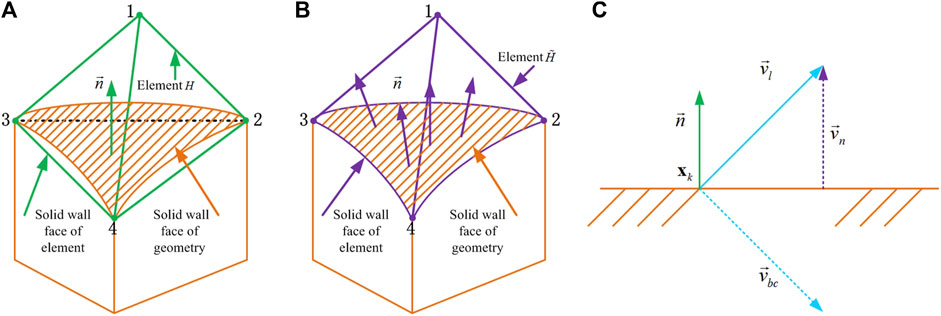
FIGURE 3. Solid wall boundary and geometric description of boundary conditions. (A) is rectilinear boundary element, (B) is curved boundary element, (C) is geometric description of boundary conditions.
A general process for implementing boundary conditions is shown below. A ghost state
where
while the density and pressure are copied exactly from the interior values at the same point. We obtain the ghost state vector as
Finally, the Riemann problem
This approach works well for straight-sided bodies. However, results are inferior when a physical geometry is more complex [27]. Even more, the DG method is highly sensitive to the error due to approximation of a curved geometry by a straight-sided element meshes. This error may dominate the discretization error of the scheme and lead to a wrong solution. We seek to impose boundary conditions which would take this into consideration and model flow more accurately. When considering the factors of the curved element, we proceed as follow.
In Section 4.1, we know that the solid wall boundary region is discretized by curved elements. When the boundary face of a curved element
Using the variables of rectilinear reference element, the normalized inward unit normal vector
where
where
From Eq. 49 we obtain the ghost state vector as
Since
5 Numerical examples
In order to demonstrate the performance of the proposed flow solver, we present several examples. All simulations were carried out on a Windows 10 64-bit Intel Core E5-2697 2.3-GHz and 256-GB RAM small workstation. For transonic flow and supersonic flow, the HWENO limiter in reference [50] is applied to the proposed flow solver. All computations were performed until solution coefficients reached a steady state, defined as the residual in reference [27].
5.1 Subsonic flow
We consider a subsonic flow at March number
First, we solve the problem on the sequence of meshes with
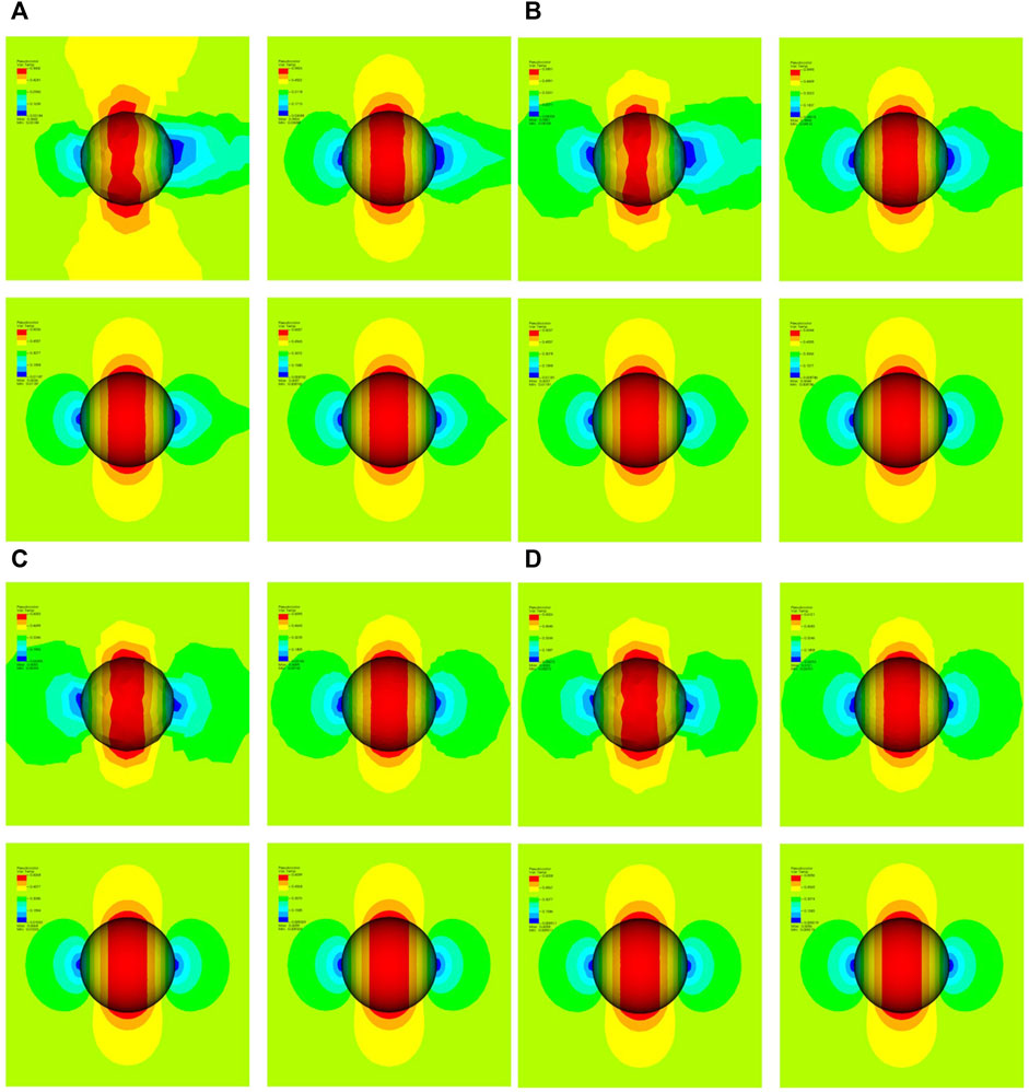
FIGURE 4. (A) Mach distribution with
The picture changes completely when using
To quantify our findings, we measure
where
where
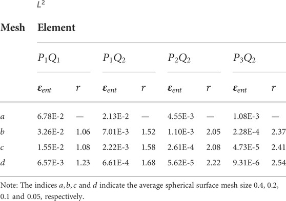
TABLE 3.
Further, we present two aerodynamic quantities: the pressure coefficient
and the total pressure loss coefficient defined as a ratio of the total pressure
at a point to the pressure of the free stream. The accuracy of the method is also evidenced by two aerodynamic quantities. The distribution of the pressure coefficient around the surface for four different meshes are shown in Figures 5A–D. The distribution of the total pressure loss coefficient around the surface for various meshes are shown in Figures 5E–H. We specify that mesh one to four refer to the coarse mesh to the fine mesh.
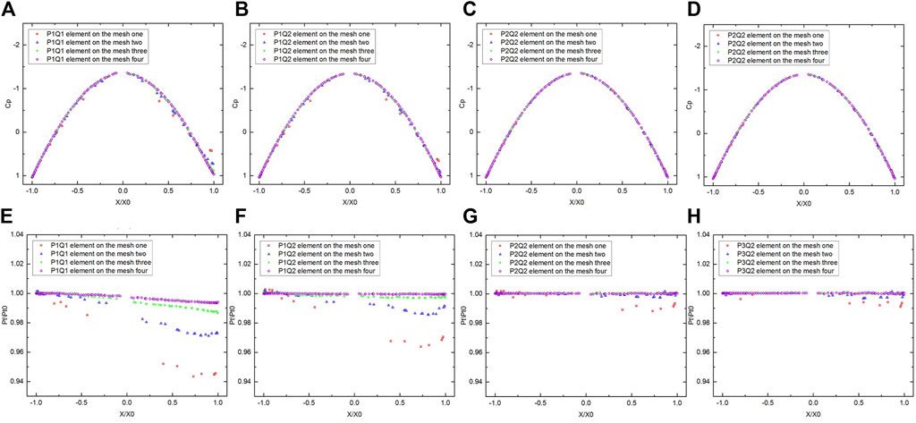
FIGURE 5. (A) Pressure coefficient distribution around a circle of sphere surface with
5.2 Transonic flow past ONERA M6 wing
A transonic flow over the ONERA M6 wing at a Mach number of
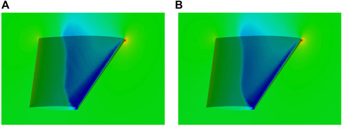
FIGURE 6. (A) The computed pressure distribution on the surface of ONERA M6 with
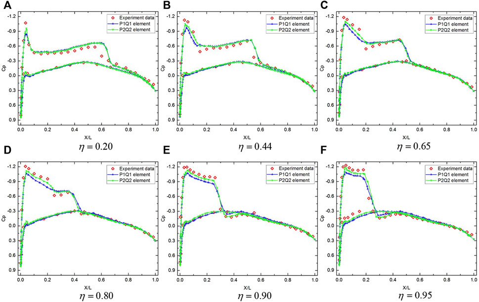
FIGURE 7. Comparison of the pressure coefficient distributions with experimental data for ONERA M6 wing at six span-wise locations. (A)
5.3 Hypersonic flow past blunt cone
This test case is selected to demonstrate that the proposed flow solver is able to solve hypersonic flow problems. The computation are performed for a high Mach number flow past the blunt cone model [53] using curvilinear and rectilinear DG method. The free stream Mach number, attack, pressure and temperature [53] for the blunt cone model correspond to
A three-dimensional axi-symmetric simulation is considered with the left and right boundaries defined as supersonic inflow and outflow boundaries respectively. The wall is modeled as a slip surface. The mesh used in this computation consists of 2,039,128 elements, 357,006 points. As with the previous definition,
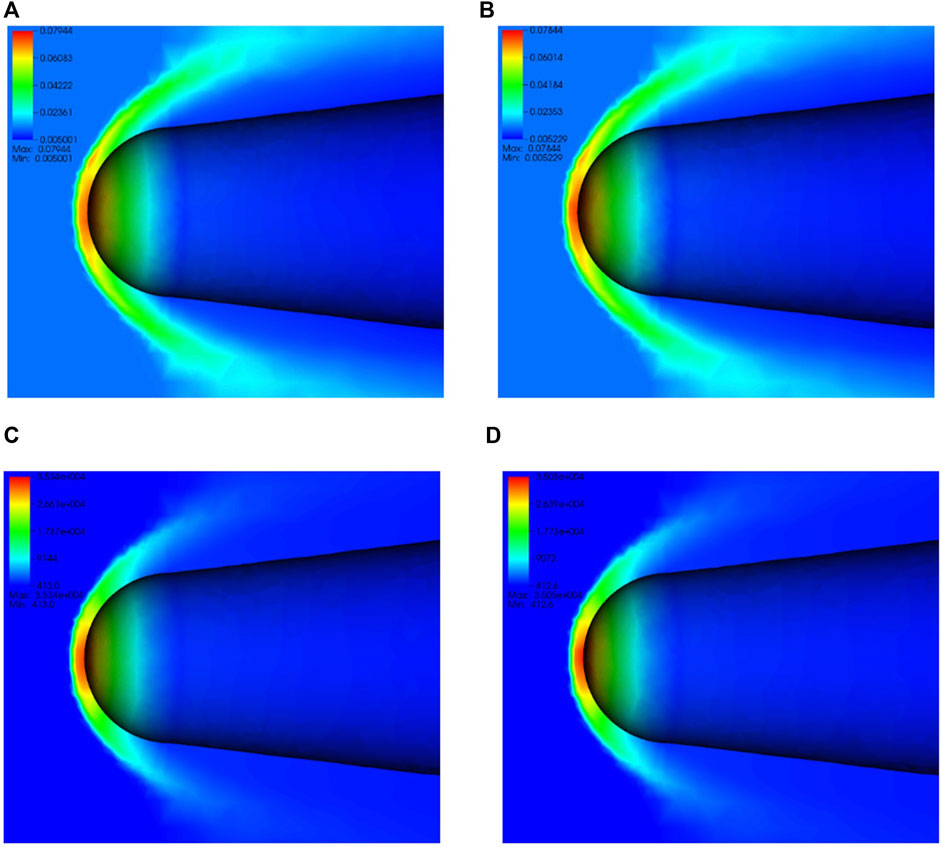
FIGURE 8. Computed flow distribution of (A) density with
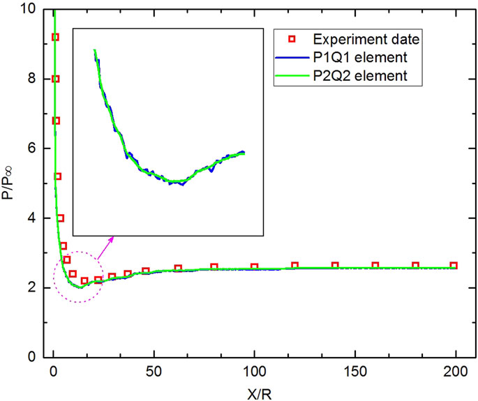
FIGURE 9. Comparison of the normalized pressure coefficient distributions with experimental data on the surface of blunt cone model.
5.4 Hypersonic flow past HB-2 ballistic model
Hypersonic flow past a HB-2 ballistic model is studied in this subsection. We carry out simulations at the flow conditions for which experimental setup details are available in the literature [54]. The free stream Mach number, attack, pressure and temperature [55, 56] for the HB-2 ballistic mode are
A three-dimensional axi-symmetric simulation is considered with the left and right boundaries defined as supersonic inflow and outflow boundaries respectively. The wall is modeled as a slip surface. The mesh used in this computation consists of 1,489,139 elements, 259,493 points. As with the previous definition,
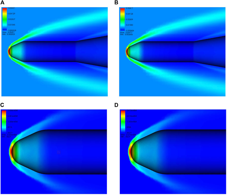
FIGURE 10. Computed flow distribution of (A) density with
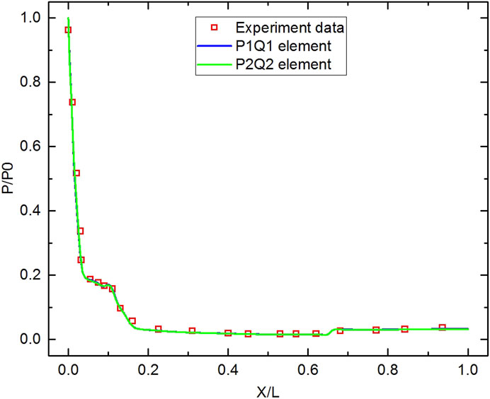
FIGURE 11. Comparison of the normalized pressure coefficient distributions with experimental data on the surface of HB-2 ballistic model.
6 Conclusion
A flow solver based on curvilinear DG method has been presented for solving the three-dimensional subsonic, transonic and hypersonic inviscid flows on curved meshes. The method aims to present the relevant closed form expressions for a widely used set of hierarchical basis functions up to full high order for a reference element, as well as the necessary expressions for the Jacobian for a high order polynomial geometrical transformation. Given these results, the implementation of solid walls boundary conditions is very simple because it is based on the contravariant velocities and does not require a complex geometric boundary information. Based on covariant vectors, an improved algorithm of HLLC flux for solving the subsonic, transonic and hypersonic flows is suggested. A number of numerical experiments for a variety of flow conditions have been conducted to demonstrate the superior performance of this flow solver (curvilinear) over the underlying method (rectilinear). The solution of subsonic flow past a sphere indicates that such a flow solver is stable on a reasonably coarse mesh and finer ones, and can get accurate results at reasonably coarse tetrahedral mesh. The solution of transonic flow past an ONERA M6 wing, hypersonic flow past a blunt cone and hypersonic flow past a HB-2 ballistic model verify that our flow solver has engineering practice value. The simulation of subsonic, transonic and hypersonic flows show that the flow solver has great robustness for three-dimensional fluids with various geometries and velocities. In future work, the developed method will be applied to more complicated geometries, and extended to viscosity flows with curve boundary layer.
Data availability statement
The original contributions presented in the study are included in the article/Supplementary Materials, further inquiries can be directed to the corresponding author.
Author contributions
SH: methodology and theoretical derivation, preprocess part and DGM coding, data curation and formal analysis, original draft writing and revising. JY: conceptualization, theoretical derivation, flux part coding, article review and editing, funding acquisition, project administration. LX: theoretical guidance, supervision and funding acquisition. BL: theoretical guidance, supervision. All authors discussed the results and contributed to manuscript revision. And all authors have read and agreed to the published version of the manuscript.
Funding
The author would like to acknowledge the financial support provided by the National Natural Science Foundation of China under Grant 12102087, 62071102, and 61921002.
Conflict of interest
The authors declare that the research was conducted in the absence of any commercial or financial relationships that could be construed as a potential conflict of interest.
Publisher’s note
All claims expressed in this article are solely those of the authors and do not necessarily represent those of their affiliated organizations, or those of the publisher, the editors and the reviewers. Any product that may be evaluated in this article, or claim that may be made by its manufacturer, is not guaranteed or endorsed by the publisher.
References
1. Oktay E, Alemdaroğlu N, Tarhan E, Champigny P, Espiney P. Unstructured euler solutions for missile aerodynamics. Aerosp Sci Technol (2000) 4(7):453–61. doi:10.1016/s1270-9638(00)01072-5
2. Pan J, Liu F. Wing flutter prediction by a small-disturbance euler method on body-fitted curvilinear grids. AIAA J (2019) 57(11):4873–84. doi:10.2514/1.j058120
3. Beghami W, Maayah B, Bushnaq S, Arqub OA. The laplace optimized decomposition method for solving systems of partial differential equations of fractional order. Int J Appl Comput Math (2022) 8(2):52–18. doi:10.1007/s40819-022-01256-x
4. Arqub OA, Hayat T, Alhodaly M. Analysis of lie symmetry, explicit series solutions, and conservation laws for the nonlinear time-fractional phi-four equation in two-dimensional space. Int J Appl Comput Math (2022) 8:145. doi:10.1007/s40819-022-01334-0
5. Srivastava HM, Iqbal J, Arif M, Khan A, Gasimov YS, Chinram R. A new application of gauss quadrature method for solving systems of nonlinear equations. Symmetry (2021) 13(3):432. doi:10.3390/sym13030432
6. Pourghanbar S, Manafian J, Ranjbar M, Aliyeva A, Gasimov YS. An efficient alternating direction explicit method for solving a nonlinear partial differential equation. Math Probl Eng (2020) 2020:1–12. doi:10.1155/2020/9647416
7. Arqub OA. Numerical simulation of time-fractional partial differential equations arising in fluid flows via reproducing kernel method. Int J Numer Methods Heat Fluid Flow (2019) 30:4711–33. doi:10.1108/hff-10-2017-0394
8. Arqub OA. Reproducing kernel algorithm for the analytical-numerical solutions of nonlinear systems of singular periodic boundary value problems. Math Probl Eng (2015) 2015:518406–13. doi:10.1155/2015/518406
9. Mascarenhas BS, Helenbrook BT, Atkins HL. Application of P-multigrid to discontinuous Galerkin formulations of the euler equations. AIAA J (2009) 47(5):1200–8. doi:10.2514/1.39765
10. Abbas A, Vicente JD, Valero E. Aerodynamic technologies to improve aircraft performance. Aerosp Sci Technol (2013) 28(1):100–32. doi:10.1016/j.ast.2012.10.008
11. Kouhi M, Onate E, Mavriplis D. Adjoint-based adaptive finite element method for the compressible euler equations using finite calculus. Aerosp Sci Technol (2015) 46:422–35. doi:10.1016/j.ast.2015.08.008
12. Ponsin J, Fraysse F, Gomez M, Cordero-Gracia M. An adjoint-truncation error based approach for goal-oriented mesh adaptation. Aerosp Sci Technol (2015) 41:229–40. doi:10.1016/j.ast.2014.10.021
13. Deng X, Xie B, Xiao F. Multimoment finite volume solver for euler equations on unstructured grids. AIAA J (2017) 55(8):2617–29. doi:10.2514/1.j055581
14. Pagliuca G, Timme S. Model reduction for flight Dynamics simulations using computational fluid Dynamics. Aerosp Sci Technol (2017) 69:15–26. doi:10.1016/j.ast.2017.06.013
15. Liu Y, Zhang W, Kou J. Mode multigrid-a novel convergence acceleration method. Aerosp Sci Technol (2019) 92:605–19. doi:10.1016/j.ast.2019.06.001
16. Botti L, Pietro DAD. Assessment of hybrid high-order methods on curved meshes and Comparison with discontinuous Galerkin methods. J Comput Phys (2018) 370:58–84. doi:10.1016/j.jcp.2018.05.017
17. Toulorge T, Desmet W. Curved boundary treatments for the discontinuous Galerkin method applied to aeroacoustic propagation. AIAA J (2010) 48(2):479–89. doi:10.2514/1.45353
18. Bassi F, Botti L, Colombo A, Rebay S. Agglomeration based discontinuous Galerkin discretization of the euler and Navier-Stokes equations. Comput Fluids (2012) 61:77–85. doi:10.1016/j.compfluid.2011.11.002
19. Zhang X, Tan S. A simple and accurate discontinuous Galerkin scheme for modeling scalar-wave propagation in media with curved interfaces. Geophysics (2015) 80(2):T83–T9. doi:10.1190/geo2014-0164.1
20. Zhang X. A curved boundary treatment for discontinuous Galerkin schemes solving time dependent problems. J Comput Phys (2016) 308:153–70. doi:10.1016/j.jcp.2015.12.036
21. Cockburn B, Karniadakis GE, Shu CW. Discontinuous Galerkin methods: Theory, computation and applications. New York: Springer Science & Business Media (2012).
22. Hesthaven JS, Warburton T. Nodal discontinuous Galerkin methods: Algorithms, analysis, and applications. New York: Springer Science & Business Media (2007).
23. Hartmann R, Held J, Leicht T, Prill F. Discontinuous Galerkin methods for computational aerodynamics-3d adaptive flow simulation with the dlr padge code. Aerosp Sci Technol (2010) 14(7):512–9. doi:10.1016/j.ast.2010.04.002
24. Antonietti PF, Cangiani A, Collis J, Dong Z, Georgoulis EH, Giani S, et al. Review of discontinuous Galerkin finite element methods for partial differential equations on complicated domains. Cham: Springe (2016).
25. Luo H, Xia Y, Spiegel S, Nourgaliev R, Jiang Z. A reconstructed discontinuous Galerkin method based on a hierarchical weno reconstruction for compressible flows on tetrahedral grids. J Comput Phys (2013) 236:477–92. doi:10.1016/j.jcp.2012.11.026
26. Bassi F, Rebay S. High-order accurate discontinuous finite element solution of the 2d euler equations. J Comput Phys (1997) 138(2):251–85. doi:10.1006/jcph.1997.5454
27. Krivodonova L, Berger M. High-order accurate implementation of solid wall boundary conditions in curved geometries. J Comput Phys (2006) 211(2):492–512. doi:10.1016/j.jcp.2005.05.029
28. Warburton T. A low-storage curvilinear discontinuous Galerkin method for wave problems. SIAM J Sci Comput (2013) 35(4):A1987–A2012. doi:10.1137/120899662
29. Chan J, Hewett RJ, Warburton T. Weight-adjusted discontinuous Galerkin methods: Curvilinear meshes. SIAM J Sci Comput (2017) 39(6):A2395–A421. doi:10.1137/16m1089198
30. Chan J, Wilcox LC. On discretely entropy stable weight-adjusted discontinuous Galerkin methods: Curvilinear meshes. J Comput Phys (2019) 378:366–93. doi:10.1016/j.jcp.2018.11.010
31. Michoski C, Chan J, Engvall L, Evans JA. Foundations of the blended isogeometric discontinuous Galerkin (bidg) method. Comput Methods Appl Mech Eng (2016) 305:658–81. doi:10.1016/j.cma.2016.02.015
32. Wang ZJ, Sun Y. Curvature-based wall boundary condition for the euler equations on unstructured grids. AIAA J (2003) 41(1):27–33. doi:10.2514/2.1931
33. Batten P, Clarke N, Lambert C, Causon DM. On the choice of wavespeeds for the hllc Riemann solver. SIAM J Sci Comput (1997) 18(6):1553–70. doi:10.1137/s1064827593260140
34. Simon S, Mandal JC. A cure for numerical shock instability in hllc Riemann solver using antidiffusion control. Comput Fluids (2018) 174:144–66. doi:10.1016/j.compfluid.2018.07.001
35. Simon S, Mandal JC. A simple cure for numerical shock instability in the hllc Riemann solver. J Comput Phys (2019) 378:477–96. doi:10.1016/j.jcp.2018.11.022
36. Kirk BS, Peterson JW, Stogner RH, Carey GF. Libmesh : A C++ library for parallel adaptive mesh refinement/coarsening simulations. Eng Comput (2006) 22(3-4):237–54. doi:10.1007/s00366-006-0049-3
37. Bangerth W. Deal.Ii (2021). Available from https://www.dealii.org/ (Accessed August 16, 2022).
38. Bangerth W. Deal.Ii the step-67 tutorial program (2021). Available from https://www.dealii.org/current/doxygen/deal.II/step_67.html (Accessed August 17, 2022).
39. Qiu J, Khoo B, Shu CW. A numerical study for the performance of the Runge-Kutta discontinuous Galerkin method based on different numerical fluxes. J Comput Phys (2006) 212(2):540–565. doi:10.1016/j.jcp.2005.07.011
40. Cockburn B, Shu CW. The Runge–Kutta discontinuous Galerkin method for conservation laws V: Multidimensional systems. J Comput Phys (1998) 141(2):199–224. doi:10.1006/jcph.1998.5892
41. Swartz JP, Davidson DB. Curvilinear vector finite elements using a set of hierarchical basis functions. IEEE Trans Antennas Propag (2007) 55(2):440–6. doi:10.1109/tap.2006.888448
42. Fahs H. Improving accuracy of high-order discontinuous Galerkin method for time-domain electromagnetics on curvilinear domains. Int J Comput Math (2011) 88(10):2124–53. doi:10.1080/00207160.2010.527960
43. Martini E, Pelosi G, Selleri S. A hybrid finite-element-modal-expansion method with a new type of curvilinear mapping for the analysis of microwave passive devices. IEEE Trans Microw Theor Tech (2003) 51(6):1712–7. doi:10.1109/tmtt.2003.812571
44. Yin JH, Xu L, Wang H, Xie P, Huang SC, Liu HX, et al. Accurate and fast three-dimensional free vibration analysis of large complex structures using the finite element method. Comput Struct (2019) 221:142–56. doi:10.1016/j.compstruc.2019.06.002
45. Zhang L, Cui T, Liu H. A set of symmetric quadrature rules on triangles and tetrahedra. J Comput Math (2009) 27(1):89–96.
46. Harten A, Lax PD, Leer BV. On upstream differencing and godunov-type schemes for hyperbolic conservation laws. SIAM Rev (1983) 25(1):35–61. doi:10.1137/1025002
47. Toro EF, Spruce M, Speares W. Restoration of the contact surface in the hll-riemann solver. Shock Waves (1994) 4(1):25–34. doi:10.1007/bf01414629
48. Roe PL. Approximate Riemann solvers, parameter vectors, and difference schemes. J Comput Phys (1981) 43(2):357–72. doi:10.1016/0021-9991(81)90128-5
49. Simmetrix I. Simmetrix’ modeling suite (2013). Available from http://www.simmetrix.com (Accessed August 6, 2021).
50. Luo H, Baum JD, Löhner R. A hermite weno-based limiter for discontinuous Galerkin method on unstructured grids. J Comput Phys (2007) 225(1):686–713. doi:10.1016/j.jcp.2006.12.017
51. Schmitt V, Charpin F. Pressure distributions on the Onera-M6-Wing at transonic mach numbers. Exp Data base Comput Program Assess. Report of the Fluid Dynamics Panel Working Group 04, AGARD AR 138 (1979). Available from http://www.ttctech.com/samples/onera_m6_wing_multiblock/onera_mb.htm.
52. Batina JT. Accuracy of an unstructured-grid upwind-euler algorithm for the onera M6 wing. J Aircr (1991) 28(6):397–402. doi:10.2514/3.46040
53. Zhong X, Ma Y. Boundary-layer receptivity of Mach 7.99 flow over a blunt cone to free-stream acoustic waves. J Fluid Mech (2006) 556:55–103. doi:10.1017/s0022112006009293
54. Damljanović D, Rašuo B, Đ V, Mandić S, Isaković J. Hypervelocity ballistic reference models as experimental supersonic test cases. Aerosp Sci Technol (2016) 52:189–97. doi:10.1016/j.ast.2016.02.035
55. Tissera S. Assessment of high-resolution methods in hypersonic real-gas flows. Cranfield: Cranfield University (2010).
Keywords: discontinuous Galerkin method, HLLC flux, curved element, high order accuracy, transonic flow simulation, hypersonic flow simulation
Citation: Huang S, Yin J, Xu L and Li B (2022) Aerodynamics simulations of three-dimensional inviscid flow using curvilinear discontinuous Galerkin method on unstructured meshes. Front. Phys. 10:1000635. doi: 10.3389/fphy.2022.1000635
Received: 22 July 2022; Accepted: 17 October 2022;
Published: 01 November 2022.
Edited by:
Alexander Kurganov, Southern University of Science and Technology, ChinaReviewed by:
Omar Abu Arqub, Al-Balqa Applied University, JordanYusif Gasimov, Azerbaijan University, Azerbaijan
Copyright © 2022 Huang, Yin, Xu and Li. This is an open-access article distributed under the terms of the Creative Commons Attribution License (CC BY). The use, distribution or reproduction in other forums is permitted, provided the original author(s) and the copyright owner(s) are credited and that the original publication in this journal is cited, in accordance with accepted academic practice. No use, distribution or reproduction is permitted which does not comply with these terms.
*Correspondence: Junhui Yin, eWluamhAdWVzdGMuZWR1LmNu