Exploring Optimality of Piecewise Polynomial Interpolation Functions for Lung Field Modeling in 2D Chest X-Ray Images

In this paper, a landmark based approach, using five different interpolating polynomials (linear, cubic convolution, cubic spline, PCHIP, and Makima) for modeling of lung field region in 2D chest X-ray images have been presented. Japanese Society of Radiological Technology (JSRT) database which is publicly available has been used for evaluation of the proposed method. Selected radiographs are anatomically landmarked using 17 and 16 anatomical landmark points to represent left and right lung field regions, respectively. Local, piecewise polynomial interpolation is then employed to create additional semilandmark points to form the lung contour. Jaccard similarity coefficients and Dice coefficients have been used to find accuracy of the modeled shape through comparison with the prepared ground truth. With the optimality condition of three intermediate semilandmark points, PCHIP interpolation method with an execution time of 5.04873 s is found to be the most promising candidate for lung field modeling with an average Dice coefficient (DC) of 98.20 and 98.54% (for the left and right lung field, respectively) and with the average Jaccard similarity coefficient (JSC) of 96.47 and 97.13% for these two lung field regions. While performance of Makima and cubic convolution is close to the PCHIP with the same optimality condition, i.e., three intermediate semilandmark points, the optimality condition for the cubic spline method is of at least seven intermediate semilandmark points which, however, does not result in better performance in terms of accuracy or execution time.

1 Introduction

The chest X-ray imaging is still one of the most preferred techniques that radiologists and medical practitioners use to diagnose the lung diseases in their daily routine checkups due to its low cost and easy availability. Due to this reason, the accurate detection and segmentation of the lung field region are of prime importance for any biomedical image analysis procedures [1–3]. Delineation of the lung field is a prerequisite for any chest-image analysis procedure. However, delineation is a very tedious and time-consuming procedure that may be prone to subjective bias. Therefore, an automated solution for the lung field segmentation is needed [4]. The development of an automated solution for the lung field segmentation is challenging due to intensity variations across the edges and overlapping of the other anatomical structures. As chest X-rays are low contrast images, the lung regions cannot be differentiated from the background and hence the classical approaches like thresholding and edge detection algorithms are not sufficient enough for the lung field segmentation. The author in Ref. [5] provided an intuitive method to solve this problem by representing a shape as a set of discrete labeled points and referred to these points as landmarks. Each labeled point represents a particular part of the shape or its boundary and captures certain distribution in the shape space. But in practice, it is very time-consuming. Labeling a set of landmark points to model a shape in the shape space is referred as point distribution model (PDM) [6,7]. The modeled shape takes a considerable amount of landmark points to form a curve. Thus, the point distribution model inevitably reduces the number of points that may use to represent a shape. Clearly, these labeled sets or the number of landmark points do not represent any salient feature of anatomical significance, but a part of the curve or boundary of the anatomical shape. However, this method (PDM) has some undesirable consequences. First, users are forced to put many landmark points to smooth out the curve in every training example. Second, the landmark points may lose their characteristics as true landmark point as they do not represent any salient feature of the object. The above said problem can be minimized by taking only a few landmark points that must characterize some anatomical significance of the lung field region. These significant anatomical landmark points are then interpolated to get a close approximation of the original lung field shape. The accurate delineation of the lung field requires the anatomical knowledge of chest radiography to incorporate the expected shape that may work as a priori information in active shape modeling (ASM).

To delineate the lung fields, the author in Ref. [8] used 50 landmark points for the left lung and 44 landmark points for the right lung representation. They also used 26 landmark points for the heart shape representation and a pair of 23 landmark points for the left and right clavicle’s (left and right) representation. Each object and landmark point was defined by manual annotation, and no interpolation method was employed. The author in Ref. [9] proposed a lung segmentation methodology by capturing salient points around the lung fields by subsequent application of simple intensity and edge feature extraction techniques. The detected salient points are then interpolated using Bezier curves to approximate the lung field boundaries. In Ref. [10], Shao et al. presented a joint shape and appearance sparse learning method to segment out lung field from the chest radiographs. They used a total of 14 labeled points (6 for the right lung and 8 for the left lung) to get a rough idea of both the lung regions. They termed these labeled sets as “landmarks.” Few more points were also annotated between these landmark points, and they termed these labeled sets as “points.” However, the authors did not provide any information about the number of points they used to represent the lung field regions. The author in Ref. [11] presented a customized active shape model to extract the lung regions from the chest X-ray images. They employed an average active shape model, gray scale projection, and affine registration to obtain the initial lung contours. After that, an objective function is defined to push the vertices of the active shape model to the real lung edges to get a more balanced distance distribution of vertices. They used 44 and 50 landmark points to represent the left and the right lung regions for the lung field segmentation. The annotated set of landmark points was manually defined and interpolation was not employed. The author in Ref. [12] presented an automatic lung field segmentation method using an improved statistical shape and appearance model. They used 6 landmark points to locate each lung region and then applied a gray-level intensity based method to locate and initialize the lung shape model. They used the intensity profile model to create boundary landmark points and later these landmark points were interpolated by a cubic spline interpolation method. In Ref. [13], the authors used the set of labeled points to train their algorithm for the automatic lung field segmentation using active shape modeling (ASM) in the single-photon emission computerized tomography (SPECT) images and validated this automatic SPECT segmentation against computed tomography (CT) images as well as manually delineated SPECT images. But the method does not explain the type of interpolation mechanism that they used. In Ref. [14], the authors used 144 annotated boundary points (72 per left/right lung) to construct a statistical shape model of the lung field. Specifically, they used six manually annotated primary landmark points based on the appearance of the lung field and then secondary landmarks were estimated along the lung contour using interpolation between the manually annotated primary landmarks. However, it is noted that the other anatomical structures that overlap with the lung field region were not excluded in their method, and the type of the interpolation method was not defined. All these authors used the landmark selection method to segment out lung field regions from the chest radiographic images. However, these authors could not explain the number of interpolating points (secondary landmarks) that is needed to approximate the lung field regions with the highest similarity index.

The landmarking method is also employed to delineate other anatomical structures like the heart, liver, femur, etc., in CT, SPECT, and other medical imaging techniques. The authors in Ref. [15] reported a general multi-resolution framework for the statistical modeling of multi-object structures. The authors in Ref. [16] proposed a dual active shape model for the segmentation of heart’s right ventricle (RV) boundary. The authors in Ref. [17] presented an automatic liver segmentation method using the shape modeling methods in computed tomography (CT) images. The authors in Ref. [18] used landmark based method for extracting prostate boundaries from the 2D transrectal ultrasound (TRUS) images by using a partial active shape model (PASM). The authors in Ref. [16] introduced an ASM-based framework for motion correction of myocardial T1 mapping in magnetic resonance imaging (MRI). Clearly, landmarking is the first stage of any automated computer aided diagnostic (CAD) system that tries to identify the anatomical region. The landmark based method’s major strength is that it represents a shape as a set of discrete labeled points. The landmark based method is highly applicable for the cases where the visibility of the boundary is obscured or cannot be differentiated from the background, which is always the case of low contrast imaging like X-ray and ultrasound imaging. The landmark based point distribution model finds numerous applications in active shape modeling (ASM), active appearance modeling, deep learning (DL), and machine learning (ML) models for the registration and segmentation applications in medical imaging. However, there are some limitations of this method that preclude their accurate clinical application. The model based methods assume that the shape information and intensity information between the training images and the new image to be segmented are similar to each other. Unfortunately, this assumption can often be invalid due to the variability of the lung’s anatomy among the individuals in the application stages.

In this paper, a set of landmark points based on the anatomical properties of the left lung region and right lung field regions are explored. Our contributions in this paper are 1) identification of the number of anatomical landmark points in the thorax region for the left and right lung field modeling, 2) identification of the optimality condition of each of the interpolating polynomial to model left and right lung field region, and 3) identification of the most suited interpolating polynomial that models the left and right lung field region with highest similarity index by producing least number of secondary landmark points. Exploring the optimality of piecewise polynomials has an added advantage over selecting a random number of semilandmark points. It minimizes the number of interpolating points and hence reduces the computational complexity of the processing algorithm. Knowing the minimum number of interpolating points is highly beneficial in real-time medical imaging applications requiring less computational complexity. However, one disadvantage of landmark based study is that the number of available landmark points can sometimes be insufficient to capture the shape of an object.

The remainder of this paper is organized as follows: Section 2 provides the mathematical foundation of the lung shape modeling and Section 3 discusses the interpolation methods that mainly highlight the different categories of piecewise cubic interpolating polynomial that we have used in this literature. Section 4 discusses the methods under which the images are landmarked, and, finally, Section 5 and Section 6 discuss the simulation results and conclusion, respectively.

2 Lung Shape Modeling

Let each shape in the training set be represented by a set of K number of landmark positions that must be consistent from one shape to the next. Here, the consistency employs that each particular landmark point must be placed on the same site as it was on the first image. That means, each particular landmark point represents a specific location of the lung field boundary.

To model a lung field shape, let each annotated landmark point be represented by the coordinate position (x_j, y_j) in the two dimensional space ${\mathbb{R}}^2$. If each shape is annotated by K number of landmark points, then the modeled shape in terms of coordinate positions for the ith shape is defined by [19]

$S_i=(x_{ij},y_{ij});wherej=[1\cdots K](1)$

These coordinate position $S_i=\left((x_{i1},y_{i1}),(x_{i2},y_{i2}),\dots ,(x_{ik},y_{ik})\right)$ in a shape vector form can be represented as

${\mathbf{S}}_{\mathrm{i}}=\left[{\mathbf{x}}_{\mathbf{i1}},{\mathbf{y}}_{\mathbf{i1}},{\mathbf{x}}_{\mathbf{i2}},{\mathbf{y}}_{\mathbf{i2}},\dots ,{\mathbf{x}}_{\mathbf{ik}},{\mathbf{y}}_{\mathbf{ik}}\right](2)$

that is further rearranged as a set of 2K vector:

${\mathbf{S}}_{\mathbf{i}}={\left[{\mathbf{x}}_{\mathbf{i1}},{\mathbf{x}}_{\mathbf{i2}},\dots ,{\mathbf{x}}_{\mathbf{ik}},{\mathbf{y}}_{\mathbf{i1}},{\mathbf{y}}_{\mathbf{i2}},\dots ,{\mathbf{y}}_{\mathbf{ik}}\right]}^{\mathbf{T}}(3)$

$or{\mathbf{S}}_{\mathbf{i}}={\left[{\mathbf{S}}_{\mathbf{ix}},{\mathbf{S}}_{\mathbf{iy}}\right]}^{\mathbf{T}}\in {\mathbb{R}}^{2K\times 1}(4)$

where

${\mathbf{S}}_{\mathbf{ix}}=[{\mathbf{x}}_{\mathbf{i1}},{\mathbf{x}}_{\mathbf{i2}},\dots ,{\mathbf{x}}_{\mathbf{ik}}]\in {\mathbb{R}}^{K\times 1}(5)$

${\mathbf{S}}_{\mathbf{iy}}=[{\mathbf{y}}_{\mathbf{i1}},{\mathbf{y}}_{\mathbf{i2}},\dots ,{\mathbf{y}}_{\mathbf{ik}}]\in {\mathbb{R}}^{K\times 1}(6)$

If there are L number of training examples, then the configuration matrix $S\in {\mathbb{R}}^{2K\times L}$ can be written as

$\mathbf{S}=[{\mathbf{S}}_{\mathbf{1}},{\mathbf{S}}_{\mathbf{2}},\dots ,{\mathbf{S}}_{\mathbf{L}}]\in {\mathbb{R}}^{2K\times L}(7)$

3 Interpolation Methods

Modeling or building a shape requires the function to be continuous. This creates a real problem if the modeling function consists of a set of discrete data points (landmark points). Therefore, it requires to construct a continuous function based on discrete data points. Here, an attempt is made to examine different interpolation techniques that fit the shape in a continuous manner from a set of discrete landmark points. Interpolation helps to construct a continuous function from a set of discrete data points. It is to be noted that, these interpolation techniques [20] only provide the conditions under which the lung field regions are modeled. The methods do not provide any solution to the explained techniques.

Given K number of landmark points (x_j, y_j) in the 2D-plane ${\mathbb{R}}^2$, the interpolating polynomial is defined as

$P(x_j)=y_j;j=(1,\dots ,k)(8)$

where x = (x₁, … , x_k) are the interpolation points and P(x_j) is the interpolating polynomial of the landmark point (x₁, y₁), (x₂, y₂), …, (x_k, y_k). Solving a fitting polynomial P(x_j) that fits the landmark point (x_j, y_j) is equivalent to solving a system of linear equation

${\mathbf{A}\mathbf{S}}_{\mathbf{ix}}={\mathbf{S}}_{\mathbf{iy}}(9)$

where A is a Vandermonde matrix.

3.1 Piecewise Polynomial Interpolation

A quite natural and different approach to approximate a function on an interval is to first split the interval into subintervals and then approximate the function by a polynomial of fairly low degree on each subinterval.

Given K number of landmark point $\left(x_j,y_j\right)\in {\mathbb{R}}^2$ with the condition x₁ < x₂ < ⋯ < x_k, the one dimensional piecewise interpolant in terms of piecewise function can be defined as

$P(x)=P_j(x),x\in \left[x_j,x_{j+1}\right](10)$

where P_j(x) is at least continuous everywhere in $\left[x_j,x_{j+1}\right]$. Continuity condition should hold at every data point,

$P_j(x_{j+1})=P_{j+1}(x_{j+1})(11)$

A piecewise polynomial function is defined as

$P_j(x)=\sum _{r=1}^k{a}_r^j{\left(x-x_j\right)}^r(12)$

Hence, the piecewise polynomial interpolation problem is to determine the coefficients $a_r^j$ for all of the intervals such that the resulting interpolant has desirable properties.

3.2 Linear Interpolation

Piecewise linear interpolation [21] is by far the most popular interpolation technique that finds numeral application in signal and image processing due to its faster performance.

If t is the local variable given by t = x − x_j, $x\in \left[x_j,x_{j+1}\right]$, then the divided difference δ_j is

${\delta }_j=\frac{y_{j+1}-y_j}{x_{j+1}-x_j};j=1\cdots (k-1)(13)$

The piecewise linear interpolation is then piecewise straight lines connecting two consecutive points of the interval $\left(x_j,x_{j+1}\right)$. The interpolant in the interval $\left(x_j,x_{j+1}\right)$ is then

$P(x)=y_j+\left(x-x_j\right)\frac{y_{j+1}-y_j}{x_{j+1}-x_j}(14)$

or

$P(x)=y_j+t{\delta }_j(15)$

clearly, this equation represents a function of straight line that passes through the landmark positions $\left(x_j,y_j\right)$ and $\left(x_{j+1},y_{j+1}\right)$.

3.3 Cubic Convolution Interpolation

The cubic convolution interpolation [22–24] function is obtained by imposing certain conditions on the interpolation kernel. The kernel is mainly composed of piecewise cubic polynomials defined over the unit subintervals [−2, 2].

For equally spaced data, the interpolation function can be defined as

$P(x_j)=\sum c_{j}u\left(\frac{x-x_j}{h}\right);j=\mathrm{1,2},\dots ,k(16)$

where c_j are the coefficients to be determined and depend on the sampled data, u_j is the kernel basis function, and h is the sampling interval. The cubic convolution interpolation is obtained by setting certain conditions on the kernel to maximize the accuracy. Keys [22] defined the cubic convolution interpolation kernel in terms of piecewise cubic polynomials over the subintervals (−2, −1), (−1, 0), (0, 1), and (1, 2). Outside this interval, the interpolation kernel is assumed to be zero. By imposing this condition, the number of data samples that evaluates the interpolation function is reduced to four. Therefore, the kernel u will have the form:

$u(s)=\left\{\begin{array}{cc}\hfill (a+2)|s^3|-(a+3)|s{|}^2+1,\hfill & \hfill 0\le |s|\le 1\hfill \\ \hfill a|s{|}^3-5a|s{|}^2+8a|s|-4a,\hfill & \hfill 1\le |s|\le 2\hfill \\ \hfill 0,\hfill & \hfill 2\le |s|\hfill \end{array}\right.(17)$

with u(0) = 1 and u(n) = 0 where n is a nonzero integer. As h is the sampling interval between two nodes, the difference between the two interpolating nodes say x_j and x_r will be (j—r)h. Now, if x is substituted by x_j in Equation 16, then Eq. 16 will take the form:

$P(x_j)=\sum c_{j}u\left(j-r\right);j=\mathrm{1,2},\dots ,k(18)$

Now, if x_r = x_j+1, then Eq. 19 will have the form:

$P(x_j)=\sum c_{j}u\left(j-(j+1)\right);j=\mathrm{1,2},\dots ,k(19)$

3.4 Cubic Spline Interpolation

Among the spline functions, the cubic spline functions [25–28] are the most preferred functions. The cubic spline functions fit the data very smoothly. More importantly, they do not have an oscillatory behavior that is common for higher order degree polynomials associated with interpolation, as the cubic Lagrange interpolation polynomial produce. A cubic spline is defined by

$Q_4(x)=a_j+b_{j}x+c_j{x}^2+d_j{x}^3(20)$

where x_j−1 ≤ x ≤ x_j for j = 1, 2, … , K.

Clearly, the above equation contains four unknowns for each spline, a_j, b_j, c_j, and d_j, for a total of 4K unknowns over the whole interval.

The cubic spline interpolation must have a second order derivative and should satisfy the continuity condition

$P_j^{″}\left(x_{j+1}\right)=P_{j+1}^{″}\left(x_{j+1}\right)(21)$

over the interval $\left[x_j,x_{j+1}\right]$. This requires that P(x_j), P′(x_j), and P′′(x_j) are continuous over the interval $\left[x_j,x_{j+1}\right]$. To find the interpolating function, the coefficients a_j, b_j, c_j, and d_j must be determined for each of the cubic function. For K number of landmark points, there will be ( −1) cubic functions and each cubic function requires four coefficients. Hence, there is a total of 4(K−1) unknowns. So, to get all the coefficients 4(K−1), independent equations are required. To get these coefficients, certain conditions need to be assumed. The first two conditions for each spline are as follows:

1) The piecewise cubic function Q(x) must intersect each and every landmark data points (left and right). This requires

$Q(x_j)=y_j,j=1,\dots ,(K-1)(22)$

2) Moreover, Q(x) must be continuous on the interval $\left[x_1,x_k\right]$ which conclude that each sub-function must join at the landmark data points, i.e.,

$Q_j(x_j)=Q_{j-1}(x_j),j=1,\dots ,(K-1)(23)$

These two assumptions give 2(K−1) equations. As each cubic function has to join smoothly to its nearest neighbors, the first and second derivatives are constrain to be continuous.

3) Q′(x) must be continuous on the interval $\left[x_1,x_k\right]$ to make the curve smooth across the interval, i.e.,

$Q_j^{\prime }(x_j)=Q_{j-1}^{\prime }(x_j),j=1,\dots ,(K-2)(24)$

4) Q”(x) will be continuous on the interval $\left[x_1,x_k\right]$. Therefore,

$Q_j^{″}(x_j)=Q_{j+1}^{″}(x_j),j=1,\dots ,(K-3)(25)$

which gives us 2(K−2) equations. Hence, we get a total of (4K−2) equations and is therefore under-determined. In order to get a cubic spline function, two other conditions must be imposed to get 4K equations.

As our purpose is to get a closed contour of the lung field, the following periodic constraints are imposed (also known as periodic conditions).

5)

$Q_1^{\prime }(x_1)=Q_{k-1}^{\prime }(x_k)(26)$

6)

$Q_1^{″}(x_1)=Q_{k-1}^{″}(x_1)(27)$

3.5 Piecewise Cubic Hermite Interpolation

Piecewise cubic Hermite interpolation polynomial (PCHIP) [29,30] is a third order polynomial which has a shape preserving characteristic by matching only the first order derivatives at the data points with their neighbors (before and after) [31]. This characteristic makes it differ from the cubic spline function.

If h_j is the length of jth subinterval given by

$h_j=x_{j+1}-x_j(28)$

then the divided difference δ_j will be

${\delta }_j=\frac{y_{j+1}-y_j}{h_j}(29)$

If ζ_j is the slope of the interpolant at x_j, then

${\zeta }_j=P^{\prime }(x_k)(30)$

In shape preserving PCHIP function, the idea is to restrict the overshoot locally by determining the slope d_j.

It is to be noted that, if δ_j and δ_j−1 are of opposite signs or either of the term is zero, then x_j will be a discrete local minimum or discrete local maximum. So, we constrain the ζ_j to be zero, i.e., ζ_j = 0, and, if δ_j and δ_j−1 are of the same sign and are of the same interval size, then ζ_j is calculated using harmonic mean

$\frac{1}{{\zeta }_j}=\frac{1}{2}\left(\frac{1}{{\delta }_{j-1}}+\frac{1}{{\delta }_j}\right)(31)$

However, if δ_j and δ_j−1 are of the same sign but of different interval lengths, the δ_j will be a weighted harmonic mean lead by the expression

$\frac{w_1+w_2}{{\zeta }_k}=\frac{w_1}{{\delta }_{j-1}}+\frac{w_2}{{\delta }_j}(32)$

where w₁ = 2h_j + h_j−1 and w₂ = h_j + 2h_j−1.

3.6 Makima Piecewise Cubic Hermite Interpolation

The Akima interpolation [32] between the interval $\left[x_j,x_{j+1}\right]$ mimimizes the wiggling by selecting the derivatives as a linear combination of nearest slopes

${\zeta }_j=\frac{|{\delta }_{j+1}-{\delta }_j|{\delta }_{j-1}+|{\delta }_{j-1}-{\delta }_{j-2}|{\delta }_j}{|{\delta }_{j+1}-{\delta }_j|+|{\delta }_{j-1}-{\delta }_{j-2}|}(33)$

where ${\delta }_j=\frac{y_{j+1}-y_j}{x_{j+1}-x_j}$ is the slope of the interval $\left[x_j,x_{j+1}\right]$.

For any landmark point x_j, the Akima takes five neighbors landmark point x_j−2, x_j−1, x_j, x_j+1, and x_j+2 to calculate the Akima derivative. However, the Akima interpolant function suffers from two major problems. First, if lower and upper slopes become equal, i.e., δ_j−2 =, δ_j−1, and δ_j = δ_j+1, both the numerator and denominator become zero and hence Akima derivative will have no solution. Second, the Akima interpolant produces overshoot or undershoot when the data are constant for the two consecutive nodes. To overcome these two problems, a modified Makima interpolation was introduced [33].

To avoid these two conditions, Eq. 33 is later modified to

${\zeta }_j=\frac{w_1}{w_1+w_2}{\delta }_{j-1}+\frac{w_2}{w_1+w_2}{\delta }_j(34)$

where

$w_1=\frac{|{\delta }_{j+1}-{\delta }_j|+|{\delta }_{j+1}+{\delta }_j|}{2}(35)$

and

$w_2=\frac{|{\delta }_{j-1}-{\delta }_{j-2}|+|{\delta }_{j-1}+{\delta }_{j-2}|}{2}(36)$

Clearly, ζ_j = 0 when δ_j = δ_j+1 = 0, i.e., ζ_j = 0 when y_j = y_j+1 = y_j+2 and hence the conditions prevent the equation from an overshoot or undershoot in case of constant data for more than two consecutive nodes [34].

4 Methods

In our method, the radiographs which are anatomically similar in all aspects are chosen to study the performance of the different interpolating polynomials in modeling of the lung field region. A publicly available JSRT dataset [35] has been used to study performance of each interpolating polynomial.

1) JSRT dataset: this dataset contains 247 posteroanterior (PA) chest X-ray images compiled by the Japanese Society of Radiological Technology (JSRT). Out of the 247 chest X-ray images, set of 154 images has lung nodules (100 malignment cases, 54 benign cases) and set of 93 images has no lung nodules. These images are of the size of 2048 × 2048 pixels with a gray scale color depth of 12 bits and a pixel spacing of 0.175 mm in the horizontal and vertical directions.

The selected posteroanterior (PA) chest X-ray images are first downsampled to a pixel size of 512 × 512. A negative transformation is then applied to highlight the lung field regions. The images are then annotated using 17 anatomical landmark points for the left lung and 16 landmark points for the right lung field region, as shown in Figure 1. The ground truth of the lung field regions are prepared for the selected set of images to compare the performance of different interpolating polynomials. The annotation of the ground truth is done by a clinical radiologist using the Image Segmenter application present in the Image Processing and Computer Vision toolbox in the MATLAB R2018b. The annotation is done by tracing the curve around the lung field regions in the Image Segmenter application. The landmark points defined for the left lung region are grouped into the set of left costal edge (1L–5L), left apical region (5L, 6L, 8L, 9L, and 10L), descending aorta/aortic arc (11L–14L), heart’s left ventricle boundary (14L–16L) and the left hemidiaphragm (16L, 17L and 1L) for the left lung region. Similarly, the landmark points defined for the right lung are grouped into the set of right coastal edge (1R–6R), right apical region (6R, 7R, 9R, 10R, and 11R), superior vena cava (11R–13R), heart’s right ventricle boundary (13R–15R), and right hemidiaphragm (15R, 16R, and 1R) for the right lung field region. Here, the landmark points 7L and 9L are used to represent the left clavicle in combination with the landmark points 6L and 10L. Similarly, the landmark points 8R and 10R in combination with 7R and 11R are used to represent the right clavicle region. These two regions, the left clavicle and the right clavicle (each of which includes four landmark points), are included mainly for the study of landmark based post-processing. It may be noted here that the region above the lung apices, region below the hemidiaphragms, and the mediastinum that encloses the heart, superior vena cava, descending aorta, etc., are not included in the present study. A side by side comparison of one lung region to the other gives important information about the shape dissimilarity like lung’s contraction or expansion that helps to analyze different lung diseases [36,37]. Subdividing these regions into different segments may give a better analysis of the diseases. To make these regions independent, the lung regions can be subdivided into three different regions, namely, the apex and medial and lower regions, by defining few co-linear landmark points at the coastal edges. To fulfil these criteria, the landmark points 2L, 3L, 4L, and 5L that belong to the left coastal edge are made co-linear with the landmark points 16L, 15L, 14L, and 10L, respectively. Similarly, the landmark points 2R, 3R, 4R, 5R, and 6R that belonging to the right coastal edge are made co-linear with the landmark points 15R, 14R, 13R, 12R, and 11R, respectively.

FIGURE 1

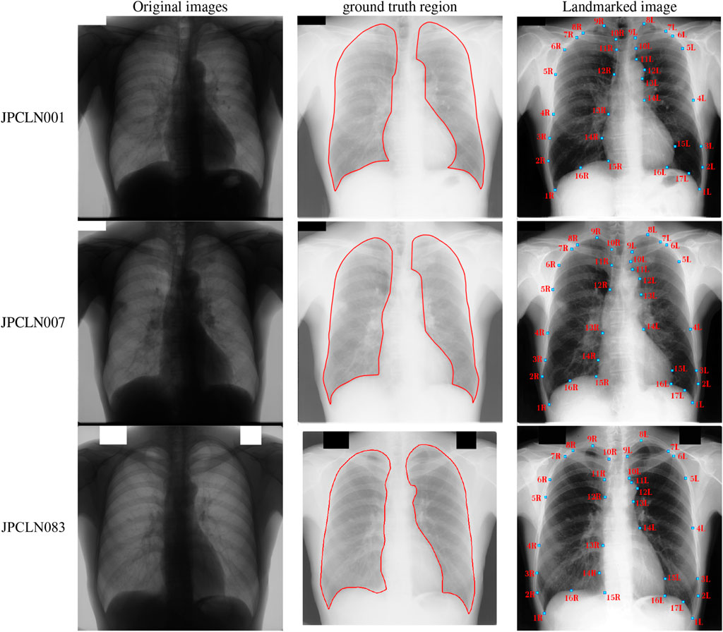
FIGURE 1. Selected images from JSRT dataset, ground truth of the left and right lung field regions, and the placement of manually annotated anatomical landmark points after negative transformation.

4.1 Evaluation Metrics

In order to compare the different interpolation techniques, two different performance measures, namely, Jaccard similarity coefficient and Dice similarity coefficient [38], are used that evaluate the quality of delineation and interpolation.

1) Jaccard similarity coefficient (JSC): the Jaccard similarity coefficient or Jaccard index (J) between the ground truth shape and the interpolated shape is defined as

$J=\frac{|S_{IS}\cap S_{GT}|}{|S_{IS}\cup S_{GT}|}(37)$

2) Dice coefficient (DC): the Dice coefficient between the ground truth shape and interpolated shape is defined as

$D=2\frac{|S_{IS}\cap S_{GT}|}{|S_{IS}|+|S_{GT}|}(38)$

where S_GT is the region enclosed by the ground truth shape and S_IS is the region enclosed by the interpolated shape. The Jaccard coefficient and Dice coefficient between the two shape instances give us an idea of how similar the two sets are. The JSC and DC take a value between $\left[\mathrm{0,1}\right]$. The zero indicates that the two shape instances do not coincide with each other, whereas one indicates that the two shape instances completely coincide with each other.

3) Execution time: estimating the execution time often becomes mandatory when evaluating the performance of an algorithm. Knowledge about the execution time of program is of utmost importance in selecting an appropriate method that models the lung field shape within a specified amount of time. The polynomials that take a longer time than the specified amount of time cannot be preferred for the lung field modeling.

5 Simulation Result

In this work, five different interpolating polynomials are studied for the left and right lung field modeling using a set of discrete labeled points called anatomical landmark points. For this purpose, three similar radiographs from the publicly available JSRT dataset are selected. We identified and selected 17 anatomical landmark points for the left lung region and 16 anatomical landmark points for the right lung region in the selected set of images, as shown in Figure 1. As the selected landmark points are not sufficient to form the lung contour, piecewise interpolating polynomials are used to create additional intermediate semilandmark points between each pair of the consecutive landmark points. Our intention is to get a shape of highest similarity index by interpolating minimum number of the secondary landmark points (i.e., intermediate semilandmarks). Hence, an analysis is made to find a shape of highest similarity index by interpolating a minimum number of intermediate semilandmark points. For this purpose, the piecewise interpolating polynomials are used for obtaining 1–15 intermediate semilandmark points between each pair of the consecutive landmark points. Performance of each interpolating polynomial is evaluated for intermediate semilandmarks—varying in number from 1 to 15—formed between each pair of the consecutive landmark points. Figure 2 shows the lung shape modeling of the image data set JPCLN001 using selected interpolating polynomials with linear, cubic convolution, cubic spline, PCHIP, and Makima interpolation methods, respectively, using one, three, and ten intermediate semilandmark point(s). A similar attempt is also made to represent two other sets of images in Figures 3, 4 with the selected interpolating polynomials using one, three, and ten secondary landmark point(s). Here, red and green contours are used to represent ground truths and lung field boundaries obtained using different interpolating polynomials, respectively. Performance of each interpolation method is evaluated, for the left and right lung field modeling, against the number of intermediate semilandmark points, in terms of Jaccard similarity coefficient and Dice coefficient. Figure 5 shows the performance of each interpolating polynomial in terms of Jaccard similarity coefficient and Figure 6 is used to represent their performance in terms of Dice coefficient. A tabular form of the different interpolating polynomials for which Jaccard’s and Dice’s coefficients remain optimal with the minimum required condition is shown in Table 1. Here, optimality refers to a situation in which JSC and DC attain the best or most favorable value beyond which no such significant change is sought. The optimality condition refers to a condition that is required (in terms of the minimum number of intermediate semilandmark points between each consecutive anatomical landmark pair) for the JSC and DC to attain the best or most favorable value. The execution time of these interpolating polynomials is evaluated for the three intermediate semilandmark points and is shown and compared in Figure 7. The simulation work is carried out using MATLAB R2018b installed under the Fedora Linux kernel version 5.6.13-300.fc32.x86_64 in HP ENVY 15-k004tx Notebook PC with the configuration of 1.7 GHz Intel Core i5-4210U processor having Intel HD Graphics 4400 and 8 GB of RAM.

FIGURE 2

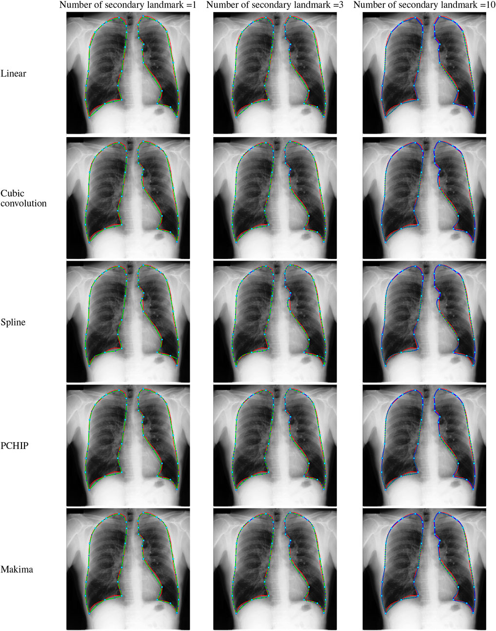
FIGURE 2. Lungs region formation: ground truth (red) and the modeled shape (green) using different interpolating polynomials with 1, 3, and 10 intermediate semilandmark point(s) of the selected image dataset JPCLN001.

FIGURE 3

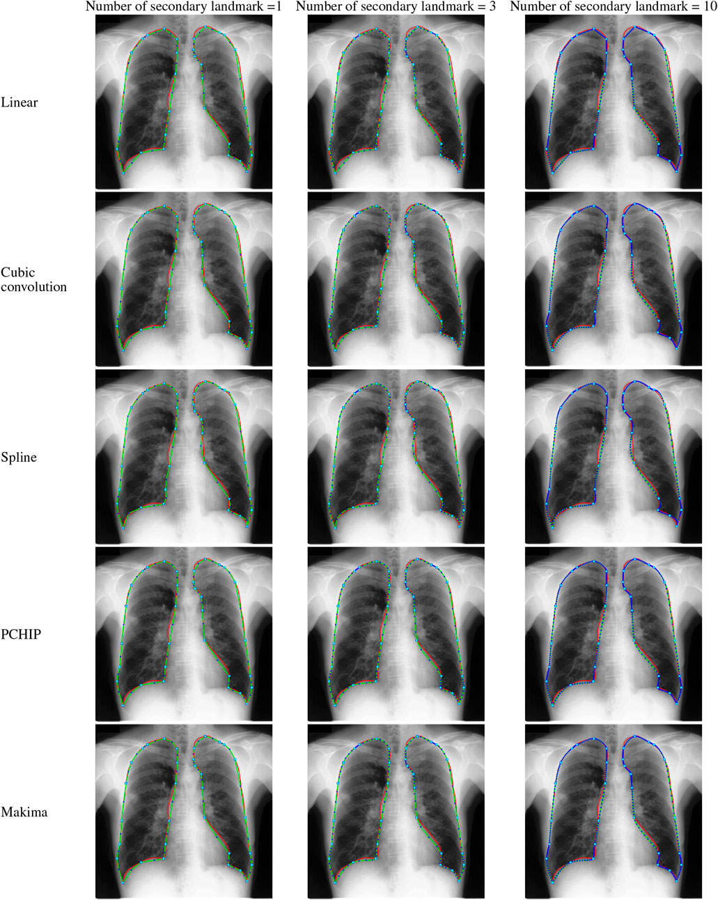
FIGURE 3. Lungs region formation: ground truth (red) and the modeled shape (green) using different interpolating polynomials with 1, 3, and 10 intermediate semilandmark point(s) of the selected image dataset JPCLN007.

FIGURE 4

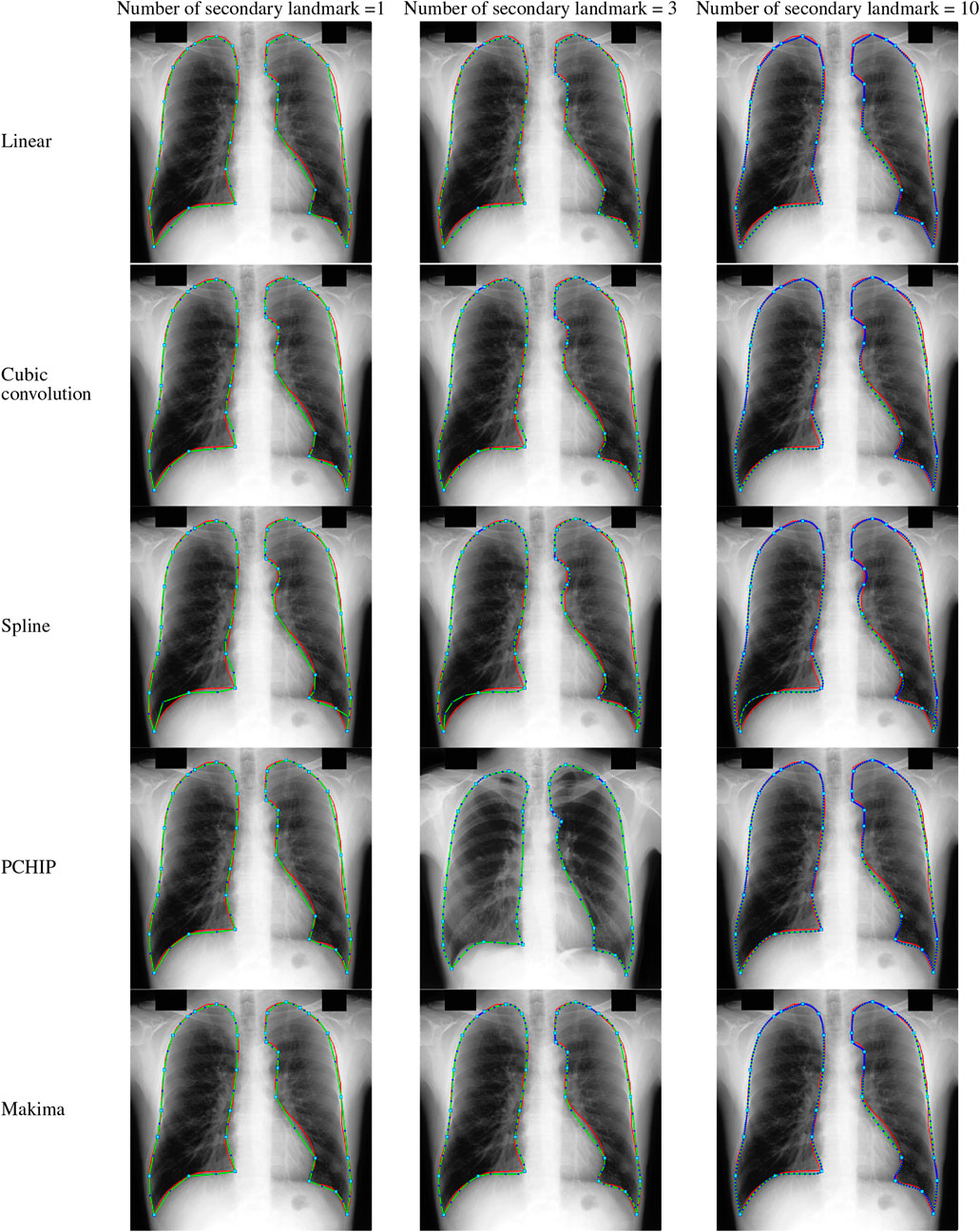
FIGURE 4. Lungs region formation: ground truth (red) and the modeled shape (green) using different interpolating polynomials with 1, 3, and 10 intermediate semilandmark point(s) of the selected image dataset JPCLN083.

FIGURE 5

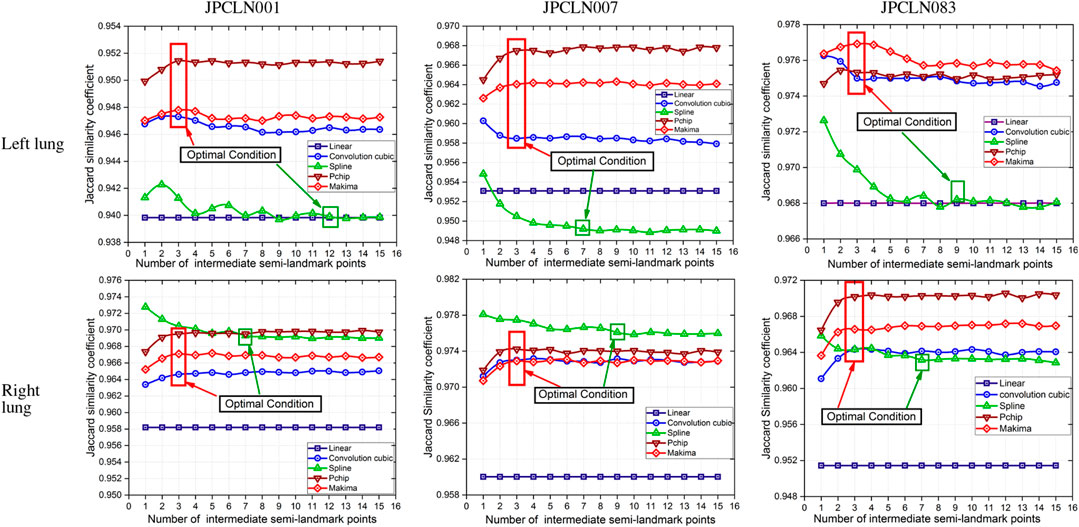
FIGURE 5. Jaccard similarity coefficients of the modeled shape with different piecewise polynomial interpolation methods of the left and right lung field regions of the image datasets JPCLN001, JPCLN007, and JPCLN083.

FIGURE 6

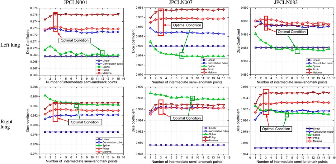
FIGURE 6. Dice similarity coefficients of the modeled shape with different piecewise polynomial interpolation methods of the left and right lung field regions of the image datasets JPCLN001, JPCLN007, and JPCLN083.

TABLE 1

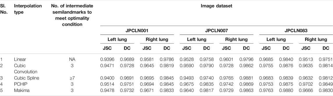
TABLE 1. Jaccard’s and Dice’s coefficients of different interpolation schemes with their optimality condition.

FIGURE 7

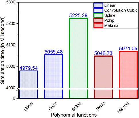
FIGURE 7. Simulation time of different interpolating polynomials.

6 Conclusion

Here, we have presented an effective method of anatomical landmark point selection and their minimization and modeling of the lung field shape using five different interpolation techniques, namely, linear, cubic convolution, cubic spline, PCHIP, and Makima. Each interpolation method is applied locally with a certain number of intermediate semilandmark point(s) between each consecutive anatomical landmark pair. We measured and compared the modeling performance of each interpolation technique with the prepared ground truth in terms of Jaccard similarity coefficient (JSC) and Dice coefficient (DC). The modeled shape using linear interpolation method with an execution time of 4.97954 s ensures a shape of minimum similarity index (with an average JSC of 95.36 and 95.65% and with an average DC of 97.62 and 97.78% for the left and right lung fields, respectively) and has no impact of increasing the number of intermediate semilandmark points. Therefore, optimality condition for the linear interpolation method cannot be defined. However, for PCHIP and Makima interpolation methods, an incremental change in JSC and DC is observed as the number of intermediate semilandmark points between each consecutive anatomical landmark pair increases from one to three intermediate semilandmark point(s). As soon as the number of intermediate semilandmark points increases beyond three, no significant change in JSC and DC is observed. Hence, with a minimum of three intermediate semilandmark points, the JSC and DC reach the optimal value in case of PCHIP and Makima interpolation methods with an execution time of 5.04873 and 5.07105 s, respectively. The case with cubic convolution is no exception to this and here also the optimal values of JSC and DC are attained with a minimum of three intermediate semilandmark points with an execution time of 5.05548 s irrespective of the incremental or decremental change between one and three intermediate semilandmark point(s). The cubic spline method, however, does not follow the same trend and a gradual decrease or damping is observed in JSC and DC when the number of intermediate semilandmark points is below seven. The cubic spline method takes at least seven intermediate semilandmark points to produce an optimum result. From the experimentation, it is concluded that the PCHIP interpolation method is the most promising candidate for shape modeling of the lung field region with an average JSC of 96.47 and 97.13% and with an average DC of 98.20 and 98.54% for the left and right lung fields, respectively, with the optimality condition of three intermediate semilandmark points. The Makima interpolation method is not far behind and it modeled the shape with an average JSC of 96.27 and 96.87% and with an average DC of 98.10 and 98.42% for the left and right lung fields, respectively, with the optimality condition of three intermediate semilandmark points. The cubic convolution interpolation method takes an average JSC of 96.05 and 96.69% and average DC of 97.98 and 98.32% for the left and right lung field modeling, respectively, with the optimality condition of three intermediate semilandmark points. In contrary to the above stated methods that have the optimality condition of three intermediate semilandmark points, the cubic spline method takes an average JSC of 95.25 and 96.97% and an average DC of 97.56 and 98.46% for the left and right lung field modeling, respectively, with the optimality condition of at least seven intermediate semilandmark points. The cubic spline method remains the weakest candidate for the lung field modeling due to longer execution time of 5.22529 s for the three intermediate semilandmark points and the high optimality condition of at least seven intermediate semilandmark points.

Data Availability Statement

The original contributions presented in the study are included in the article/Supplementary Material; further inquiries can be directed to the corresponding author.

Author Contributions

RK and SB conceived of the presented idea. RK developed the theory and performed the computations. GM verified the analytical methods. SB investigated (a specific aspect) and supervised the findings of this work. All authors discussed the results and contributed to the final manuscript.

Conflict of Interest

The authors declare that the research was conducted in the absence of any commercial or financial relationships that could be construed as a potential conflict of interest.

Publisher’s Note

All claims expressed in this article are solely those of the authors and do not necessarily represent those of their affiliated organizations, or those of the publisher, the editors, and the reviewers. Any product that may be evaluated in this article, or claim that may be made by its manufacturer, is not guaranteed or endorsed by the publisher.

Acknowledgments

The authors would like to thank Dr. Rajeev Nayan, MD, Radiology, Relief Diagnostic Centre, Dhanbad, Jharkand (India), for the manual annotation and ground truth preparation of the image dataset.

References

1. Jaeger S, Karargyris A, Candemir S, Folio L, Siegelman J, Callaghan F, et al. Automatic Tuberculosis Screening Using Chest Radiographs. IEEE Trans Med Imaging (2013) 33:233–45. doi:10.1109/TMI.2013.2284099

PubMed Abstract | CrossRef Full Text | Google Scholar

2. Shariaty F, Mousavi M. Application of CAD Systems for the Automatic Detection of Lung Nodules. Inform Med Unlocked (2019) 15:100173. doi:10.1016/j.imu.2019.100173

CrossRef Full Text | Google Scholar

3. Cao W, Wu R, Cao G, He Z. A Comprehensive Review of Computer-Aided Diagnosis of Pulmonary Nodules Based on Computed Tomography Scans. IEEE Access (2020) 8:154007–23. doi:10.1109/access.2020.3018666

CrossRef Full Text | Google Scholar

4. Mittal A, Hooda R, Sofat S. Lung Field Segmentation in Chest Radiographs: A Historical Review, Current Status, and Expectations from Deep Learning. IET Image Process (2017) 11:937–52. doi:10.1049/iet-ipr.2016.0526

CrossRef Full Text | Google Scholar

5. Cootes TF, Taylor CJ. Active Shape Models - 'Smart Snakes'. BMVC (1992) 266–75. doi:10.1007/978-1-4471-3201-1_28

CrossRef Full Text | Google Scholar

6. Cootes TF, Taylor CJ, Cooper DH, Graham J. Active Shape Models-Their Training and Application. Computer Vis Image Understanding (1995) 61:38–59. doi:10.1006/cviu.1995.1004

CrossRef Full Text | Google Scholar

7. Zheng G, Gollmer S, Schumann S, Dong X, Feilkas T, González Ballester MA. A 2D/3D Correspondence Building Method for Reconstruction of a Patient-Specific 3D Bone Surface Model Using Point Distribution Models and Calibrated X-ray Images. Med image Anal (2009) 13:883–99. doi:10.1016/j.media.2008.12.003

PubMed Abstract | CrossRef Full Text | Google Scholar

8. van Ginneken B, Stegmann MB, Loog M. Segmentation of Anatomical Structures in Chest Radiographs Using Supervised Methods: A Comparative Study on a Public Database. Med Image Anal (2006) 10:19–40. doi:10.1016/j.media.2005.02.002

PubMed Abstract | CrossRef Full Text | Google Scholar

9. Iakovidis DK, Papamichalis G. Automatic Segmentation of the Lung Fields in Portable Chest Radiographs Based on Bazier Interpolation of Salient Control Points. In: 2008 IEEE International Workshop on Imaging Systems and Techniques. IEEE (2008). p. 82–7.

Google Scholar

10. Shao Y, Gao Y, Guo Y, Shi Y, Yang X, Shen D. Hierarchical Lung Field Segmentation With Joint Shape and Appearance Sparse Learning. IEEE Trans Med Imaging (2014) 33:1761–80. doi:10.1109/TMI.2014.2305691

PubMed Abstract | CrossRef Full Text | Google Scholar

11. Wu G, Zhang X, Luo S, Hu Q. Lung Segmentation Based on Customized Active Shape Model From Digital Radiography Chest Images. J Med Imaging Hlth Inform (2015) 5:184–91. doi:10.1166/jmihi.2015.1382

CrossRef Full Text | Google Scholar

12. Li X, Luo S, Hu Q, Li J, Wang D, Chiong F. Automatic Lung Field Segmentation in X-ray Radiographs Using Statistical Shape and Appearance Models. J Med Imaging Hlth Inform (2016) 6:338–48. doi:10.1166/jmihi.2016.1714

CrossRef Full Text | Google Scholar

13. Cheimariotis G-A, Al-Mashat M, Haris K, Aletras AH, Jögi J, Bajc M, et al. Automatic Lung Segmentation in Functional SPECT Images Using Active Shape Models Trained on Reference Lung Shapes from CT. Ann Nucl Med (2018) 32:94–104. doi:10.1007/s12149-017-1223-y

PubMed Abstract | CrossRef Full Text | Google Scholar

14. Mansoor A, Cerrolaza JJ, Perez G, Biggs E, Okada K, Nino G, et al. A Generic Approach to Lung Field Segmentation From Chest Radiographs Using Deep Space and Shape Learning. IEEE Trans Biomed Eng (2019) 67:1206–20. doi:10.1109/TBME.2019.2933508

PubMed Abstract | CrossRef Full Text | Google Scholar

15. Cerrolaza JJ, Reyes M, Summers RM, González-Ballester MÁ, Linguraru MG. Automatic Multi-Resolution Shape Modeling of Multi-Organ Structures. Med image Anal (2015) 25:11–21. doi:10.1016/j.media.2015.04.003

PubMed Abstract | CrossRef Full Text | Google Scholar

16. El-Rewaidy H, Nezafat M, Jang J, Nakamori S, Fahmy AS, Nezafat R. Nonrigid Active Shape Model-Based Registration Framework for Motion Correction of Cardiac T1mapping. Magn Reson Med (2018) 80:780–91. doi:10.1002/mrm.27068

PubMed Abstract | CrossRef Full Text | Google Scholar

17. Spinczyk D, Krasoń A. Automatic Liver Segmentation in Computed Tomography Using General-Purpose Shape Modeling Methods. Biomed Eng Online (2018) 17:65–13. doi:10.1186/s12938-018-0504-6

PubMed Abstract | CrossRef Full Text | Google Scholar

18. Pingkun Yan P, Sheng Xu S, Turkbey B, Kruecker J. Discrete Deformable Model Guided by Partial Active Shape Model for TRUS Image Segmentation. IEEE Trans Biomed Eng (2010) 57:1158–66. doi:10.1109/tbme.2009.2037491

PubMed Abstract | CrossRef Full Text | Google Scholar

19. Kumar R. Analysis of Shape Alignment Using Euclidean and Manhattan Distance Metrics. In: 2017 International Conference on Recent Innovations in Signal processing and Embedded Systems. RISE IEEE (2017). p. 326–31. doi:10.1109/rise.2017.8378175

CrossRef Full Text | Google Scholar

20. Lehmann TM, Gönner C, Spitzer K. Survey: Interpolation Methods in Medical Image Processing. IEEE Trans Med Imaging (1999) 18:1049–75. doi:10.1109/42.816070

PubMed Abstract | CrossRef Full Text | Google Scholar

21. Blu T, Thévenaz P, Unser M. Linear Interpolation Revitalized. IEEE Trans Image Process (2004) 13:710–9. doi:10.1109/TIP.2004.826093

PubMed Abstract | CrossRef Full Text | Google Scholar

22. Keys RG. Cubic Convolution Interpolation for Digital Image Processing. IEEE Trans Acoust Speech, Signal Process (1981) 29. doi:10.1109/tassp.1981.1163711

CrossRef Full Text | Google Scholar

23. Zhou D, Dong W, Shen X. Image Zooming Using Directional Cubic Convolution Interpolation. IET Image Process (2012) 6:627–34. doi:10.1049/iet-ipr.2011.0534

CrossRef Full Text | Google Scholar

24. Meijering E, Unser M. A Note on Cubic Convolution Interpolation. IEEE Trans Image Process (2003) 12:477–9. doi:10.1109/TIP.2003.811493

PubMed Abstract | CrossRef Full Text | Google Scholar

25. Hsieh Hou HS, Andrews H. Cubic Splines for Image Interpolation and Digital Filtering. IEEE Trans Acoust Speech, Signal Process (1978) 26:508–17. doi:10.1109/TASSP.1978.1163154

CrossRef Full Text | Google Scholar

26. Dyer SA, Dyer JS. Cubic-Spline Interpolation. 1. IEEE Instrum Meas Mag (2001) 4:44–6. doi:10.1109/5289.911175

CrossRef Full Text | Google Scholar

27. Abdul Karim SA, Voon Pang K. Shape Preserving Interpolation Using Rational Cubic Spline. J Appl Mathematics (2016) 2016. doi:10.1155/2016/4875358

CrossRef Full Text | Google Scholar

28. Karim S. Rational Cubic Spline Interpolation for Monotonic Interpolating Curve With C2 Continuity. MATEC Web Conferences (EDP Sciences) (2017) 131:4016. doi:10.1051/matecconf/201713104016

CrossRef Full Text | Google Scholar

29. Fritsch FN, Carlson RE. Monotone Piecewise Cubic Interpolation. SIAM J Numer Anal (1980) 17:238–46. doi:10.1137/0717021

CrossRef Full Text | Google Scholar

30. McGregor G, Nave J-C. Area-preserving Geometric Hermite Interpolation. J Comput Appl Mathematics (2019) 361:236–48. doi:10.1016/j.cam.2019.03.005

CrossRef Full Text | Google Scholar

31. Rabbath CA, Corriveau D. A Comparison of Piecewise Cubic Hermite Interpolating Polynomials, Cubic Splines and Piecewise Linear Functions for the Approximation of Projectile Aerodynamics. Defence Technology (2019) 15. doi:10.1016/j.dt.2019.07.016

CrossRef Full Text | Google Scholar

32. Akima H. A New Method of Interpolation and Smooth Curve Fitting Based on Local Procedures. J Acm (1970) 17:589–602. doi:10.1145/321607.321609

CrossRef Full Text | Google Scholar

33. Ionita C, Moler C. Makima Piecewise Cubic Interpolation. Cleve’s Corner: Cleve Moler On Mathematics And Computing MATLAB & Simulink (2019). (Accessed: Mar 10, 2020)

Google Scholar

34. Moler CB. Numerical Computing with Matlab, Chapter: 3. Interpolation. Society for Industrial and Applied Mathematics (SIAM). Philadelphia. (Accessed: March 10, 2020), (2000) 93–116. doi:10.1137/1.9780898717952.ch3

CrossRef Full Text | Google Scholar

35. Shiraishi J, Katsuragawa S, Ikezoe J, Matsumoto T, Kobayashi T, Komatsu K-i., et al. Development of a Digital Image Database for Chest Radiographs with and without a Lung Nodule. Am J Roentgenology (2000) 174:71–4. doi:10.2214/ajr.174.1.1740071

CrossRef Full Text | Google Scholar

36. Coche EE, Ghaye B, de Mey J, Duyck P. Comparative Interpretation of CT and Standard Radiography of the Chest. New York, NY: Springer Science & Business Media (2011).

Google Scholar

37. Tack D, Howarth N. Missed Lung Lesions: Side-By-Side Comparison of Chest Radiography with MDCT, 15th International Annual Conference, CNCERT 2018 (2019), Beijing, China:17, 26. doi:10.1007/978-3-030-11149-6_2

CrossRef Full Text | Google Scholar

38. Yang W, Liu Y, Lin L, Yun Z, Lu Z, Feng Q, et al. Lung Field Segmentation in Chest Radiographs From Boundary Maps by a Structured Edge Detector. IEEE J Biomed Health Inform (2017) 22:842–51. doi:10.1109/JBHI.2017.2687939

PubMed Abstract | CrossRef Full Text | Google Scholar