 Pablo Serna
 Miguel Ortuño
 Andrés M. Somoza
- Departamento de Física—CIOYN, Universidad de Murcia, Murcia, Spain
We obtain eigenstates of interacting disorder Hamiltonians using unitary displacement transformations that rotate the state of the system. The method generates excited states if the strength of these transformations is chosen to optimize the energy, while decreasing the energy variance. We apply the method to analyse the localization properties of one-dimensional spinless fermions with short range interactions, reaching relatively large system sizes. We quantify the degree of localization through the size and disorder dependence of the inverse participation ratio.
1 Introduction
In strongly disordered interacting systems, particles are localized, a phenomenon known as many-body localization (MBL) [1–6]. MBL can be understood through the existence of an extensive number of exponentially localized integrals of motion (IOM) [7–10]. A practical computational approach to obtain the IOM and diagonalize interacting fermionic Hamiltonians was developed with the help of displacement transformations [11, 12], a type of unitary transformation (see Eq. 2). A similar method to diagonalize these Hamiltonians [13] had been previously introduced in a different context.
In a previous publication [14], two of us together with Louk Rademaker improved the numerical efficiency of the displacement transformations technique by focusing on a specific reference state and considering only those transformations that affect the energy of this state. In the present work, the spotlight is again on a reference state, but instead of diagonalising the Hamiltonian, we rotate the state of the system. As we will see, this further increases the efficiency of the method. One of the reasons for this increase is that storing a state is less expensive than storing a transformed Hamiltonian. We focus on the effect of the most influential displacement transformations to gain information on the localization properties of the state. The method proposed in this work is quite general, fairly easy to implement and it may be of interest in different fields, such as quantum chemistry, nuclear physics, Rydberg atoms and molecules, quantum spins, etc.
The flow equation method [15–21] is a continuous versions of our model, in which a set of differential equations is solved to implement the displacement transformations. Continuous transformations have the advantage of commuting one with each other for infinitesimal strengths, while discrete implementations take into account the term to be transformed at all orders in a single step. Besides, discrete transformations can handle better the storage of the states, which can be done in a sparse representation. This opens the possibility of reaching larger system sizes.
The remainder of the paper is set up as follows. In section 2 we present the Hamiltonian considered and briefly review the definition and main property of displacement transformations. In section 3 we deduce the equations to minimize the energy with displacement transformations for a general state. We then describe how to obtain excited states in section 4 and analyse their localization properties in 5. In section 6 we discuss possible applications and extract some conclusions.
2 Model Hamiltonian and Displacement Transformations
Although our method applies to any fermionic quantum Hermitian Hamiltonian, we concentrate on the one-dimensional tight-binding Anderson interacting Hamiltonian
where c†i (ci) is the fermionic creation (annihilation) operator of state i and ni = c†ici is the number operator. ϕi are the site energies, distributed uniformly in the interval (−W/2, W/2), t is the hopping energy, ⟨i, j⟩ refers to nearest neighbours, and Ui,j the interaction. The method works for any type of interaction, and here we will only consider a nearest neighbour interaction Ui,j = U0δi,i+1.
For an operator X containing the same number of creation and annihilation operators we can define the following unitary transformation
This is called a displacement transformation of strength λ for the operator X. And the total number of creation and annihilation operators in X is called the order of the transformation. The Hamiltonian given by Eq. 1 can be diagonalized by products of displacement transformations [11], ending up of the form
ñ is the transform of the density operator under the same transformation performed on the Hamiltonian.
It is trivial to show that displacement transformations can be summed up, given that X3 = X, in the following compact way
where 1 is the unit operator.
3 Energy Minimization
As we have mentioned, one can in principle diagonalize the Hamiltonian by the application of successive displacement transformations [11, 12], but in this process high order terms in the Hamiltonian are generated and to store them for large sizes is a real challenge. An alternative approach is to focus on a given state |Φ⟩ and perform only those transformations that affect the expectation value or the variance of the Hamiltonian with respect to this state. The expectation value of the energy after a transformation
where A ≡ X† − X and expectation values are computed with respect to state |Φ⟩. In a previous work [14], we optimized the expectation value of the energy by applying the displacement transformations to the Hamiltonian, while keeping the state fixed. In the present study we keep the Hamiltonian fixed and apply the transformations to the state. The final state will be
When the state is kept fixed, it is normal to consider a single component state (possibly in the complex basis defined by the integrals of motion), and the only transformations that affect the energy expectation value satisfy ⟨A2⟩ = − 1. In the general case, we can no longer assume this condition and Eq. 5 can be written as:
where
To obtain these quantities for a given X, we compute the auxiliary states |Φ1⟩ = A|Φ⟩ and |Φ2⟩ = A2|Φ⟩ and from them we evaluate the action of the Hamiltonian operator on them, H|Φ1⟩ and H|Φ2⟩. All quantities appearing in Eqs 8–11 are scalar products of the four states just mentioned. The task that requires most of the CPU time is the evaluation of H|Φ1⟩ and H|Φ2⟩.
The function given by Eq. 7 has period π, and there is always an extreme of the energy between − π/2 and π/2. To get excited states, we choose the extreme corresponding to the minimum value of |λ|, since this is the most effective strategy to get as many excited states as possible, as we will see. Once we have the value of λ, the calculation of the transformed state is straight forward
The energy is an extreme for all eigenvalues, but not necessarily a minimum, except for the ground state. So, to avoid stability problems for excited states, we reject transformations that increase the variance of the energy. This quantity is calculated from its definition.
The two expectation values on the right hand side of this equation are evaluated according to Eq. 7.
The previous procedure can be implemented for any one-electron basis. The two most obvious choices are the site basis and the solution of the one-electron problem. In the site basis, the Hamiltonian takes a very simple form and it is very efficient to evaluate its action on a wavefunction. On the other hand, wavefunctions always have a very large number of components. The second possibility, the solution of the one-electron problem, involves a more complicated form of the Hamiltonian and wavefunctions whose effective number of components varies drastically between the localized and the extended regime. We will call this basis the non-interacting basis and we will work with it for the reasons given later on. To avoid confusion, we refer to states in the non interacting basis with greek letters. In this basis the Hamiltonian is
4 Excited States
Our main aim is to obtain excite states with as little bias as possible and study their localization properties. To get these states is not a trivial task and, for example, starting from a canonical basis in the site occupation a large proportion of the final states coalesce in a few states. We have tested several different strategies to obtain as many excited states as possible. The best we have found is the following:
1. The initial state is a single component state on the non-interacting basis. Up to system size L = 16 we run over all possible initial states. For larger systems, we choose initial states at random.
2. Successive displacement transformations are applied to the state, choosing the minimum absolute value of the strength λ that minimizes or maximizes the energy. Transformations that increase the variance of the energy are rejected.
As the calculation of λ, for a given X, involves a CPU time similar to the transformation of the state, it is convenient to choose first the operators X that we think are likely to be more important, i.e., that correspond to larger values of |λ|. We order the operators X according to
We have only considered fourth order X operators. after all displacement transformations for fourth order operators has been performed, we consider again the same set of operators, which now produce displacement transformations with much smaller values of the strength λ. The whole procedure is repeated three times and we have checked that after this, convergence is basically achieved.
The displacement transformations that increase the energy variance and so are rejected depend on the state considered. They appear at late stages, when the rotations of the corresponding operators have already been performed at least once.
We can express a general state |Ψ⟩ as a linear combination of configurations (Slater determinants) |ΦΘ⟩ in a given basis:
Each configuration is represented by an integer, whose 0’s and 1’s in its binary form corresponds to the empty and occupied states of the configuration. A state is represented by a set of configurations and the corresponding weights aΘ.
In the rest of the paper, we consider a nearest neighbour interaction with U = 1, which sets our unit of energy, a transfer energy t = 1/2. We fix the total number of particles to half the number of sites. For this model, the ground state is always localized, while we expect to have a delocalization transition at infinite temperature for a critical disorder around Wc ≈ 4 [22–25] in our units, although it could be a larger value [26–28].
For small system sizes, we can generate all the final states starting from a complete initial standard basis and compare the results with exact diagonalization. We start from a single component state in the non-interacting basis, i.e., a Slater determinant for a given set of one-particle states. We then apply displacement transformations following the strategy described above and store the final energy of this evolved state. We arrange these energies E in ascending order and compare them with the exact energies, Eexact. The results are shown in Figure 1A for two values of the disorder W = 5 (blue) and W = 3 (orange) and system size L = 10. The larger disorder corresponds to the localized regime, while the smaller disorder to the extended regime. The black dashed line represents E = Eexact and both blue and orange curves are pretty close to it. We do not appreciate large horizontal steps, which would indicate that many initial states have collapsed into the same final state. The steps seen in Figure 1A involve a few states, while with other approaches there are large proportions of states coalescing in the same final one. In the lower part of the figure, we plot E − Eexact as a function of Eexact to appreciate better the precision of our method. Similar results to those in Figure 1A are obtained when working in the site basis. But starting from wavefunctions corresponding to Slater determinants of non interacting wavefunctions. The problem with this approach is the very large size of the wavefunction even at the very beginning of the calculation.
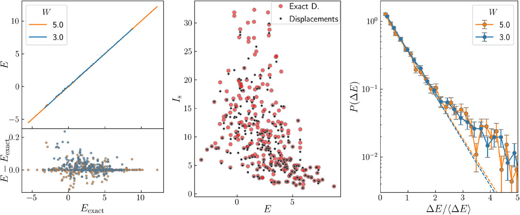
FIGURE 1. (A) Energy obtained for the different states generated with our method versus the exact energy Eexact for two values of the disorder and L = 10. Lower panel: E − Eexact versus Eexact. (B) IPR of the states in panel (A) for disorder 3 for the exact calculation and for our algorithm. (C) Energy level spacing distribution for the same parameters as in (A).
In order to check the quality of the wavefunctions obtained, rather than of the energy, we have calculated the inverse participation ratio (IPR) in the site basis, Is. The IPR is defined as
where aΘ are the components of the state, see Eq. 16. In this case, |ΦΘ⟩ correspond to a real space configuration, i.e., the set of occupied and empty sites. In Figure 1B, we compare the IPR of the states obtained in panel (a) for the exact procedure and our algorithm. The agreement for most states is good, but a few ones, mainly the least localized, present appreciable differences.
We have studied the level spacing distribution for system size L = 10. We have normalized the data to the average spacing, but not to the energy dependent average spacing, since we are only interested in its behaviour at small values. The results are presented in Figure 1C for W = 5 (blue) and W = 3 (orange) on a semilogarithmic scale. As high order displacements have not been considered, we expect the distribution to be Poisson like, independently of whether we are in the localized or in the extended regime. This is not in contradiction with Figure 1A, since very small deviations in the energies can cause an appreciable change in the level spacing. If several states were to collapse in one, we would see a peak in the level spacing distribution at small spacings [14]. No such peak can be observed in Figure 1C. To analyse this question more quantitatively, we have fitted from the second to the fifth points by a straight line, shown as a dashed line in the figure, and we see that the first point does no deviate upwards from the fitted line.
We have also analysed the behaviour of our algorithm for a larger system, L = 20. For a realization of the disorder, we consider many different initial states, i.e., Slater determinants constructed from different one-electron states, and monitor the evolution of their energy E and their energy standard deviation σ in terms of the number of displacement transformations performed. In Figure 2A we plot the evolution of the energy E for a few states as a function of the number of displacement transformations for a disorder W = 5. The shaded area around each line corresponds to E ± σ/2, and the final energy should be within this interval. The energy uncertainty in the extended regime (W = 3) is much larger than in the localized regime (W = 5), but in neither case we observe a tendency for states to merge together, at least, at a significant rate. To quantify this question, we analyse the energy level spacing as we did for L = 10. The results are shown in Figure 2C, and as before we do not appreciate a peak at very low energy spacings above the standard tendency for a Poisson distribution.
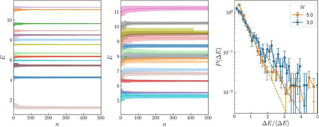
FIGURE 2. Energy as a function of the number of displacement transformations performed for several states for a disorder W = 5, panel (A), and W = 3, panel (B). The width of the shaded area is equal to the standard deviation of the energy. (C) Energy level spacing distribution for W = 5 (blue) and 3 (orange) and L = 20.
5 Localization
To study localization, we start from a single configuration state in the non-interacting basis and transform it with displacement transformations as described before. At each step, we monitor the energy variance and the IPR in the non-interacting basis, Ini. The IPR is defined as in Eq. 17, but now configurations refer to occupied and empty non-interacting states. Ini quantifies the spread of the wavefunction due to interactions. To compare our results with the IPR in the site basis, we will have to take into account the increase of the single-particle wavefunction with decreasing disorder, which is a smooth dependence.
In Figure 3A, we plot in a log-log scale the evolution of Ini for several states as displacement transformations are performed on them. In the horizontal axis we represent the energy variance of the system normalized to its initial value. Each line corresponds to the evolution of a state, and each dot to the coordinates of the state after a number of displacement transformations has been performed. Curves in orange are for W = 5 and in blue to W = 3. System size is L = 20. As displacement transformations are performed, curves evolve from right to left. The program stops when 500 transformations have been attempted (at the beginning not all transformations succeed in changing the state). In order to speed up the process, only terms larger (in absolute value) than its maximum component multiplied by 10−4 have been kept for both the Hamiltonian and the wavefunction. We note that while orange curves have basically reached an asymptotic value, most of the blue curves are still far from saturation.
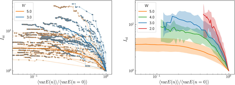
FIGURE 3. (A) Evolution of the IPR versus the normalized energy variance as displacement transformations are performed for several states in a double logarithmic scale for L = 20. Orange curves correspond to W = 5 and blue curves to W = 3. (B) Average IPR versus normalize energy variance for several values of the disorder. The width of the shaded region is equal to the IPR standard deviation.
In Figure 3B, we plot the median of Ini over 1,000 states for each of the disorders shown in the legend as a function of the normalized energy variance for size L = 20. The shaded region ranges between the 25% and the 75% of the IPR. The tendency is clear, as disorder decreases states become more extended and their IPR’s increase.
To quantify the tendency of a state to become extended, we have calculated the slope of the curves of Ini versus the normalized variance in double logarithmic scale, as those shown in Figure 3A, at different positions and have kept the maximum (absolute) value, which we denote as δ. In Figure 4A we show the histogram of this maximum slope δ for several values of W and size L = 20. Each histogram is calculated considering 600 disorder realizations and one random initial state for each realization. These histograms present a peak that increases in height and decreases in position as disorder increases. The evolution of the histograms with system size may be an adequate tool to characterize localization.
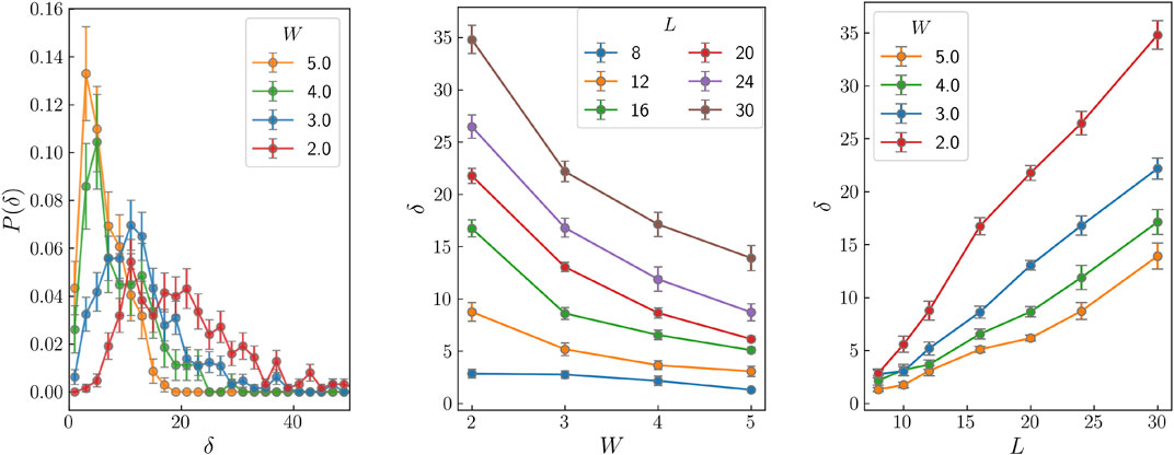
FIGURE 4. (A) Histogram of δ for several values of the disorder and L = 20. (B) Average δ versus W for several values of L. (C) Average value of δ as a function of L for the different amounts of disorder considered.
In Figure 4B we plot the average value of δ as a function of disorder for several system sizes. For disorders 2 and 3, δ drastically increases with system size, as can be seen in Figure 4C, where we represent the system size dependence of δ for the four values of the disorder considered. This is a promising tool, but we have to improve it in order to get quantitative results for the MBL transition. We are currently working on the size dependence of δ and on the relationship between the action of the displacement transformations and the dynamics.
We have also explored the effect of a cutoff in the nondiagonal terms included in the Hamiltonian on the IPR. We order these terms according to
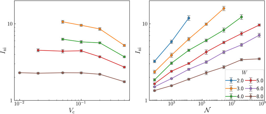
FIGURE 5. (A) Median of the IPR as a function of the cutoff in the potentials considered for several values of the disorder and system size L = 20. (B) Median of the IPR versus the size of the Hilbert space on a double logarithmic scale for several values of the disorder and L = 20.
We have calculated the IPR for several system sizes and values of the disorder using the previous cutoff Vc = 0.1. In Figure 5B we represent the results as a function of the Hilbert space, as previously done in Ref. [23], on a double logarithmic scale. Our results are consistent with those in Ref. [23] (A precise comparison is not possible, since boundary conditions are different.) We note that, within our approximations, we can reach larger system sizes.
6 Discussion and Outlook
Displacement transformations are useful to diagonalize interacting Hamiltonians. We have explored their application in two different procedures. When displacement transformations rotate the state of the system, the basis employed remain fixed along the whole process, while when one rotates the Hamiltonian, the basis is updated self-consistently at every step [14]. Rotating the Hamiltonian also has the advantage of being specially suited for renormalization techniques, but these two advantages have to be confronted with the more efficient storage of the states when these are rotated, instead of the Hamiltonian. The present implementation of the method also has the advantage of degradating its performance less with increasing system size. We believe this is due to the fact that the necessary cutoffs in the present implementation are more under control than the cutoffs in the previous one.
With the current procedure, we can reach system sizes much larger than with exact diagonalization. In this work, we have calculated up to L = 32 and we expect to reach larger sizes in the near future, at least for strong disorders, W > 4. DMRG and other approximate methods can reach large system sizes, but our approach produces large fractions of relatively unbias excited states as shown in a previous work [14]. We have checked that in the present implementation (rotating the wave-function instead of the Hamiltonian) we still reach most of the excited states.
Storing the displacement transformations utilised to get one state,
and rewrite the final state in terms of them. This is clearly an approximation, since we are only including transformations for a single state. It can be improved by considering other states.
In the site basis, the Hamiltonian takes a very simple form, but the size of the wavefunction, even the non interacting one, grows drastically with system size and renders the problem in practical for large sizes. For the calculation of the ground state, this approach is similar to that based in the ARPACK library.
Our procedure can be directly extended to any number of dimensions or to random geometries. It can also be applied to long-range interactions, and we intend to study MBL in this case. The method should be suited for molecular orbital calculations, nuclear structure determination [29], Rydberg atoms [30] and excited states in molecules [31, 32]. In the future, we would like to study the possibility of determining the localization properties from the evolution with system size of the distribution of δ.
Our method is equivalent to the Hartree-Fock approximation when displacement transformations involving only a single pair of creation and annihilation operators are performed. Including more complex transformations represents the natural extension of Hartree-Fock for the construction of non-gaussian states.
Displacement transformations constitute an excellent tool to study quantum interacting systems. In this paper, we have shown that they can be used to obtain excited states and to study their localisation properties in an efficient way.
Data Availability Statement
The original contributions presented in the study are included in the article/supplementary material, further inquiries can be directed to the corresponding author.
Author Contributions
All authors listed have made a substantial, direct, and intellectual contribution to the work and approved it for publication.
Funding
This work was supported by the Fundación Séneca grant 19907/GERM/15. MO and AS also acknowledge support from the Spanish A.E.I. grant PID2019-104272RB-C52.
Conflict of Interest
The authors declare that the research was conducted in the absence of any commercial or financial relationships that could be construed as a potential conflict of interest.
Publisher’s Note
All claims expressed in this article are solely those of the authors and do not necessarily represent those of their affiliated organizations, or those of the publisher, the editors and the reviewers. Any product that may be evaluated in this article, or claim that may be made by its manufacturer, is not guaranteed or endorsed by the publisher.
Acknowledgments
We would like to thanks Louk Rademaker for many useful discussions and his crucial contribution to the original model in which this work is based.
References
1. Basko DM, Aleiner IL, Altshuler BL. Metal-insulator Transition in a Weakly Interacting many-electron System with Localized Single-Particle States. Ann Phys (2006) 321:1126–205. doi:10.1016/j.aop.2005.11.014
2. Pal A, Huse DA. Many-body Localization Phase Transition. Phys Rev B (2010) 82:174411. doi:10.1103/PhysRevB.82.174411
3. Bardarson JH, Pollmann F, Moore JE. Unbounded Growth of Entanglement in Models of Many-Body Localization. Phys Rev Lett (2012) 109:017202. doi:10.1103/PhysRevLett.109.017202
4. De Luca A, Scardicchio A. Ergodicity Breaking in a Model Showing many-body Localization. Epl (2013) 101:37003. doi:10.1209/0295-5075/101/3700310.1209/0295-5075/101/37003
5. Abanin DA, Papić Z. Recent Progress in many-body Localization. Annalen der Physik (2017) 529:1700169. doi:10.1002/andp.201700169
6. Alet F, Laflorencie N. Many-body Localization: An Introduction and Selected Topics. Comptes Rendus Physique (2018) 19:498–525. doi:10.1016/j.crhy.2018.03.00310.1016/j.crhy.2018.03.003
7. Chandran A, Kim IH, Vidal G, Abanin DA. Constructing Local Integrals of Motion in the many-body Localized Phase. Phys Rev B (2015) 91:085425. doi:10.1103/PhysRevB.91.085425
8. Huse DA, Nandkishore R, Oganesyan V. Phenomenology of Fully many-body-localized Systems. Phys Rev B (2014) 90:174202. doi:10.1103/PhysRevB.90.174202
9. Serbyn M, Papić Z, Abanin DA. Local Conservation Laws and the Structure of the Many-Body Localized States. Phys Rev Lett (2013) 111:127201. doi:10.1103/PhysRevLett.111.12720110.1103/physrevlett.111.127201
10. Imbrie JZ, Ros V, Scardicchio A. Local Integrals of Motion in many-body Localized Systems. Annalen der Physik (2017) 529:1600278. doi:10.1002/andp.20160027810.1002/andp.201600278
11. Rademaker L, Ortuño M. Explicit Local Integrals of Motion for the Many-Body Localized State. Phys Rev Lett (2016) 116:010404. doi:10.1103/PhysRevLett.116.01040410.1103/PhysRevLett.116.010404
12. Rademaker L, Ortuño M, Somoza AM. Many‐body Localization from the Perspective of Integrals of Motion. Annalen der Physik (2017) 529:1600322. doi:10.1002/andp.201600322
13. White SR. Numerical Canonical Transformation Approach to Quantum many-body Problems. J Chem Phys (2002) 117:7472–82. doi:10.1063/1.150837010.1063/1.1508370
14. Ortuño M, Somoza AM, Rademaker L. Construction of many-body Eigenstates with Displacement Transformations in Disordered Systems. Phys Rev B (2019) 100:085115. doi:10.1103/PhysRevB.100.085115
15. Wegner FJ. Flow Equations for Hamiltonians. Phys Rep (2001) 348:77–89. doi:10.1016/S0370-1573(00)00136-8
16. Monthus C. Flow towards Diagonalization for many-body-localization Models: Adaptation of the Toda Matrix Differential Flow to Random Quantum Spin Chains. J Phys A: Math Theor (2016) 49:305002. doi:10.1088/1751-8113/49/30/30500210.1088/1751-8113/49/30/305002
17. Pekker D, Clark BK, Oganesyan V, Refael G. Fixed Points of Wegner-wilson Flows and many-body Localization. Phys Rev Lett (2017) 119:075701. doi:10.1103/PhysRevLett.119.07570110.1103/PhysRevLett.119.075701
18. Savitz S, Refael G. Stable Unitary Integrators for the Numerical Implementation of Continuous Unitary Transformations. Phys Rev B (2017) 96:115129. doi:10.1103/PhysRevB.96.11512910.1103/physrevb.96.115129
19. Monthus C. Strong Disorder Real-Space Renormalization for the many-body-localized Phase of Random Majorana Models. J Phys A: Math Theor (2018) 51:115304. doi:10.1088/1751-8121/aaad14
20. Iglói F, Monthus C. Strong Disorder RG Approach - a Short Review of Recent Developments. Eur Phys J B (2018) 91:290. doi:10.1140/epjb/e2018-90434-810.1140/epjb/e2018-90434-8
21. Thomson SJ, Schiró M. Time Evolution of many-body Localized Systems with the Flow Equation Approach. Phys Rev B (2018) 97:060201. doi:10.1103/PhysRevB.97.06020110.1103/physrevb.97.060201
22. Devakul T, Singh RRP. Early Breakdown of Area-Law Entanglement at the many-body Delocalization Transition. Phys Rev Lett (2015) 115:187201. doi:10.1103/physrevlett.115.187201
23. Macé N, Alet F, Laflorencie N. Multifractal Scalings across the many-body Localization Transition. Phys Rev Lett (2019) 123:180601. doi:10.1103/physrevlett.123.180601
24. Laflorencie N, Lemarié G, Macé N. Chain Breaking and Kosterlitz-Thouless Scaling at the many-body Localization Transition in the Random-Field Heisenberg Spin Chain. Phys Rev Res (2020) 2:042033. doi:10.1103/physrevresearch.2.042033
25. Chanda T, Sierant P, Zakrzewski J. Time Dynamics with Matrix Product States: Many-body Localization Transition of Large Systems Revisited. Phys Rev B (2020) 101:035148. doi:10.1103/physrevb.101.035148
26. Doggen EVH, Schindler F, Tikhonov KS, Mirlin AD, Neupert T, Polyakov DG, et al. Many-body Localization and Delocalization in Large Quantum Chains. Phys Rev B (2018) 98:174202. doi:10.1103/physrevb.98.174202
27. Gray J, Bose S, Bayat A. Many-body Localization Transition: Schmidt gap, Entanglement Length, and Scaling. Phys Rev B (2018) 97:201105. doi:10.1103/physrevb.97.201105
28. Sierant P, Lewenstein M, Zakrzewski J. Polynomially Filtered Exact Diagonalization Approach to many-body Localization. Phys Rev Lett (2020) 125:156601. doi:10.1103/physrevlett.125.156601
29. Szalay PG, Müller T, Gidofalvi G, Lischka H, Shepard R. Multiconfiguration Self-Consistent Field and Multireference Configuration Interaction Methods and Applications. Chem Rev (2012) 112:108–81. doi:10.1021/cr200137a
30. Gaëtan A, Miroshnychenko Y, Wilk T, Chotia A, Viteau M, Comparat D, et al. Observation of Collective Excitation of Two Individual Atoms in the Rydberg Blockade Regime. Nat Phys (2009) 5:115–8. doi:10.1038/nphys1183
31. Dreuw A, Head-Gordon M. Single-reference Ab Initio Methods for the Calculation of Excited States of Large Molecules. Chem Rev (2005) 105:4009–37. doi:10.1021/cr0505627
Keywords: localization, interaction, disorder, fermions, displacement transformations
Citation: Serna P, Ortuño M and Somoza AM (2021) Displacement Transformations as a Tool to Study Many-Body Localization. Front. Phys. 9:767001. doi: 10.3389/fphy.2021.767001
Received: 30 August 2021; Accepted: 20 October 2021;
Published: 18 November 2021.
Edited by:
Zvi Ovadyahu, Hebrew University of Jerusalem, IsraelReviewed by:
Rafael A. Molina, Consejo Superior de Investigaciones Científicas (CSIC), SpainArko Roy, University of Trento, Italy
Copyright © 2021 Serna, Ortuño and Somoza. This is an open-access article distributed under the terms of the Creative Commons Attribution License (CC BY). The use, distribution or reproduction in other forums is permitted, provided the original author(s) and the copyright owner(s) are credited and that the original publication in this journal is cited, in accordance with accepted academic practice. No use, distribution or reproduction is permitted which does not comply with these terms.
*Correspondence: Miguel Ortuño, bW9vQHVtLmVz