
95% of researchers rate our articles as excellent or good
Learn more about the work of our research integrity team to safeguard the quality of each article we publish.
Find out more
ORIGINAL RESEARCH article
Front. Phys. , 02 December 2021
Sec. Space Physics
Volume 9 - 2021 | https://doi.org/10.3389/fphy.2021.738988
This article is part of the Research Topic Micro- to Macro-Scale Dynamics of Earth’s Flank Magnetopause View all 17 articles
 E. A. Kronberg1*
 J. Gorman1,2,3
 K. Nykyri4
 A. G. Smirnov5,6,1
 J. W. Gjerloev7,8
 E. E. Grigorenko9,10L. V. Kozak11,12
 X. Ma4K. J. Trattner13M. Friel8
The Kelvin-Helmholtz instability (KHI) and its effects relating to the transfer of energy and mass from the solar wind into the magnetosphere remain an important focus of magnetospheric physics. One such effect is the generation of Pc4-Pc5 ultra low frequency (ULF) waves (periods of 45–600 s). On July 3, 2007 at ∼ 0500 magnetic local time the Cluster space mission encountered Pc4 frequency Kelvin-Helmholtz waves (KHWs) at the high latitude magnetopause with signatures of persistent vortices. Such signatures included bipolar fluctuations of the magnetic field normal component associated with a total pressure increase and rapid change in density at vortex edges; oscillations of magnetosheath and magnetospheric plasma populations; existence of fast-moving, low-density, mixed plasma; quasi-periodic oscillations of the boundary normal and an anti-phase relation between the normal and parallel components of the boundary velocity. The event occurred during a period of southward polarity of the interplanetary magnetic field according to the OMNI data and THEMIS observations at the subsolar point. Several of the KHI vortices were associated with reconnection indicated by the Walén relation, the presence of deHoffman-Teller frames, field-aligned ion beams observed together with bipolar fluctuations in the normal magnetic field component, and crescent ion distributions. Global magnetohydrodynamic simulation of the event also resulted in KHWs at the magnetopause. The observed KHWs associated with reconnection coincided with recorded ULF waves at the ground whose properties suggest that they were driven by those waves. Such properties were the location of Cluster’s magnetic foot point, the Pc4 frequency, and the solar wind conditions.
The Kelvin-Helmholtz instability (KHI) at the magnetopause has been noted for its role in the transport of mass and energy from the solar wind into the magnetosphere and down to the ground (e.g., [1–5]). The KHI has been found to occur fairly frequently under both southward and northward interplanetary magnetic field (IMF) configurations with no apparent low-speed cutoff [6,7]. When the IMF horizontal component is mostly in the Parker-Spiral orientation, the KHI has been shown to favor the dawn flank magnetopause [8].
One proposed manner in which energy transfer is achieved by the KHI is through the generation of ultra low frequency (ULF) waves. Hasegawa and Chen [9] and Southwood [1] showed theoretically that magnetic field line resonance oscillations can be caused by Kelvin-Helmholtz waves (KHWs) at the magnetopause. The observed dawnward asymmetry of Pc4-Pc5 range (frequencies of 2–22 mHz, periods of 47–600 s) ULF waves in the vicinity of the magnetopause [10] and enhanced heating of the cold-component ions at the dawn sector [11,12] are possibly related to the presence of KHI since the horizontal component of the IMF is most often in the Parker-Spiral orientation [13]. ULF waves have been shown to drive auroral arcs through magnetic field line resonance [14] and to efficiently accelerate energetic electrons in the outer radiation belt [15,16].
However, debate remains regarding whether or not the KHI is an actual, dominant driver for Pc4-Pc5 waves in the magnetosphere and at the ground [17]. Since other processes can externally drive ULF waves in the magnetosphere, it has been argued that it is likely these mechanisms that are the true drivers, occurring in conjunction with the KHI at the magnetopause. Such processes relate to high solar wind speeds and include dynamic pressure variations and foreshock fluctuation anisotropy instabilities [17]. Additionally, under southward IMF conditions other possible external drivers, such as flux transfer events, occur and interact with the KHI [18].
ULF pulsations at the magnetopause (believed to be KHWs but without explicit evidence) which were observed to propagate into the magnetosphere and down into the ionosphere in the dusk sector under fast solar wind speeds were investigated by Rae et al. [19]. Similarly, Agapitov et al. [20] presented THEMIS magnetic field observations at the dawn flank of magnetopause oscillations that coincided with ULF pulsations recorded deeper in the magnetosphere. The magnetopause surface waves were hypothesized to be KHWs based upon the critical velocity for KHI onset and wave growth [21]. Dougal et al. [22] modeled several instances of the KHI observed at the magnetospheric flanks under northward IMF to gain better insight into the resulting ionospheric signatures. Pc5 magnetic field oscillations within the ionospheric foot point ranges of some of these events were observed. Wang et al. [23] investigated magnetospheric Pc5 pulsations under steady solar wind conditions and made the case that ULF waves can not only be driven by field line resonance or waveguide modes [9], but also through the generation of inner and outer Kelvin-Helmholtz modes.
Presented herein is a Cluster-observed incidence of ULF waves in the Pc4 range observed at the magnetopause driven by the KHI associated with reconnection. The observed magnetospheric conditions were also modeled to further test if the magnetic field configuration was KHI-unstable. This event adds to the few previously published KHW-ULF linked events (e.g., [19,20,22]), but provides an even more comprehensive analysis of the magnetopause surface waves, investigating the magnetic field data in conjunction with plasma particle observations for KHI signatures at high latitudes.
Furthermore, as the present event occurs for the southward IMF orientation, according to the OMNI data and THEMIS observations at the subsolar point, both magnetic reconnection and KHI can start as a primary mode [23]. For southward IMF conditions, fast magnetic reconnection is driven and can be strongly modified by the nonlinear KH waves: MHD and Hall-MHD simulations have indicated that reconnection rates are comparable to Petschek reconnection even without the inclusion of Hall physics [24]. On the other hand, magnetic reconnection can seed the KH mode for KH unstable conditions [25]. We present evidence of north-south ULF magnetic field and plasma pressure fluctuations in the magnetosheath at the subsolar point observed by THEMIS satellites which may have modulated the KHW, and due to the additional plasma pressure compressions, may have driven the reconnection more strongly in KHI vortices. KHI vortices in our event are associated with reconnection signatures, making the case more comprehensive.
The event improves our understanding of under which conditions thin-current sheets, where reconnection can operate, are created. Identification of the processes that trigger ULF waves at the magnetospheric boundaries is important for the study of ion acceleration. Kronberg et al. [26] has demonstrated enhanced contamination of the XMM-Newton X-Ray telescope by soft protons at the flank high-latitude regions.
Finally, the satellite observed KHWs were compared with concurrent ULF pulsations measured at ground, indicating the connection between magnetic disturbances seen in space and those seen on Earth.
On July 3, 2007 from 1,645 to 1720 UT, the Cluster spacecraft approached the high-latitude dawn side magnetopause at the border between the magnetosheath and closed magnetospheric field lines (the coordinates in Geocentric Solar Ecliptic (GSE) system were X ≈ −10 RE, Y ≈ −15 RE, Z ≈ −9.4 RE). Observed plasma signatures of this event are shown in Figure 1. These measurements, which were obtained through the Cluster Science Archive [27], came from the Cluster Ion Spectrometry (CIS) experiment’s [28] COmposition and DIstribution Function (CODIF) sensor and the Hot Ion Analyser (HIA). The magnetic field components were measured by Cluster’s onboard fluxgate magnetometer (FGM) [29]. Further documentation regarding the Cluster mission can be found through Escoubet et al. [30].
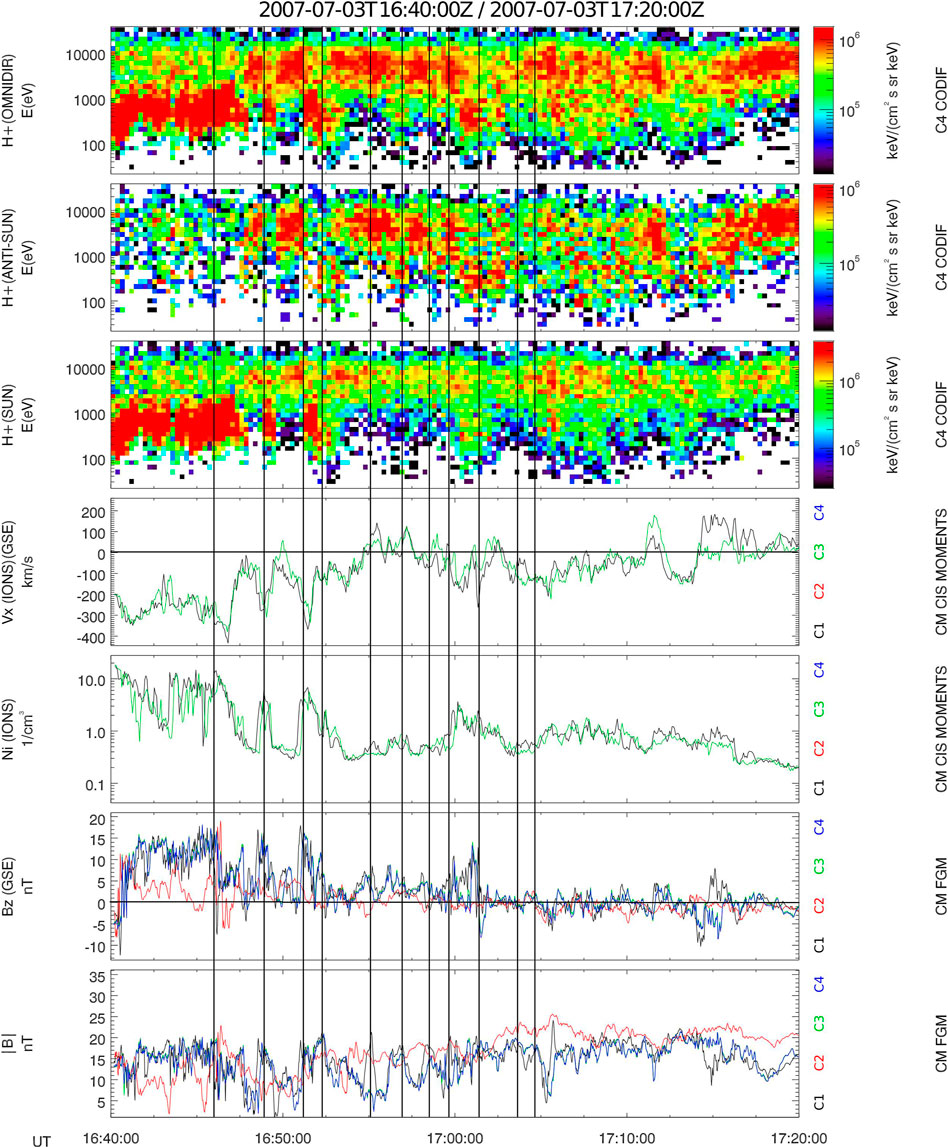
FIGURE 1. Cluster CIS observations from July 3, 2007, 1640–1,720 UT. From top to bottom: CODIF energy-time spectrograms of proton energy flux: omnidirectional, measured by the anti-sunward sensors and by the sunward sensors, in keV cm−2 s−1 sr−1 keV−1, from SC 4; ion density, cm−3, from SC 1 & 3; X-component ion velocity, km s−1 (GSE), from SC 1 & 3; Z-component and the magnitude of the magnetic field, nT (GSE), from SC 1–4. The black vertical solid lines show the times of strong maxima in the total pressure profile defined in Figure 3.
The ion density and velocity profiles measured by the CIS/HIA instrument, in conjunction with the proton energy spectrograms measured by the CIS/CODIF instrument, showed the oscillation of plasma populations (see Figure 1). Velocity fluctuations from the strongly anti-sunward to the weakly anti-sunward or sunward direction were experienced by both Cluster spacecraft (SC) 1 and 3 starting after 1645 UT (HIA data were unavailable for SC 2 and 4 during the event). The proton energy spectrograms for SC 4 displayed similar alternations between high-energy (∼ 5–10 keV) plasma typical for the magnetospheric environment and lower energy (∼ 0.3 eV–1 keV) plasma typical for the magnetosheath. Those alternations corresponded with fluctuations in the SC 1 and 3 ion densities, n, from tenuous (<1 cm−3) to dense (3–10 cm−3), respectively. These fluctuations indicate that the spacecraft were observing alternating regimes between the magnetosheath and closed magnetospheric magnetic field lines1 as expected within KHWs. The vertical, BZ, magnetic field component is strongly northward in the magnetosheath region at SC 1, 3 and 4 from 1640 to ∼1700 UT, see Figure 1. Also at these SC, the total magnetic field oscillates at the boundary between the two regimes, see discussion in Section 2.2. SC 2, which has the innermost location within the magnetosphere compared to the other SC, mainly shows higher values for the total magnetic field.
The OMNI-calculated solar wind parameters during this event can be found in Figure 2. There was a solar wind speed of ∼375 km s−1, nearly constant IMF of ∼10.5 nT and the BZ component of the IMF was southward. The wavelet analysis for wave power of the corresponding 3 s WIND data does not show any prominent spikes in the Pc4-Pc5 range (not shown). The horizontal component of the IMF was in Parker spiral orientation (BX ≈ 5 nT, BY ≈ -6 nT). There were pressure fluctuations up until about 1635 UT which then ceased and remained rather stable throughout the event time frame. The Dst index (not shown) revealed that there wasn’t a geomagnetic storm during the time of the event; however, the AE index indicated that a geomagnetic substorm had occurred.
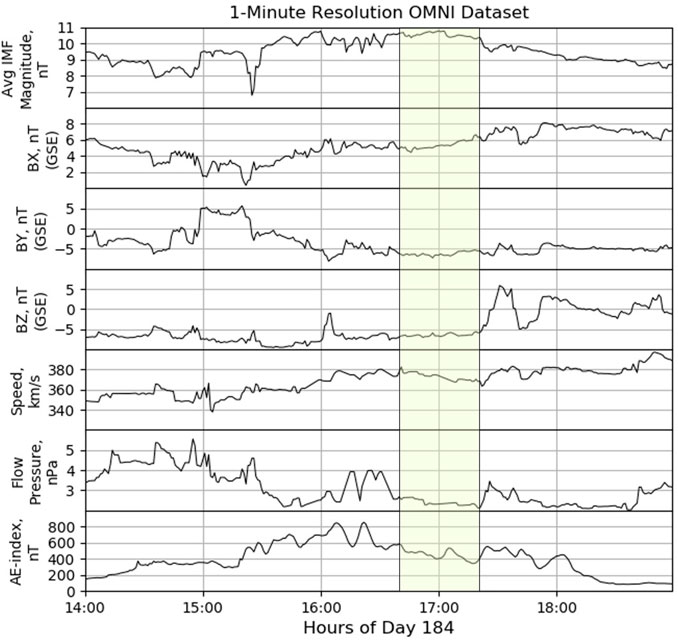
FIGURE 2. OMNI derived solar wind parameters for July 3, 2007 from 1400 to 1900 UT. The highlighted portion represents the time frame of the observed KHI from 1640 to 1720. From top to bottom: average IMF magnitude, nT; BX, nT; BY, nT; BZ, nT; speed, km s−1; flow pressure, nPa; and AE index, nT.
The profiles of velocity; magnetic field, ion density and total pressure, including its magnetic and plasma components, using Cluster SC 1 data for the time interval from 1640 to 1705 UT are shown in Figure 3. The total pressure was calculated as the sum of the magnetic (pmag) and plasma (p), calculated using observations from the CIS/HIA instrument) pressures.
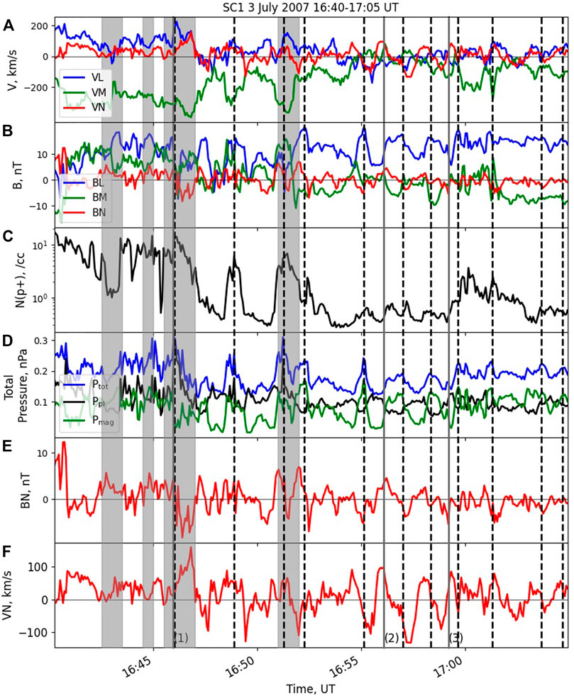
FIGURE 3. SC 1 measured and derived parameter profiles for the KHI event on July 3, 2007 are shown for the time frame of 1640–1705 UT. From top to bottom within each graph: (A) transformed velocity components L (blue), M (green) and N (red), km s−1; (B) transformed magnetic components L (blue), M (green) and N (red), nT; (C) ion density (black), cm−3; (D) total/plasma/magnetic pressure (blue/black/green), nPa; (E) transformed magnetic normal component (red), nT; (F) transformed velocity normal component (red), km s−1. The black vertical dashed lines indicate the times of strong maxima in the total pressure profile. The vertical shadowed bars show the locations of rotational discontinuities. The grey vertical solid lines denoted as (1), (2) and (3) indicate time intervals for which field-aligned beams were observed (see Figure 8).
The magnetic field and velocity data for this time interval were transformed to the (L, M, N) components which describe local boundary normal coordinate system. For this we used the Siscoe method [31]. The coordinate vectors L and M are mutually orthogonal and tangential to the boundary. N is the coordinate vector in the boundary normal direction. It is orthogonal to L and M, forming a right-handed coordinate system. The averaged values of (L, M, N) are as follows. L = [−0.62, −0.69, 0.37] and is directed mostly dawnward and tailward. M = [−0.67, 0.22, −0.71] and is directed mostly anti-sunward and southward. N = [−0.41, 0.69, 0.60] and is directed mostly duskward and northward. The eigenvalues of the system are [λ1, λ2, λ3] = [149, 46, 8]. The ratio λ2/λ3 = 5.6, indicates that the normal direction is well-defined [32]. Also, L and M are reasonably defined because λ1/λ2 = 3.2. A well-defined Siscoe normal direction was also found for SC 4 during the event (not shown).
The three dimensionality of the boundary normal relative to the GSE coordinate system, produced by complex processes at the boundary, can lead to twisting of the magnetic field in the magnetosheath in the northward direction. This can also result in a discrepancy between the southward direction as seen in the OMNI data and that observed by THEMIS-C and D at the subsolar point (not shown), see discussion in Section 5.2.
The vortex formations are indicated when the M and N coordinates are mainly in anti-phase for both the velocity and magnetic field, according to Yan et al. [33], see Figure 3. However, observations of BM and BN in anti-phase can also be associated with reconnection. As an indicator of KHI vortices, it is expected to observe anti-phase VM and VN oscillations.
In the vortex rest frame, centrifugal force moves plasma outwards from the central part of the rolled-up KHI vortices. This leads to the formation of a local minimum in total pressure at the center and a maximum at the hyperbolic point between vortices [17,34]. The hyperbolic point is also associated with the local absolute maxima of the normal magnetic field component and jumps in the density [17]. Bipolar fluctuations in the normal component of the magnetic field and flow reversals in the normal component of the velocity occurred throughout the entirety of the event, from 1645 to 1705 UT (see Figure 3). The ion density, total pressure, and other magnetic and velocity component profiles were also highly oscillatory. The vertical dashed lines mark the local total pressure maxima that are mostly aligned with the local absolute maxima of BN and with jumps in the density. This indicates the formation of the rolled-up KHI vortices (see also Discussion 5.1, (1) below).
We calculated the individual (L, M, N) coordinates for subsequent 1 min windows centered on each point in the time series, between 1640 and 1705 UT. The first panel in Figure 4 shows the values of the λ2/λ3 ratios, which are mostly well-defined throughout the event. The variation of the X, Y, and Z components of the boundary normals are also shown in Figure 4. One can see from the plot that the boundary normal is very dynamic. The angle between the averaged and individual boundary normals changes quasi-periodically in opposite directions indicating the oscillation of the boundary direction, as is typical for rolled-up KHWs.
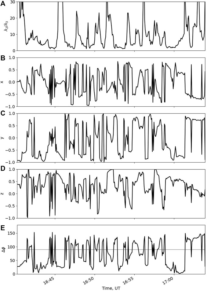
FIGURE 4. SC 1 derived parameter profiles for the KHI event on July 3, 2007 are shown for the time frame of 1640–1705 UT. From top to bottom within each graph: (A) the ratio λ2/λ3; (B–D) X, Y, and Z components of boundary normals, respectively; (E) angle between average normal and individual normal. The average normal is calculated for the whole time interval using the Siscoe method. The individual normals were defined subsequently for each 1 min period of observations. The horizontal line is at 90°.
We transformed the velocity into the deHoffmann-Teller (HT) frame, which is co-moving with the discontinuity [35]. The HT velocity,
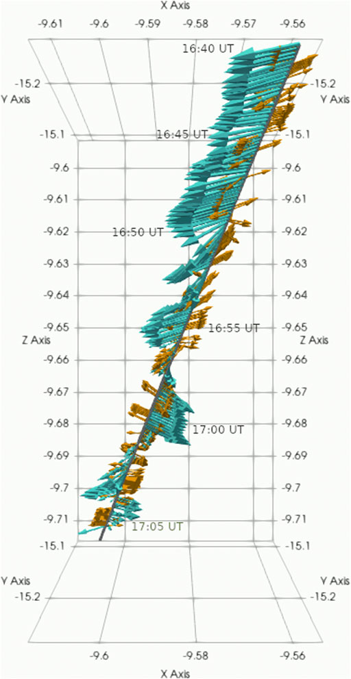
FIGURE 5. SC 1 derived observations of the HT velocity vectors (cyan) and of the boundary normals (yellow) for the KHI event on July 3, 2007 are shown for the time frame of 1640–1705 UT.
The existence of fast-moving, low-density plasma is typical for the KHI associated with mixing of two plasma environments [36,37]. We demonstrate this existence by plotting VM versus ion density in Figure 6. The color of each point indicates the ion specific entropy, S, calculated as
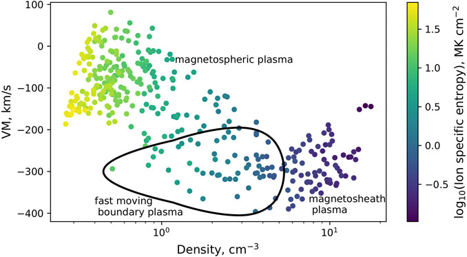
FIGURE 6. SC 1 derived observations of the VM velocity component versus ion density with colors indicating the ion specific entropy for the time frame of 1640–1705 UT.
The black line in the figure shows the fast-moving plasma population, with speeds in the range of −400 to −200 km s−1, low ion density of
The spectral wavelet analysis of the magnetic field normal fluctuations as observed by Cluster is shown in Figure 7. The periods of KHWs were defined manually using pressure maxima criteria and are marked in Figure 3 as the time between dashed lines. These periods were 173, 143, 64, 167, 113, 81, 79, 98, 142 and 62 s at ∼ 16:46:00, 16:48:53, 16:51:16, 16:52:20, 16:55:07, 16:57:00, 16:58:21, 16:59:40, 17:01:18, 17:03:40 and 17:04:42 UT, respectively. We see that the KHW-associated periods mainly coincide with power spectra increases of the magnetic field (excluding the period at 98 s, which is approximate minimum of the Fourier power spectra, and the period at 113 s, which is at the boundary between the local maximum and minimum). Within the range of marked periods we observe two power peaks in the global wavelet spectrum for the magnetic fluctuations: at periods of about 133 s and 70 s, see panel (c). These are fluctuations within the Pc4 range [39]. It seems that we observe a primary wave mode with a period ∼ 133 s and its submode at ∼ 70 s.
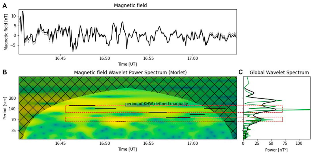
FIGURE 7. Wavelet transform analysis of Siscoe-derived magnetic field normal component, nT, from Cluster SC 1 between 16:40 and 17:05 UT: (A) original series (black) and inverse (gray) wavelet transform; (B) the normalized wavelet power spectrum and cone of influence hatched and (C) the global wavelet for periods outside of the cone of influence (COI) (black) and Fourier power spectra (green). Note that the period scale is logarithmic. The horizontal lines in panel (B) indicate periods of KHW defined manually as the time between dashed lines for corresponding time intervals in Figure 3. The dashed red rectangles correspond to two period bands from 62 to 82 s and from 113 to 173 s.
We also tested if reconnection was observed during this event. The Walén relation calculated in the HT frame shows the relation between the plasma velocity in the HT frame and the Alfvén velocity,
Field-aligned ion beams were observed at three instances during these marked intervals: 16:45:58.748 (Vpar = 2,300 kms−1, Vperp = 900 kms−1), 16:56:06.596 (Vpar = 1,400 kms−1, Vperp = − 700 kms−1) and 16:59:12.674 UT (Vpar = 1,700 kms−1, Vperp = − 500 kms−1), see Figure 8. The field-aligned beams may be an indication of ions moving along a separatrix and further imply that reconnection may have occurred. In the distribution function 1) at 1645 UT one can also simultaneously observe a perpendicular beam. This can happen if Cluster was crossing different magnetic field lines during the same data accumulation interval. The perpendicular beam can indicate that there are demagnetized ions in the reconnection exhaust region. Additionally during this interval the crescent distribution is seen, see Figure 8. This is a sign that the ions are demagnetized and the satellite was crossing the diffusion region [42]. There are multiple observations of the crescent distributions from 1640 to 1650 UT (not shown).
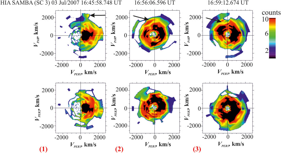
FIGURE 8. Ion velocity distribution functions as measured by the HIA instrument onboard SC 3 at 16:45:58.748 UT (left), 16:56:06.596 UT (middle) and 16:59:12.674 UT (right) during 12 s time-averaged ion velocity distribution functions. VPAR is directed along B, VPER1 is directed along − V × B and VPER2 direction completes the orthogonal system. The black arrows indicate the field-aligned beams. The time of observation for distributions (1), (2), and (3) correspond to that similarly noted in Figure 3.
During the same time period as the observed magnetopause fluctuations, large magnetic field disturbances were recorded at ground-based geomagnetic stations. These disturbances are shown in SuperMAG’s Polar Plot (Gjerloev [43]; see Figure 9). Also shown in Figure 9 is the estimated magnetic field line foot point from Cluster SC 1.
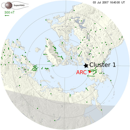
FIGURE 9. The SuperMAG Polar Plot is shown for July 3, 2007 at 1640 UT. The field line foot point corresponding to Cluster SC 1 is shown by a black star. The green vectors represent the direction and magnitude of ground-based magnetic field disturbances. The approximate location of the Arctic Station (ARC) magnetometer is denoted by the red dot.
The magnetic foot point of the Cluster mission was mapped to the ionosphere by projecting the satellite location along the magnetic field lines to the altitude of 100 km, where the lower boundary of the ionosphere was assumed. Since the spacecraft was located at the magnetosheath boundary just outside the bounds of the magnetic field model, some adjustments were necessary in order to derive the magnetic foot point’s location. In this case, the ZGSE-coordinate of the spacecraft was assumed to be equal to −8.5 RE instead of −9.6 RE, as it was the closest point where mapping was possible. The location of the magnetic foot point was derived using the Tsyganenko-1989 model of the external magnetic field [44] with internal field given by IGRF (for Kp = 2.7), as implemented in the IRBEM library [45,46]. It is worth mentioning that magnetic foot point tracing is highly model dependent (as shown in Dunlop et al. [47]) and thus gives only an approximate indication of the spacecraft position with relation to the ionosphere.
The highest amplitude of ground-measured magnetic field disturbances in the SuperMAG Polar Plots were observed to be concentrated within the North Slope region of Alaska. While magnetic fluctuations were recorded at other geomagnetic stations around the polar cap, they were lower in amplitude. The magnetic field line foot point for Cluster SC 1 mapped to the northwest coast of Canada, in the vicinity of the highest magnitude magnetic field fluctuations. Figure 10 shows the calculated magnetopause shear angle determined according to the event’s specific solar wind parameters and geomagnetic field (calculated from the T96 model [48]). The white line depicts the maximum magnetic shear angle where magnetic reconnection had the highest probability of occurring [49,50], particularly at the dawn side of the northern hemisphere. Therefore, the magnetic field fluctuations were possibly at least partially triggered by flux transfer events (FTEs) in the northern hemisphere where they are likely to occur according to Figure 10. We note that location of reconnection in Figure 10 is irrelevant to local reconnection occurring during the KHI observed by Cluster.
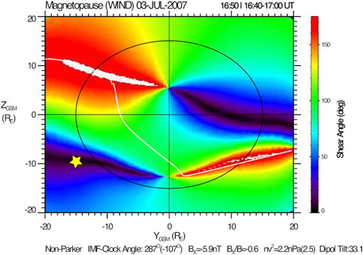
FIGURE 10. The magnetopause shear angle for IMF values BZ
Our event showed magnetic field fluctuations at the magnetopause in the Pc4 frequency range. Therefore, to establish a link between the disturbances measured by Cluster in space and those recorded at ground-based magnetic field observatories, we needed to analyze those field measurements at a resolution of 1–10°s. The closest stations to the mapped Cluster location were Arctic Village (ARC) and Kaktovik, Alaska (KAV). To show that the ARC and KAV stations were located on the closed magnetic field lines and their observations are not directly affected by the solar wind, we launched the tracing described above, using a grid with 1° steps in latitude and longitude, see the Supplementary Material S2. If the corresponding magnetic field line was closed, IRBEM returned a position of its foot point, and if the field line was open, the output was “Not a Number”. Using this information, the map of open and closed magnetic field lines was created. It can be seen from Supplementary Material S2 that the KAV and ARC stations were on closed field lines.
The wavelet analysis for the magnetic field recorded at the magnetometer in ARC (selected for its better clarity) is shown in Figure 11. The analysis shows a wave power peak in the global wavelet spectrum for the N-component at 140°s. This value approximately coincides with the main mode of the KHW. According to, for example, Hughes and Southwood [51]; Sciffer and Waters [52]; Paschmann et al. [53], not all ULF waves propagate from the magnetosphere down to the ground and the wave modes could be affected by complex wave mode conversions, modulation or damping. For instance, low ionospheric conductance during the summer could have prevented propagation of waves with periods of 70°s observed by Cluster but not observed at the ground.
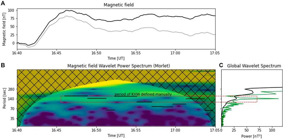
FIGURE 11. Wavelet transform analysis of the geomagnetic field oscillations at Arctic Village, Alaska (ARC) for the E-component, nT, between 1640 and 1705 UT: (A) original (black) series and inverse wavelet transform (gray), each relative to their respective values at 1640 UT; (B) the normalized wavelet power spectrum and shaded COI and (C) the global wavelet for periods outside of the COI (black) and Fourier power spectra (green). Note that the period scale is logarithmic. The horizontal lines in panel (b) indicate periods of KHW defined manually in Figure 3 as the time between dashed lines for corresponding time intervals. The dashed red rectangle corresponds to the period band from 113 to 173 s.
The Lyon-Fedder-Mobarry (LFM) global magnetosphere model, as hosted by the NASA Community Coordinated Modeling Center (CCMC), was used to further investigate the magnetopause configuration in the vicinity of the Cluster spacecraft during the event time frame. The LFM model solves the ideal magnetohydrodynamic (MHD) equations to simulate the 3D interaction between the solar wind and the Earth’s magnetosphere. Further description of the simulation code and its numerical methods can be found in Lyon et al. [54] and Merkin and Lyon [55]. The LFM model can effectively resolve the KHI due to its low diffusion numerical scheme and has been used in previous studies of the KHI [56,57].
The simulation was driven by measured solar wind parameters provided by the virtual OMNI database King and Papitashvili [58] including plasma density, velocities, IMF vector and dipole tilt angle. The simulation was run from 1,600 to 1,730 UT and snapshots of its development at 1,650 and 1657 UT are shown in Figure 12. The background color represents plasma density and the arrows show the velocity vectors. The triangles show the actual location of the four Cluster spacecraft during the event. From the figure, it can be seen that the lower density magnetosphere (dark blue) has developed rolled-up waves at the border with the higher density magnetosheath (light blue). At both times the KH waves are not clearly visible on the dusk side. This is because the horizontal component of the IMF for this event is in the Parker Spiral orientation, making the dusk flank downstream of the quasi-perpendicular bow shock, where the stronger magnetic tension can stabilize the KHI. This is consistent with previous simulation studies of the KHI during Parker Spiral IMF [59] and observations from 6°years of THEMIS data [8].
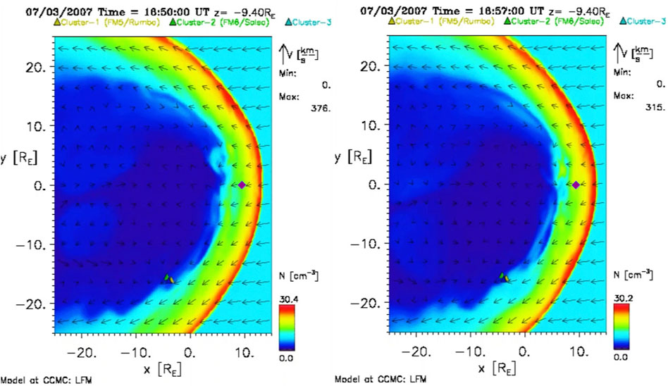
FIGURE 12. Snapshot of the Global MHD (LFM-model) simulation in Solar Magnetic coordinates, driven with solar wind dynamic pressure variations, in the XY-plane with Z = −9.4 RE (solar magnetic coordinates) for July 3, 2007 at 1650 (on the left) and 1657 UT (on the right). Colors represent plasma density (see color bar), arrows represent plasma velocity, and the triangles show the location of the four Cluster spacecraft. The purple diamond denotes the approximate (X, Y) location of the THEMIS-E spacecraft (with ZGSE ≈ −2.4 RE).
Figure 13 displays the simulation driven for constant solar wind and IMF conditions but without any solar wind dynamic pressure variations in order to check whether the ULF waves were caused by pressure driven surface waves or by KHI driven waves. Because the waves were formed in the simulation without any solar wind fluctuations, the non-linear waves seen by Cluster were most likely generated by the KHI. Note that for the unstable boundary conditions, the KHI can be seeded by any perturbation such as magnetic fluctuations [25], velocity fluctuations [60], pressure fluctuations, or any combination of these. The magnitude and frequency of the perturbation can affect the non-linear stage of the instability [60]. Based on the present simulation, the source region for the KHI appears to be on the dayside magnetopause where the magnetosheath flow first diverges dawnward. Note that this is a cut at Z = −9.4 RE and low latitude reconnection is also likely to operate which can act as a seed perturbation for the KHI [25].
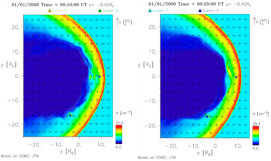
FIGURE 13. Snapshot of the Global MHD (LFM-model) simulation in Solar Magnetic coordinates, driven with constant IMF orientation and without solar wind dynamic pressure variations, in the XY-plane with Z = −9.4 RE (solar magnetic coordinates) for conditions characteristic of July 3, 2007 between 1600 and 1730 UT. The figure on the left shows a snapshot taken at 10 min into the simulation, and the figure on the right shows a snapshot taken at 20 min. Colors represent plasma density (see color bar), arrows represent plasma velocity, and the triangles show the location of the four Cluster spacecraft. The purple diamond denotes the approximate (X, Y) location of the THEMIS-E spacecraft (with ZGSE ≈ −2.4 RE).
All the simulation results and more details on the settings of both runs can be found at https://ccmc.gsfc.nasa.gov/with run-name Katariina_Nykyri_111218_1 (real solar wind and IMF based run) and Katariina_Nykyri_070119_8 (synthetic run without solar wind dynamic pressure variations). A movie of the simulation can be found in the Supplementary Materials, S3. More detailed high-resolution 3D MHD simulations with test particles and Cluster data comparison is left for our future work.
Based on the Cluster observations, the Pc4 event shown here can be interpreted as the KHI because:
1) The magnetic field magnitude and normal component maxima were aligned with the pressure maxima, indicating that the spacecraft were traversing the rolled-up KHWs [5,17]. This differs from instances of observing either FTEs or persistent surface waves. In the case of FTE observation, the pressure maxima is expected at its core (the center of the bipolar BN) and the bipolar BN fluctuations are separated by repetitious quiet periods with periods longer than 4 min [6]. In the case of persistent surface waves, the pressure maxima would be associated with the bipolar BN = 0 crossings. These KHW magnetic field and total pressure signatures occurred in conjunction with periodical observations of magnetospheric and magnetosheath plasma populations (jumps in the density at the hyperbolic points), indicating that the KHI had developed into the vortices necessary for energy transport across the magnetopause [61];
2) VM and VN and BM and BN are mainly in anti-phase, indicating that there are vortex formations according to Yan et al. [33]. In the case of FTEs, the velocity components will not show such anti-phase behavior;
3) The angle between the average boundary normal and the boundary normals, calculated for subsequent 1 min windows centered on each point in the time series, oscillates between opposite directions;
4) The HT velocity vectors show oscillations at the boundary region;
5) Fast-moving, low-density plasma populations associated with the mixing of two plasma environments are observed;
6) Pc4 is a typical KHW frequency.
The interpretation of the observations is also supported by the global modeling. The rolled-up vortices were clearly seen in LFM simulation results for the event, confirming that the solar wind conditions were favorable for KHW development. The favorable solar wind conditions are also supported by the analysis of the magnetopause shear angle. It has been shown that when the IMF has a strong Parker spiral component, the KHI can develop with tilted k-vectors with respect to the shear flow plane to maximize the onset condition [8,41,62], which could explain why KHWs were observed by Cluster at high latitudes.
Several of the KHI vortices observed in this event were likely accompanied by reconnection events as indicated by the Walén relation, the presence of deHoffmann-Teller frames, field-aligned ion beams observed together with bipolar fluctuations in the normal magnetic field component, and crescent distributions. The relation between the KHI and reconnection is highly dependent upon the magnetic field direction with respect to the sheared flow.
For northward IMF conditions, Otto and Fairfield [3] demonstrated that as long as there is a KH wave vector component along the magnetic field, the nonlinear KH mode can twist the magnetic field line and consequently generate a strong anti-parallel component. This then triggers magnetic reconnection (even without an anti-parallel magnetic component in the initial condition). Later, Nakamura et al. [63] showed that if there is an anti-parallel magnetic component across the sheared flow, the spin region (trailing edge) of the KH wave can thin the current sheet, which also triggers magnetic reconnection. The above two KH driven reconnection mechanisms are described in a two-dimensional perspective. In three-dimensions, the KHI can strongly twist magnetic field lines in its active region, which triggers a pair of middle-latitude component reconnections (e.g., [64–66]).
For the southward IMF condition, as is namely the case in this paper according to the OMNI data and THEMIS observations at the subsolar point, there are pre-existing anti-parallel magnetic field components (mainly along the north-south direction) that are mostly perpendicular to the sheared flow (mainly along the Sun-Earth direction). This configuration is unstable for both magnetic reconnection and KHI. Thus, both KHI (mostly in XYGSE plane) and reconnection (mostly in XZGSE plane) can operate simultaneously [23], One process can be initialized earlier or grow faster than the other. But it does not have to be that one triggers another. The onset of KHI can locally thin the current sheet which triggers reconnection, especially in the spine region (trailing edge) (see illustration of such coupling in Figures 4, 6, 11 (at t = 124 s) in Ma et al. [24]). Note that the majority of open flux are connected through the spine region. In the vicinity of vortices, plasma flow strongly twists magnetic field lines which generates patchy reconnection and complex flux rope structures. Both strongly anti-parallel magnetic field and reconnection jets (i.e., along the Z-direction), may not be easily observed (see also [67]). In our study we observe field-aligned beams together with bipolar BN magnetic field fluctuations as an indication of reconnection. The onset of magnetic reconnection can change the width of the sheared flow, and consequently changes the KH wavelength [25]. This event demonstrates the complexity of the instabilities generated at the magnetopause.
Source regions for longer wavelengths and lower frequencies are expected farther down the magnetotail. For the present KHI associated with reconnection event, there are three possible source regions. The first is close to the subsolar point where magnetosheath flow first starts to diverge and where KHI growth may be enhanced by both dayside reconnection [25] and by solar wind velocity and pressure fluctuations [60]. The latter enhancement was also demonstrated by the LFM simulation of this event. The second source region is at the dawn sector of the southern cusp [68], and the third region is farther down the tail where flow from tail reconnection is moving Earthward and forms a shear layer. This velocity shear layer is observable in the LFM simulation, see, e.g., Figure 12. Most relevant for the present event are the first two source regions, and future work will need to address the possible KHI associated with reconnection interference from multiple sources.
ULF waves in the magnetosphere have been correlated with solar wind conditions. For example, dynamic pressure variations are known to generate pulsations [69]. However, the solar wind speed, IMF magnitude, Alfvénic Mach number (not shown), and flow dynamic pressure from the OMNI data all remained nearly constant during the event, ruling out the likelihood of the ULF waves observed by Cluster being driven directly by pressure perturbations.
There were solar wind ion pressure pulsations preceding the event which may have acted as seed perturbations at the subsolar point, providing for the propagation and development of the event KHWs seen farther down the flank [70]. In fact, three of the THEMIS spacecraft situated in the magnetosheath at the subsolar point during this event recorded signatures of significant boundary motion, including pressure perturbations, which further supports this hypothesis. Figure 14 shows the pressure tensor for the xx −, yy −, and zz − components (red, blue, green, respectively) recorded by the Electrostatic Analyzer (ESA) onboard THEMIS-E (P4). The ion pressure moment data were obtained from reduced-mode data, which has a degraded angular resolution, but high time resolution (∼ 3 s). Similar plots for THEMIS-C and THEMIS-D can be found in the Supplementary Materials, see Supplementary Figures S4, S5.
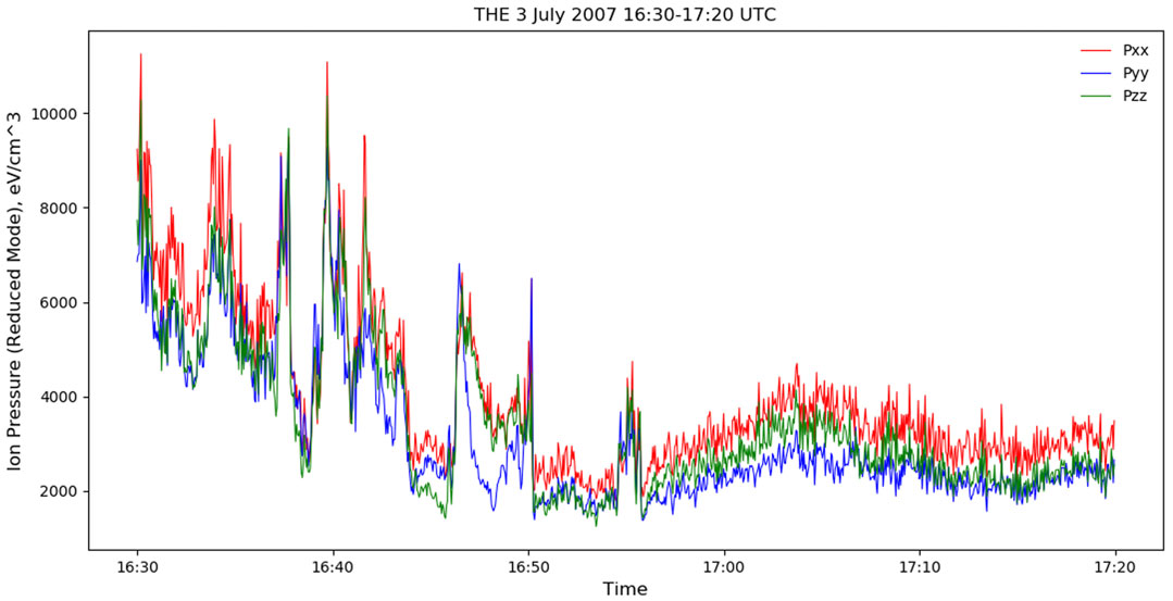
FIGURE 14. THEMIS-E pressure tensor for the xx − (red), yy − (blue), and zz − components (green), eV cm−3, recorded by the Electrostatic Analyzer (ESA). Reduced mode data are shown for July 3, 2007 from 1630 to 1720 UT.
We did the wavelet analysis of the magnetic field BZ,GSE fluctuations observed by THEMIS-E, see Figure 15. We do observe spikes of the wave power at the periods of 140 and 70 s which is in agreement with the spikes observed by Cluster. Therefore, these fluctuations (via reconnection) may have further modulated the KHWs.
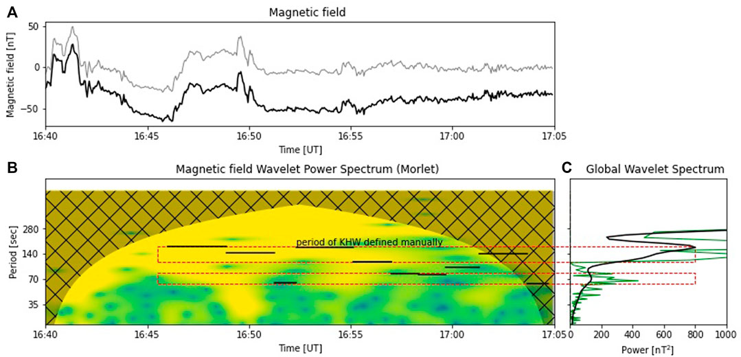
FIGURE 15. Wavelet transform analysis of the magnetic field oscillations for the ZGSE-component, nT, observed by THEMIS-E between 1640 and 1705 UT: (A) original (black) series and inverse (gray) wavelet transform; (B) the normalized wavelet power spectrum and shaded cone of influence and (C) the global wavelet for periods outside of the COI (black) and Fourier power spectra (green). Note that the period scale is logarithmic. The horizontal lines in panel (b) indicate periods of KHW defined manually in Figure 3 as the time between dashed lines for corresponding time intervals. The dashed red rectangles correspond to two period bands from 62 to 82 s and from 113 to 173 s.
THEMIS-E also observes magnetosheath jets (see the plasma ram pressure pulsations in Supplementary Figure S6 in the Supplementary Materials) with a periodicity of about 5 min, which would result in dayside magnetopause oscillations and/or magnetopause reconnection [71,72], and possibly also modulate the KHWs and associated reconnection. The origin and dynamics of these jets is beyond the scope of this paper and is left for a future study.
The current debate surrounding the extent of magnetospheric effects caused by KHWs at the magnetopause remains an exciting topic as more and more in situ observations become available for analysis. This process’ role in the generation of ULF waves at the Earth’s ground, in particular, continues to be uncertain since different potential drivers have been identified. The event scrutinized in this article suggests a relation between the KHI associated with reconnection and ground-based ULF waves.
On July 3, 2007 Cluster encountered KHWs at the high-latitude magnetopause. Signatures of these waves included bipolar fluctuations in the magnetic field normal component at the edge of total pressure maxima mostly coinciding with alternations of the low-density, low-speed and high-energy magnetospheric plasma with the high-density, high-speed, and low-energy magnetosheath plasma; existence of fast-moving, low-density mixed plasma; quasi-periodic oscillations of the boundary normal; and the boundary normal and parallel velocity components being in anti-phase. The KHWs exhibited frequency peaks in the Pc4 range which is typical for this instability. Several of the observed KHI vortices were accompanied by reconnection as indicated by the Walén relation, the presence of deHoffmann-Teller frames, field-aligned ion beams observed together with bipolar fluctuations in the normal magnetic field component, and crescent distributions. LFM simulations of the observed event conditions also resulted in KHWs at the magnetopause.
During the same time as the event at the magnetopause, there were Pc4 ULF perturbations recorded at ground-based geomagnetic stations. These pulsations were observed around the location of the foot point corresponding to the field line of the location of the spacecraft recordings. Solar wind conditions during the event were rather steady. The solar wind speed was low and the IMF magnitude was nearly constant. Only minimal pressure perturbations were recorded and the BZ component of the IMF, according to the OMNI data, remained southward without strong fluctuations. However, the fluctuations in the southward IMF and plasma/ram pressure at the subsolar point may have triggered KHWs.
The conditions recorded during this case study provide evidence for the likelihood that Pc4 ULF waves can be generated by the KHI associated with reconnection at the magnetopause. This suggests that the KHI can play a role in the transfer of energy from the solar wind to the magnetosphere. However, further studies are needed before the ubiquity of such an event can be declared.
The datasets presented in this study can be found in online repositories. The names of the repository/repositories and accession number(s) can be found below: The Cluster data can be found in the Cluster Science Archive (https://csa.esac.esa.int). The SuperMAG data can be found at http://supermag.jhuapl.edu. We also used NASA/GSFC’s Space Physics Data Facility’s OMNIWeb (or CDAWeb or ftp - see https://cdaweb.sci.gsfc.nasa.gov/index.html) service, and OMNI data (https://omniweb.gsfc.nasa.gov). Data from the THEMIS Mission can be found at http://themis.igpp.ucla.edu/index.shtml). The results presented in this paper rely on the data collected at the Arctic Village and Kaktovik magnetometers, provided by the Geophysical Institute Magnetometer Array operated by the Geophysical Institute, University of Alaska (https://www.gi.alaska.edu/monitors/magnetometer/archive). Global LFM MHD simulations have been provided by the Community Coordinated Modeling Center at Goddard Space Flight Center through their public runs on request system (http://ccmc.gsfc.nasa.gov).
EK led the manuscript, did data analysis, produced figures, contributed to the text and wrote the Volkswagen proposal. JGo led the manuscript, did data analysis, produced figures and contributed to the text. KN led the MHD simulations, did data analysis, produced figures and contributed to the text. AS produced figures and contributed to the text. JGj and MF provided SuperMAG data and assisted in its use. EG did data analysis, produced a figure, contributed to the text and wrote the Volkswagen proposal. LK and KT produced figures. XM contributed to a figure and the text.
The work of JG, EG, LK, and EK is supported by the Volkswagen Foundation under grant Az 90 312, Az 90 312-1 and Az 97 742. Work by KN and XM is supported by the NASA grant ##NNX17AI50G. The work of EK is also supported by German Research Foundation (DFG) under number KR 4375/2-1 within SPP “Dynamic Earth”.
The authors declare that the research was conducted in the absence of any commercial or financial relationships that could be construed as a potential conflict of interest.
All claims expressed in this article are solely those of the authors and do not necessarily represent those of their affiliated organizations, or those of the publisher, the editors and the reviewers. Any product that may be evaluated in this article, or claim that may be made by its manufacturer, is not guaranteed or endorsed by the publisher.
The authors would like to thank the Cluster Science Archive team for providing the data and assistance in obtaining the CIS plot. We acknowledge NASA contract NAS5-02099 and V. Angelopoulos for use of data from the THEMIS Mission, specifically, C. W. Carlson and J. P. McFadden for use of ESA data.
The Supplementary Material for this article can be found online at: https://www.frontiersin.org/articles/10.3389/fphy.2021.738988/full#supplementary-material
1The observation of closed magnetic field lines is indicated by the energy of maxima intensity in spectrograms of Figure 1, which is significantly higher than those typical for the plasma mantle,
1. Southwood DJ. Some Features of Field Line Resonances in the Magnetosphere. Planet Space Sci (1974) 22:483–91. doi:10.1016/0032-0633(74)90078-6
2. Fairfield DH, Otto A, Mukai T, Kokubun S, Lepping RP, Steinberg JT, et al. Geotail Observations of the Kelvin-Helmholtz Instability at the Equatorial Magnetotail Boundary for Parallel Northward fields. J Geophys Res (2000) 105:21159–73. doi:10.1029/1999ja000316
3. Otto A, Fairfield DH. Kelvin-Helmholtz Instability at the Magnetotail Boundary: MHD Simulation and Comparison with Geotail Observations. J Geophys Res (2000) 105:21175–90. doi:10.1029/1999ja000312
4. Nykyri K, Otto A. Plasma Transport at the Magnetospheric Boundary Due to Reconnection in Kelvin-Helmholtz Vortices. Geophys Res Lett (2001) 28:3565–8. doi:10.1029/2001gl013239
5. Hasegawa H, Fujimoto M, Phan T-D, Rème H, Balogh A, Dunlop MW, et al. Transport of Solar Wind into Earth's Magnetosphere through Rolled-Up Kelvin-Helmholtz Vortices. Nature (2004) 430:755–8. doi:10.1038/nature02799
6. Kavosi S, Raeder J. Ubiquity of Kelvin-Helmholtz Waves at Earth's Magnetopause. Nat Commun (2015) 6. doi:10.1038/ncomms8019
7. Yu Y, Ridley AJ. Exploring the Influence of Ionospheric O+ Outflow on Magnetospheric Dynamics: The Effect of Outflow Intensity. J Geophys Res Space Phys (2013) 118:5522–31. doi:10.1002/jgra.50528
8. Henry ZW, Nykyri K, Moore TW, Dimmock AP, Ma X. On the Dawn-Dusk Asymmetry of the Kelvin-Helmholtz Instability between 2007 and 2013. J Geophys Res Space Phys (2017) 122:888–11. doi:10.1002/2017JA024548
9. Hasegawa A, Chen L. Theory of Magnetic Pulsations. Space Sci Rev (1974) 16:347–59. doi:10.1007/bf00171563
10. Nykyri K, Dimmock AP. Statistical Study of the ULF Pc4-Pc5 Range Fluctuations in the Vicinity of Earth's Magnetopause and Correlation with the Low Latitude Boundary Layer Thickness. Adv Space Res (2016) 58:257–67. doi:10.1016/j.asr.2015.12.046
11. Wing S, Johnson JR, Newell PT, Meng C-I. Dawn-dusk Asymmetries, Ion Spectra, and Sources in the Northward Interplanetary Magnetic Field Plasma Sheet. J Geophys Res (2005) 110. doi:10.1029/2005JA011086
12. Moore TW, Nykyri K, Dimmock AP. Ion‐Scale Wave Properties and Enhanced Ion Heating across the Low‐Latitude Boundary Layer during Kelvin‐Helmholtz Instability. J Geophys Res Space Phys (2017) 122:11128–11153. doi:10.1002/2017JA024591
13. Dimmock AP, Nykyri K. The Statistical Mapping of Magnetosheath Plasma Properties Based on THEMIS Measurements in the Magnetosheath Interplanetary Medium Reference Frame. J Geophys Res Space Phys (2013) 118:4963–76. doi:10.1002/jgra.50465
14. Lotko W, Streltsov AV, Carlson CW. Discrete Auroral Arc, Electrostatic Shock and Suprathermal Electrons Powered by Dispersive, Anomalously Resistive Field Line Resonance. Geophys Res Lett (1998) 25:4449–52. doi:10.1029/1998gl900200
15. Elkington SR, Hudson MK, Chan AA. Resonant Acceleration and Diffusion of Outer Zone Electrons in an Asymmetric Geomagnetic Field. J Geophys Res (2003) 108. doi:10.1029/2001JA009202
16. Kronberg EA, Grigorenko EE, Turner DL, Daly PW, Khotyaintsev Y, Kozak L. Comparing and Contrasting Dispersionless Injections at Geosynchronous Orbit during a Substorm Event. J Geophys Res Space Phys (2017) 122:3055–72. doi:10.1002/2016JA023551
17. Hasegawa H. Structure and Dynamics of the Magnetopause and its Boundary Layers. Monogr Environ Earth Planets (2012) 1:71–119. doi:10.5047/meep.2012.00102.0071
18. Bentley SN, Watt CEJ, Owens MJ, Rae IJ. ULF Wave Activity in the Magnetosphere: Resolving Solar Wind Interdependencies to Identify Driving Mechanisms. J Geophys Res Space Phys (2018) 123:2745–71. doi:10.1002/2017JA024740
19. Rae IJ, Donovan EF, Mann IR, Fenrich FR, Watt CEJ, Milling DK, et al. Evolution and Characteristics of Global Pc5 ULF Waves during a High Solar Wind Speed Interval. J Geophys Res (2005) 110. doi:10.1029/2005JA011007
20. Agapitov O, Glassmeier K-H, Plaschke F, Auster H-U, Constantinescu D, Angelopoulos V, et al. Surface Waves and Field Line Resonances: A Themis Case Study. J Geophys Res (2009) 114:a–n. doi:10.1029/2008JA013553
21. Walker ADM. The Kelvin-Helmholtz Instability in the Low-Latitude Boundary Layer. Planet Space Sci (1981) 29:1119–33. doi:10.1016/0032-0633(81)90011-8
22. Dougal ER, Nykyri K, Moore TW. Mapping of the Quasi-Periodic Oscillations at the Flank Magnetopause into the Ionosphere. Ann Geophys (2013) 31:1993–2011. doi:10.5194/angeo-31-1993-2013
23. Wang CP, Thorne R, Liu TZ, Hartinger MD, Nagai T, Angelopoulos V, et al. A Multispacecraft Event Study of Pc5 Ultralow‐frequency Waves in the Magnetosphere and Their External Drivers. J Geophys Res Space Phys (2017) 122:5132–47. doi:10.1002/2016JA023610
24. Ma X, Otto A, Delamere PA. Interaction of Magnetic Reconnection and Kelvin-Helmholtz Modes for Large Magnetic Shear: 1. Kelvin-Helmholtz Trigger. J Geophys Res Space Phys (2014) 119:781–97. doi:10.1002/2013JA019224
25. Ma X, Otto A, Delamere PA. Interaction of Magnetic Reconnection and Kelvin-Helmholtz Modes for Large Magnetic Shear: 2. Reconnection Trigger. J Geophys Res Space Phys (2014) 119:808–20. doi:10.1002/2013JA019225
26. Kronberg EA, Gastaldello F, Haaland S, Smirnov A, Berrendorf M, Ghizzardi S, et al. Prediction and Understanding of Soft-Proton Contamination in XMM-Newton: A Machine Learning Approach. ApJ (2020) 903:89. doi:10.3847/1538-4357/abbb8f
27. Laakso H, Perry C, McCaffrey S, Herment D, Allen AJ, Harvey CC, et al. Cluster Active Archive: Overview. Cluster Active Archive: Overview. (2010). p. 3–37. doi:10.1007/978-90-481-3499-1_1
28. Rème H, Aoustin C, Bosqued JM, Dandouras I, Sauvaud JA, Barthe A, et al. First Multispacecraft Ion Measurements in and Near the Earth’ S Magnetosphere with the Identical Cluster Ion Spectrometry (CIS) experiment. Ann Geophysicae (2001) 19:1303–54. doi:10.5194/angeo-19-1303-2001
29. Balogh A, Carr CM, Acuña MH, Dunlop MW, Beek TJ, Brown P, et al. The Cluster Magnetic Field Investigation: Overview of In-Flight Performance and Initial Results. Ann Geophys (2001) 19:1207–17. doi:10.5194/angeo-19-1207-2001
30. Escoubet CP, Schmidt R, Goldstein ML. Cluster—Science and mission Overview. Space Sci Rev (1997) 79:11–32. doi:10.1023/a:1004923124586
31. Siscoe GL, Davis L, Coleman PJ, Jones DE, Jones DE. Power Spectra and Discontinuities of the Interplanetary Magnetic Field: Mariner 4. J Geophys Res (1968) 73:61–82. doi:10.1029/JA073i001p00061
32. Dunlop MW, Woodward TI, Farrugia CJ. Minimum Variance Analysis: Cluster Themes. In: KH Glassmeier, U Motschmann, and R Schmidt, editors. Proceedings of the Cluster Workshops, Data Analysis Tools and Physical Measurements and Mission-Oriented Theory, 371. Paris: ESA Special Publication (1995). p. 33.
33. Yan GQ, Mozer FS, Shen C, Chen T, Parks GK, Cai CL, et al. Kelvin-Helmholtz Vortices Observed by THEMIS at the Duskside of the Magnetopause under Southward Interplanetary Magnetic Field. Geophys Res Lett (2014) 41:4427–34. doi:10.1002/2014GL060589
34. Miura A. Self-Organization in the Two-Dimensional Kelvin-Helmholtz Instability. Phys Rev Lett (1999) 83:1586–9. doi:10.1103/PhysRevLett.83.1586
35. Sonnerup BUÖ, Paschmann G, Phan T-D Fluid Aspects of Reconnection at the Magnetopause: In Situ Observations, 90. Washington DC. American Geophysical Union Geophysical Monograph Series (1995). p. 167–80. doi:10.1029/GM090p0167
36. Hasegawa H, Fujimoto M, Takagi K, Saito Y, Mukai T, Rème H. Single-spacecraft Detection of Rolled-Up Kelvin-Helmholtz Vortices at the Flank Magnetopause. J Geophys Res (2006) 111. doi:10.1029/2006JA011728
37. Taylor MGGT, Hasegawa H, Lavraud B, Phan T, Escoubet CP, Dunlop MW, et al. Spatial Distribution of Rolled up Kelvin-Helmholtz Vortices at Earth's Dayside and Flank Magnetopause. Ann Geophys (2012) 30:1025–35. doi:10.5194/angeo-30-1025-2012
38. Johnson JR, Wing S. Northward Interplanetary Magnetic Field Plasma Sheet Entropies. J Geophys Res (2009) 114:a–n. doi:10.1029/2008JA014017
39. Jacobs JA, Kato Y, Matsushita S, Troitskaya VA. Classification of Geomagnetic Micropulsations. J Geophys Res (1964) 69:180–1. doi:10.1029/JZ069i001p00180
40. Paschmann G, Haaland S, Sonnerup BUÖ, Hasegawa H, Georgescu E, Klecker B, et al. Characteristics of the Near-Tail Dawn Magnetopause and Boundary Layer. Ann Geophys (2005) 23:1481–97. doi:10.5194/angeo-23-1481-2005
41. Nykyri K, Otto A, Lavraud B, Mouikis C, Kistler LM, Balogh A, et al. Cluster Observations of Reconnection Due to the Kelvin-Helmholtz Instability at the Dawnside Magnetospheric Flank. Ann Geophys (2006) 24:2619–43. doi:10.5194/angeo-24-2619-2006
42. Torbert RB, Burch JL, Phan TD, Hesse M, Argall MR, Shuster J, et al. Electron-scale Dynamics of the Diffusion Region during Symmetric Magnetic Reconnection in Space. Science (2018) 362:1391–5. doi:10.1126/science.aat2998
43. Gjerloev JW. The SuperMAG Data Processing Technique. J Geophys Res (2012) 117:a–n. doi:10.1029/2012JA017683
44. Tsyganenko NA. A Magnetospheric Magnetic Field Model with a Warped Tail Current Sheet. Planet Space Sci (1989) 37:5–20. doi:10.1016/0032-0633(89)90066-4
45. Boscher D, Bourdarie S, O’Brien P, Guild T. Irbem-lib Library. (2012). Availableat: https://github.com/PRBEM (Accessed June 1, 2021).
46. Shumko M, Sample J, Johnson A, Blake B, Crew A, Spence H, et al. Microburst Scale Size Derived from Multiple Bounces of a Microburst Simultaneously Observed with the FIREBIRD-II CubeSats. Geophys Res Lett (2018) 45:8811–8. doi:10.1029/2018GL078925
47. Dunlop MW, Yang JY, Yang YY, Xiong C, Lühr H, Bogdanova YV, et al. Simultaneous Field‐aligned Currents at Swarm and Cluster Satellites. Geophys Res Lett (2015) 42:3683–91. doi:10.1002/2015GL063738
48. Tsyganenko NA, Stern DP. Modeling the Global Magnetic Field of the Large-Scale Birkeland Current Systems. J Geophys Res (1996) 101:27187–98. doi:10.1029/96JA02735
49. Trattner KJ, Mulcock JS, Petrinec SM, Fuselier SA. Probing the Boundary between Anti-parallel and Component Reconnection during Southwards Interplanetary Magnetic Field Conditions. J Geophys Res (2007) 112. doi:10.1029/2007ja012270
50. Trattner KJ, Burch JL, Ergun R, Eriksson S, Fuselier SA, Giles BL, et al. The MMS Dayside Magnetic Reconnection Locations during Phase 1 and Their Relation to the Predictions of the Maximum Magnetic Shear Model. J Geophys Res Space Phys (2017) 122:991–12. doi:10.1002/2017JA024488
51. Hughes WJ, Southwood DJ. The Screening of Micropulsation Signals by the Atmosphere and Ionosphere. J Geophys Res (1976) 81:3234–40. doi:10.1029/JA081i019p03234
52. Sciffer MD, Waters CL. Propagation of ULF Waves through the Ionosphere: Analytic Solutions for Oblique Magnetic fields. J Geophys Res (2002) 107:1297. doi:10.1029/2001JA000184
53. Paschmann G, Haaland S, Treumann R. Auroral Plasma Physics. Space Sci Rev (2002) 103. doi:10.1023/A:1023030716698
54. Lyon JG, Fedder JA, Mobarry CM. The Lyon-Fedder-Mobarry (LFM) Global MHD Magnetospheric Simulation Code. J Atmos Solar-Terrestrial Phys (2004) 66. doi:10.1016/j.jastp.2004.03.020
55. Merkin VG, Lyon JG. Effects of the Low-Latitude Ionospheric Boundary Condition on the Global Magnetosphere. J Geophys Res (2010) 115:a–n. doi:10.1029/2010JA015461
56. Merkin VG, Lyon JG, Claudepierre SG. Kelvin-Helmholtz Instability of the Magnetospheric Boundary in a Three-Dimensional Global MHD Simulation during Northward IMF Conditions. J Geophys Res Space Phys (2013) 118:5478–96. doi:10.1002/jgra.50520
57. Sorathia KA, Merkin VG, Ukhorskiy AY, Allen RC, Nykyri K, Wing S. Solar Wind Ion Entry into the Magnetosphere during Northward IMF. J Geophys Res Space Phys (2019) 124:5461–81. doi:10.1029/2019JA026728
58. King JH, Papitashvili NE. Solar Wind Spatial Scales in and Comparisons of Hourly Wind and ACE Plasma and Magnetic Field Data. J Geophys Res (2005) 110. doi:10.1029/2004JA010649
59. Nykyri K. Impact of MHD Shock Physics on Magnetosheath Asymmetry and Kelvin-Helmholtz Instability. J Geophys Res Space Phys (2013) 118:5068–81. doi:10.1002/jgra.50499
60. Nykyri K, Ma X, Dimmock A, Foullon C, Otto A, Osmane A. Influence of Velocity Fluctuations on the Kelvin-Helmholtz Instability and its Associated Mass Transport. J Geophys Res Space Phys (2017) 122:9489–512. doi:10.1002/2017JA024374
61. Moore TW, Nykyri K, Dimmock AP. Cross-scale Energy Transport in Space Plasmas. Nat Phys (2016) 12:1164–9. doi:10.1038/NPHYS3869
62. Adamson E, Nykyri K, Otto A. The Kelvin-Helmholtz Instability under Parker-spiral Interplanetary Magnetic Field Conditions at the Magnetospheric Flanks. Adv Space Res (2016) 58:218–30. doi:10.1016/j.asr.2015.09.013
63. Nakamura TKM, Fujimoto M, Otto A. Magnetic Reconnection Induced by Weak Kelvin-Helmholtz Instability and the Formation of the Low-Latitude Boundary Layer. Geophys Res Lett (2006) 33:L14106. doi:10.1029/2006GL026318
64. Otto A. Mass Transport at the Magnetospheric Flanks Associated with Three-Dimensional Kelvin- Helmholtz Modes. AGU Fall Meeting Abstracts, 2006 (2006). p. SM33B–0365.
65. Faganello M, Califano F, Pegoraro F, Andreussi T. Double Mid-latitude Dynamical Reconnection at the Magnetopause: An Efficient Mechanism Allowing Solar Wind to Enter the Earth's Magnetosphere. Epl (2012) 100:69001. doi:10.1209/0295-5075/100/69001
66. Ma X, Delamere P, Otto A, Burkholder B. Plasma Transport Driven by the Three‐Dimensional Kelvin‐Helmholtz Instability. J Geophys Res Space Phys (2017) 122:10382. doi:10.1002/2017JA024394
67. Hwang K-J, Kuznetsova MM, Sahraoui F, Goldstein ML, Lee E, Parks GK. Kelvin-Helmholtz Waves under Southward Interplanetary Magnetic Field. J Geophys Res (2011) 116:a–n. doi:10.1029/2011JA016596
68. Nykyri K, Ma X, Burkholder B, Rice R, Johnson JR, Kim EK, et al. MMS Observations of the Multiscale Wave Structures and Parallel Electron Heating in the Vicinity of the Southern Exterior Cusp. J Geophys Res Space Phys (2021) 126:e27698. doi:10.1029/2019JA027698
69. Hwang K-J, Sibeck DG. Role of Low-Frequency Boundary Waves in the Dynamics of the Dayside Magnetopause and the Inner Magnetosphere. Hoboken, NJ: John Wiley (2016). p. 213–39. doi:10.1002/9781119055006.ch13
70. Hartinger MD, Plaschke F, Archer MO, Welling DT, Moldwin MB, Ridley A. The Global Structure and Time Evolution of Dayside Magnetopause Surface Eigenmodes. Geophys Res Lett (2015) 42:2594–602. doi:10.1002/2015GL063623
71. Hietala H, Phan TD, Angelopoulos V, Oieroset M, Archer MO, Karlsson T, Karlsson T, et al. In Situ Observations of a Magnetosheath High-Speed Jet Triggering Magnetopause Reconnection. Geophys Res Lett (2018) 45:1732–40. doi:10.1002/2017GL076525
72. Nykyri K, Bengtson M, Angelopoulos V, Nishimura Y, Wing S. Can Enhanced Flux Loading by High‐Speed Jets Lead to a Substorm? Multipoint Detection of the Christmas Day Substorm Onset at 08:17 UT, 2015. J Geophys Res Space Phys (2019) 124:4314–40. doi:10.1029/2018JA026357
73. Wang C-P, Lyons LR, Angelopoulos V. Properties of Low-Latitude Mantle Plasma in the Earth's Magnetotail: ARTEMIS Observations and Global MHD Predictions. J Geophys Res Space Phys (2014) 119:7264–80. doi:10.1002/2014JA020060
Keywords: kelvin-helmholtz instability, reconnection, magnetosheath, magnetopause, ULF waves at the ground, global magnetohydrodynamic simulation
Citation: Kronberg EA, Gorman J, Nykyri K, Smirnov AG, Gjerloev JW, Grigorenko EE, Kozak LV, Ma X, Trattner KJ and Friel M (2021) Kelvin-Helmholtz Instability Associated With Reconnection and Ultra Low Frequency Waves at the Ground: A Case Study. Front. Phys. 9:738988. doi: 10.3389/fphy.2021.738988
Received: 09 July 2021; Accepted: 05 November 2021;
Published: 02 December 2021.
Edited by:
Xochitl Blanco-Cano, National Autonomous University of Mexico, MexicoReviewed by:
Binbin Tang, National Space Science Center (CAS), ChinaCopyright © 2021 Kronberg, Gorman, Nykyri, Smirnov, Gjerloev, Grigorenko, Kozak, Ma, Trattner and Friel. This is an open-access article distributed under the terms of the Creative Commons Attribution License (CC BY). The use, distribution or reproduction in other forums is permitted, provided the original author(s) and the copyright owner(s) are credited and that the original publication in this journal is cited, in accordance with accepted academic practice. No use, distribution or reproduction is permitted which does not comply with these terms.
*Correspondence: E. A. Kronberg , a3JvbmJlcmdAZ2VvcGh5c2lrLnVuaS1tdWVuY2hlbi5kZQ==
Disclaimer: All claims expressed in this article are solely those of the authors and do not necessarily represent those of their affiliated organizations, or those of the publisher, the editors and the reviewers. Any product that may be evaluated in this article or claim that may be made by its manufacturer is not guaranteed or endorsed by the publisher.
Research integrity at Frontiers
Learn more about the work of our research integrity team to safeguard the quality of each article we publish.