Numerical Simulation of Thermal Field in Mass Concrete With Pipe Water Cooling

Water pipe cooling is mainly used to control temperature in the construction of mass concrete structures. It is important to reveal how to accurately stimulate the temperature field of mass concrete under action of this water pipe cooling. This paper presents a new method for this purpose. In this method, the contact surface of the water pipe and the concrete is used as the heat dissipation surface into the control equation and the composite Multiquadrics radial basis function (MQ-RBF) and low-order linear polynomial combination are used to discrete the spatial domain. The heat dissipation surface of the water pipe is included in the boundary conditions so that there is no need to build the refined water pipe modeling. This new method not only reduces the calculation cost but also ensures calculation accuracy. Through four calculation examples, this paper show that the algorithm has advantages in the numerical simulation of the concrete temperature field with water pipe cooling.

Introduction

Mass concrete can release a lot of hydration heat during the construction process, especially in its early stage. In this early stage of concrete construction, a higher temperature is generated through the violent chemical reaction and the poor thermal conductivity. Generally, the highest temperature on the surface of the mass concrete bearing platform is about 30°C, and the highest temperature inside is approximately 50°C. The surface is directly contact with the air to dissipate heat. Thus, the temperature difference between the inside and outside of the concrete becomes larger. As a result, it generates more significant tensile stress. For the safety of the structure, it is necessary to control the concrete temperature in the early stage of construction.

It is very difficult to accurately simulate the temperature field of the concrete around the cooling water pipe. The reason is that it is a typical problem of the heat conduction between circulating fluids and solids in small calibers . The diameter of the water pipe is much smaller than the size of the concrete structure. In addition, the temperature gradient around the water pipe is also large.

There are three main approaches to solving this problem. The first type is the equivalent adiabatic temperature rise method proposed by Zhu [1] to simulate the impact of water pipe cooling. The algorithm principle is to use the cooling water pipe as a heat loss term and to only consider the temperature field in the average sense of concrete. Although this method only needs to draw a simple grid to calculate the temperature field in the cooling influence of the water pipe, the drastic changes in the temperature near the water pipe were ignored. It cannot obtain an accurate temperature field around the water pipe. The second type is named a refine grid algorithm. This algorithm considers the actual existence of water pipes, and the temperature in the boundary surface-contact surface between concrete and water pipers as a known one, and arranges dense grids near the water pipes. It can accurately simulate the temperature gradient near the water pipe by methods of refining the grid, but the calculation and modelling cost is too high to achieve in the actual modelling. In this paper, the solution obtained by the fine grid is called a refined solution. The third type is to construct a special water pipe unit, whose purpose is to reduce the calculation scale and ensure a certain accuracy. Many people put forward different ways to solve this problem. Kim [2] regards water pipes as line elements and uses common nodes to simulate the heat exchange between water pipes and concrete. However, the water pipes in this method can only be arranged on grid nodes, and the calculation uses Lagrange units. In order to obtain accurate solutions, it is necessary to refine the grid around the water pipe. Zuo [3] et al. used an extended finite element method (FEM) to solve the water pipe cooling problem, but at present, he can only simulate the water pipe cooling problem in the two-dimensional state. It is noticeable that he did not give a method for the temperature field simulation in the three-dimensional state. Chen [4] proposed to place the water pipe inside the concrete unit, to set up a “water pipe embedded unit,” and put the contact surface between the water pipe and concrete-the heat dissipation surface-into the governing equation. However, the unit around the water pipe is still linear. To accurately simulate the temperature around the water pipe, a refined mesh is needed.

As the most extensive numerical method in engineering applications and scientific calculations, the FEM has an excellent theoretical foundation and is unquestionable in terms of accuracy, stability, and reliability. With the development of numerical computing in recent years, this meshless method has attracted people’s attention because of its high actuarial accuracy, grid-independence, and adaptive capacity [5, 6], and it has been a very popular research direction. The main meshless methods currently studied contain Element-free Galerkin (EFG) method [7–9] based on moving least squares approximation and, Petrov-Galerkin (MLPG) method [10–13], smooth particles hydrodynamics (SPH) method [14–19] and, regenerated kernel particle method (RKPM) [20–22] based on integral form approximation, and polynomial point interpolation method (PIM) [23] and radial point interpolation method (RPIM) [24–27] based on point interpolation, and various improved methods such as spectral meshless radial point interpolation (SMRPI) [28],etc.

In this paper, a meshless interpolation method based on the global weak-form RPIM is used to simulate the heat exchange process between water pipes and concrete. The RPIM was proposed to solve the singularity problem of the moment matrix in the polynomial PIM. Traditionally, the shape function of PIM was constructed by using a polynomial basis function. This method has a significant advantage in dealing with essential boundary conditions because its shape function has the δ function property. But in the process of calculating the shape function, its moment matrix is very prone to singularity. In order to improve this method, Liu [24] proposed the RPIM. The RPIM solves the problem of matrix singularity by coupling the polynomial basis function with the radial basis function, which retains the characteristics of the polynomial with the δ function property. Therefore, this paper uses the RPIM to simulate the temperature field of the mass concrete containing cooling water pipes.

Reference [29] uses the localized radial basis function collocation method (LRBFCM) to simulate the temperature field of the cooling water pipe. Although it also uses RBF to discretize the calculation domain, the method of [1] is used to deal with the cooling effect of water pipes, and the temperature field obtained is still an average temperature field so that the accurate temperature field around the water pipe cannot be calculated. In this paper, based on the literature [4], RPIM is used to simulate the concrete temperature field with cooling water pipes. This method not only ensures the accuracy near the water pipe but also reduces the calculation scale. Apart from that, in order to further improve the accuracy of the algorithm, adaptive shape parameters and the Two-Side Equilibration Method [30] are used.

Basic Theory

Governing Equation

The heat transfer differential equation of concrete is shown in Eq. 1, and the calculation model is shown in Figure 1.

$\frac{\partial T}{\partial \tau }=\alpha {\nabla }^{2}T+\frac{\partial \theta }{\partial \tau }(1)$

FIGURE 1

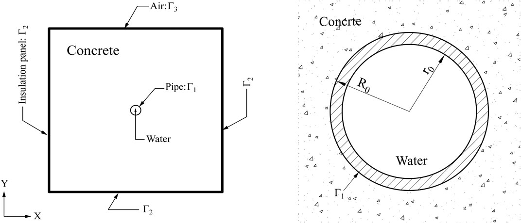
FIGURE 1. Calculation model for water-containing pipes.

In this equation $T$ is the unknown temperature; $\tau$ is the time; $\alpha$ is the concrete thermal diffusivity coefficient; $\theta$ is the adiabatic temperature rise.

The water pipes discussed in this article are of non-metallic material. Basis on [4], the inner boundary of the non-metallic water pipe is in contact with water, so the temperature is equal to the water temperature $T_w$. The outside of the water pipe is in contact with the inner surface of the concrete, and the temperature is equal to the temperature $T_c$ of the inner surface of the concrete. Thus, the heat flux $q$ from concrete to water pipe can be expressed as

$q=-{\beta }^{\prime }\left(T_w-T_c\right)(2)$

${\beta }^{\prime }=\frac{{\lambda }_1}{R_0\ln \left(R_0/r_0\right)}\cong \frac{{\lambda }_1}{R_0-r_0}(3)$

Among them: ${\beta }^{\prime }$ is the equivalent heat transfer coefficient of water pipe and concrete, and $h=R_0-r_0$ is the thickness of water pipe. When $h\to 0$, at this time ${\beta }^{\prime }\to \infty$, the contact surface between the water pipe and the concrete is equivalent to the first type of boundary condition. ${\lambda }_1$ is thermal conductivity coefficient of non-metallic water pipes; $R_0$ is the outer diameter of the water pipe; $r_0$ is the inner diameter of the water pipe, and $T_w$ is the water temperature of a given function. The method for calculating the water temperature is referred to Zhu [31].

Then the initial conditions and boundary conditions of the concrete with cooling water pipe can be expressed as the following formula

$\{\begin{array}{ll}T\left(\mathbf{x},0\right)=T_0\hfill & \mathbf{x}\in \Omega \hfill \\ \frac{\partial T\left(\mathbf{x},\tau \right)}{\partial \mathbf{n}}=\frac{{\beta }^{\prime }}{\lambda }\left(T_w-T\left(\mathbf{x},\tau \right)\right)\hfill & \mathbf{x}\in {\Gamma }_1\hfill \\ \frac{\partial T\left(\mathbf{x},\tau \right)}{\partial \mathbf{n}}=0\hfill & \mathbf{x}\in {\Gamma }_2\hfill \\ \frac{\partial T\left(\mathbf{x},\tau \right)}{\partial \mathbf{n}}=\frac{\beta }{\lambda }\left(T_a-T\left(\mathbf{x},\tau \right)\right)\hfill & \mathbf{x}\in {\Gamma }_3\hfill \end{array}(4)$

In this formula the initial temperature of the concrete is expressed in $T_0$; and $T_a$ is the atmospheric temperature; $\lambda$ is the thermal conductivity coefficient of concrete; and $\beta$ is heat transfer coefficient of concrete to air. Furthermore, ${\Gamma }_2$ represents the concrete adiabatic boundary. ${\Gamma }_3$ represents the boundary between concrete and air, and ${\Gamma }_1$ represents the boundary between water pipe and concrete.

Integration Scheme

Since the RPIM cannot convert the integrals in the solution domain into the sum of the integrals of the discrete units, this paper uses the background grid integral method to integrate the problem domain. The background grid integration method is to divide the problem domain into n regular background grids, and then use Gaussian integration to calculate numerically in each background grid, and finally superimpose the background grid integrals. In this paper, we call each background grid a background unit.

The background grid is used to integrate the function, and the formula is as follow

${\displaystyle \underset{\Omega }{\int }F\left(\mathbf{x}\right)d\Omega }={\displaystyle \sum _{k=1}^{N_c}{\displaystyle \underset{{\Omega }_k}{\int }F\left(\mathbf{x}\right)d{\Omega }_k}},\mathbf{x}\in \Omega (5)$

where

${\displaystyle \underset{{\Omega }_k}{\int }F\left(\mathbf{x}\right)}d{\Omega }_k={\displaystyle \sum _{r=1}^{N_r}{\stackrel{⌢}{w}}_r}F\left({\mathbf{x}}_r\right)\left|{\mathbf{J}}_{rk}\right|,{\mathbf{x}}_r\in \Omega (6)$

In the above formula, $N_c$ is the number of background grids, and ${\Omega }_k$ is the unit field of the k^th background grid. $N_r$ is the number of Gaussian integration points in ${\Omega }_k$, ${\stackrel{⌢}{w}}_r$ is the rth Gauss weight coefficient, and $\left|{\mathbf{J}}_{rk}\right|$ is the Jacobian matrix of the k^th background grid at the integration points ${\mathbf{x}}_r$.

Water Pipe Cooling Scheme

This paper uses the method [4] proposed to deal with the cooling effect of water pipes. The idea is to use the contact surface between concrete and water pipe as the boundary condition for heat dissipation and include the heat dissipation surface into the governing Eq. 1. The heat dissipation coefficient of the contact surface is estimated according to the thickness of the water pipe and the thermal conductivity. The solution of the three-dimensional transient temperature field of concrete with cooling water pipes is equivalent to the extreme value of the following functional

$\begin{array}{c}\prod ={\displaystyle \underset{V^e}{\iiint }\{\frac{\alpha }{2}\left[{\left(\frac{\partial T}{\partial x}\right)}^2+{\left(\frac{\partial T}{\partial y}\right)}^2+{\left(\frac{\partial T}{\partial z}\right)}^2\right]+\left(\frac{\partial T}{\partial \tau }-\frac{\partial \theta }{\partial \tau }\right)T\}}dv+{\displaystyle \underset{S^e}{\int }\overline{\beta }\left(\frac{1}{2}{T}^2-T_{a}T\right)ds}\\ +{\displaystyle \underset{S^{\prime }}{\int }{\beta }^{\prime }\left(\frac{1}{2}{T}^2-T_{w}T\right)ds}\end{array}(7)$

In the equation $V^e$, $S^e$, and $S^{\prime }$ are the domain of the background unit, the heat release surface of concrete and air, and the heat dissipation surface of the water pipe and concrete respectively.

The temperature of any point in the element can be obtained by linear interpolation of the element nodes.

$\mathbf{T}=T\left(\mathbf{x},\tau \right)={\displaystyle \sum _{i=1}^n{\varphi }_i{T}_i=\mathbf{\Phi }{\mathbf{T}}^e}(8)$

${\mathbf{T}}^{\prime }={\mathbf{T}}^{\prime }\left(\mathbf{x},\tau \right)={\displaystyle \sum _{i=1}^n{\varphi }_i\frac{\partial T_i}{\partial \tau }=\mathbf{\Phi }{{\mathbf{T}}^{\prime }}^e}(9)$

Among them: $\mathbf{T}$ is the overall node temperature; n is the number of field nodes in the support domain; ${\mathbf{T}}^e$ is the field node temperature in the support domain and $\dot{\mathbf{T}}$ is the derivative of temperature time.

Substituting Eqs 8, 9 into Eq. 7,

$\begin{array}{c}\Pi =\frac{1}{2}{\displaystyle \sum _e\left({\mathbf{T}}^e\right)}{\displaystyle {\int }_{V^e}\alpha }\left[\left(\frac{\partial {\mathbf{\Phi }}^T}{\partial x}\frac{\partial \mathbf{\Phi }}{\partial x}+\frac{\partial {\mathbf{\Phi }}^T}{\partial y}\frac{\partial \mathbf{\Phi }}{\partial y}+\frac{\partial {\mathbf{\Phi }}^T}{\partial z}\frac{\partial \mathbf{\Phi }}{\partial z}\right)\right]dv{\mathbf{T}}^e\\ +{\displaystyle \sum _e\left({\mathbf{T}}^e\right)}{\displaystyle {\int }_{V^e}\left({\mathbf{\Phi }}^T\mathbf{\Phi }\right)}dv{{\mathbf{T}}^{\prime }}^e-{{\displaystyle \sum _e\left({\mathbf{T}}^e\right)}}^T{\displaystyle {\int }_{V^e}\left({\mathbf{\Phi }}^T\frac{\partial \theta }{\partial \tau }\right)}dv\\ +\frac{1}{2}{{\displaystyle \sum _e\left({\mathbf{T}}^e\right)}}^T{\displaystyle {\int }_{S^e}\overline{\beta }\left({\mathbf{\Phi }}^T\mathbf{\Phi }\right)}ds{{\mathbf{T}}^{\prime }}^e-{{\displaystyle \sum _e\left({\mathbf{T}}^e\right)}}^T{\displaystyle {\int }_{S^e}\overline{\beta }\left({\mathbf{T}}_a{\mathbf{\Phi }}^T\right)}ds\\ +\frac{1}{2}{{\displaystyle \sum _e\left({\mathbf{T}}^e\right)}}^T{\displaystyle {\int }_{S^{\prime }}{\beta }^{\prime }\left({\mathbf{\Phi }}^T\mathbf{\Phi }\right)}ds{{\mathbf{T}}^{\prime }}^e-{{\displaystyle \sum _e\left({\mathbf{T}}^e\right)}}^T{\displaystyle {\int }_{S^{\prime }}{\beta }^{\prime }\left({\mathbf{T}}_w{\mathbf{\Phi }}^T\right)}ds\end{array}(10)$

Simplify the Eq. 10, we can obtain

$\Pi =\frac{1}{2}{\mathbf{T}}^T\left(\mathbf{H}+\mathbf{G}\right)\mathbf{T}+{\mathbf{T}}^T\mathbf{R}{\mathbf{T}}^{\prime }-{\mathbf{T}}^T\mathbf{F}(11)$

Where $\mathbf{H}+\mathbf{G}$ is global thermal transfer matrix, $\mathbf{F}$ is global temperature load matrix, and $\mathbf{R}$ is thermal capacity matrix.

According to the variational principle, the variation of Eq. 11 is $\delta \Pi =0$, and we can obtain:

$\left(\mathbf{H}+\mathbf{G}\right)\mathbf{T}+\mathbf{R}{\mathbf{T}}^{\prime }=\mathbf{F}(12)$

where

$\{\begin{array}{c}\mathbf{H}={\displaystyle \sum _e{\left[\mathbf{c}\right]}^T\left[\mathbf{h}\right]}\left[\mathbf{c}\right]\\ \mathbf{G}={\displaystyle \sum _e{\left[\mathbf{c}\right]}^T\left[\mathbf{g}\right]}\left[\mathbf{c}\right]\\ \mathbf{R}={\displaystyle \sum _e{\left[\mathbf{c}\right]}^T\left[\mathbf{r}\right]}\left[\mathbf{c}\right]\\ \mathbf{F}={\displaystyle \sum _e{\left[\mathbf{c}\right]}^T\left[\mathbf{f}\right]}\end{array}(13)$

$\left[\mathbf{c}\right]$ is the element selection matrix and

${\mathbf{T}}^e=\mathbf{c}\mathbf{T}(14)$

the element coefficient matrix is the following expression

$h_{ij}=\alpha {\displaystyle \underset{V^e}{\iiint }\left(\frac{\partial {\varphi }_i}{\partial x}\frac{\partial {\varphi }_j}{\partial x}+\frac{\partial {\varphi }_i}{\partial y}\frac{\partial {\varphi }_j}{\partial y}+\frac{\partial {\varphi }_i}{\partial z}\frac{\partial {\varphi }_j}{\partial z}\right)}dv(15)$

$g_{ij}=\overline{\beta }{\displaystyle \underset{S^e}{\iint }{\varphi }_i}{\varphi }_{j}ds+{\beta }^{\prime }{\displaystyle \underset{S^{\prime }}{\iint }{\varphi }_i{\varphi }_{j}ds}(16)$

$f_i={\displaystyle \underset{V^e}{\iiint }\frac{\partial \theta }{\partial \tau }}{\varphi }_{i}dv+\overline{\beta }{\displaystyle \underset{S^e}{\iint }{T}_a}{\varphi }_{i}ds+{\beta }^{\prime }{\displaystyle \underset{S^{\prime }}{\iint }{T}_w}{\varphi }_{i}ds(17)$

$r_{ij}={\displaystyle \underset{V^e}{\iiint }{\varphi }_i}{\varphi }_{j}dv(18)$

The last term in the above Eqs 16, 17 is the correction term for the cooling water pipe. In the formula $\overline{\beta }=\beta /c\rho$, $c$ is the specific heat capacity of concrete, and $\rho$ is the density of concrete.

During the construction of large-volume concrete, since the spacing of the cooling water pipes is much smaller than its length, and the heat of the concrete is mainly transmitted perpendicular to the water pipe, the integral of the water pipe contact surface can be converted into a one-dimensional integral along the direction of the water pipe. The expression of the correction term can be rewritten as

${\beta }^{\prime }{\displaystyle \underset{S^{\prime }}{\iint }{\varphi }_i{\varphi }_{j}ds}=2\pi R_0{\beta }^{\prime }{\displaystyle {\int }_{-1}^1{\varphi }_i}{\varphi }_j\frac{l}{2}d\xi (19)$

${\beta }^{\prime }{\displaystyle \underset{S^{\prime }}{\iint }{T}_w}{\varphi }_{i}ds=2\pi R_0{\beta }^{\prime }{\displaystyle {\int }_{-1}^1{T}_w{\varphi }_i\frac{l}{2}}d\xi (20)$

Where $l$ is the water pipe length in the background unit, and $T_w$ is the temperature of the water flow.

Time Discretization Scheme

The difference method is used to discretise the time term in Eq. 12, Firstly the time domain [0, t] is divided into $nt$ time steps. Then the time domain becomes $\left[{\tau }_0,{\tau }_1,\cdots ,{\tau }_{nt}\right]$ and the step size of each step is $\Delta \tau ={\tau }_{i+1}-{\tau }_i$. Assuming $\Delta \tau$ temperature changes linearly so

$T\left(\tau +s\Delta \tau \right)=s\left(T_{nt+1}-T_{nt}\right)-T_{nt}(21)$

$T^{\prime }\left(\tau +s\Delta \tau \right)=\frac{\left(T_{nt+1}-T_{nt}\right)}{\Delta \tau }(22)$

Taking $s=1$ as the backward difference method and asking the above Eqs 21, 22 into Eq. 12, we can obtain

$\left(\mathbf{K}+\frac{1}{\Delta \tau }\mathbf{R}\right){\mathbf{T}}_{nt+1}=\frac{1}{\Delta \tau }\mathbf{R}{\mathbf{T}}_{nt}+s{\mathbf{F}}_{nt+1}(23)$

By combining the initial and boundary conditions, the Eq. 23 can be used to solve the system of equations to obtain the field node temperature array at each time.

Radial Point Interpolation Method

The RPIM is formed by adding a set of PIM to the radial basis function (RBF), which overcomes the problem of matrix singularity caused by polynomial basis functions. The calculation principle of the RPIM is to take a set of field nodes in a small local domain for a calculation point and use a combination of an RBF and a polynomial to fit the value of the calculation point on the field node. RPIM interpolation can be expressed as:

$T\left(\mathbf{x}\right)={\displaystyle \sum _{i=1}^m{R}_i\left(\mathbf{x}\right)}{a}_i+{\displaystyle \sum _{j=1}^k{p}_j}\left(\mathbf{x}\right)b_j,\mathbf{x}\in \Omega (24)$

Where $T\left(\mathbf{x}\right)$ is the numerical solution of the calculation point. $R_i\left(\mathbf{x}\right)$ is the RBF. $m$ is the number of RBFs. $p_j\left(\mathbf{x}\right)$is a monomial of space coordinates, $k$ is the number of polynomial basis functions. $\mathbf{x}$ is the calculation point. $a_j$ and $b_j$ are unknown coefficients.

In order to obtain the unknown coefficients in the above Eq. 24, the RBF and the polynomial basis function are firstly determined. This paper uses the MQ-BRF method and first-order polynomial basis functions. The function expression is as follows:

The expression of the MQ-RBFs function is:

$R_i\left(\mathbf{x},{\mathbf{y}}_i\right)={\left({\left(\mathbf{x}-{\mathbf{y}}_i\right)}^2+{\left(w_{0}l\right)}^2\right)}^c,\mathbf{x},{\mathbf{y}}_i\in \Omega ,(25)$

Polynomial basis function expression of first degree:

$P_j^T\left(\mathbf{x}\right)=\left\{\begin{array}{cccc}1& x_j& y_j& z_j\end{array}\right\},x_j,y_j,z_j\in \Omega ,(26)$

$\mathbf{x}-{\mathbf{y}}_i$ is the distance between the calculation point $\mathbf{x}$ and the field node ${\mathbf{y}}_i$ in the local domain. Then ${\mathbf{r}}_i=\mathbf{x}-{\mathbf{y}}_i$ is used indicate the distance between them. $w_0$ and $c$ are shape parameters of MQ-RBF. This paper obtains these parameters c by trying a series of data. $l$ is the average distance of field nodes in the local domain. In order to obtain the unknown coefficients $a_i$ and $b_j$, a local domain needs to be formed at the calculation point $\mathbf{x}$, and RPIM uses the field nodes in the local domain to form $n$ linear equations.

Then Eq. 24 can be expressed in a matrix as

${\mathbf{T}}_s=\mathbf{R}\mathbf{a}+{\mathbf{P}}_k\mathbf{b}(27)$

the function value ${\mathbf{T}}_s={\left\{T_1,T_2,\mathrm{...},T_n\right\}}^T$.

The moment matrix of RBFs is equal to R:

$\mathbf{R}={\left[\begin{array}{cccc}{R}_1\left(r_1\right)& R_2\left(r_1\right)& \cdots & R_n\left(r_1\right)\\ R_1\left(r_2\right)& R_2\left(r_2\right)& \cdots & R_n\left(r_2\right)\\ \cdots & \cdots & \cdots & \cdots \\ R_1\left(r_n\right)& R_2\left(r_n\right)& \cdots & R_n\left(r_n\right)\end{array}\right]}_{n\times n}(28)$

The polynomial moment matrix is:

${\mathbf{P}}_k^T={\left[\begin{array}{cccc}1& 1& \cdots & 1\\ x_1& x_2& \cdots & x_n\\ y_1& y_2& \cdots & y_n\\ z_1& z_2& \cdots & z_n\\ ⋮& ⋮& \ddots & ⋮\\ p_k\left({\mathbf{x}}_1\right)& p_k\left({\mathbf{x}}_2\right)& \cdots & p_k\left({\mathbf{x}}_n\right)\end{array}\right]}_{\left(k\times n\right)}(29)$

Eq. 27 is written in matrix form:

$\left\{\begin{array}{c}\mathbf{a}\\ \mathbf{b}\end{array}\right\}={\left[\begin{array}{ll}\mathbf{R}\hfill & {\mathbf{P}}_k^T\hfill \\ {\mathbf{P}}_k\hfill & 0\hfill \end{array}\right]}^{-1}{\mathbf{T}}_s={\mathbf{A}}_0^{-1}{\mathbf{T}}_s(30)$

At this time, the unknown coefficients $\mathbf{a}$ and $\mathbf{b}$ are obtained, and the unknown coefficients $\mathbf{a}$ and $\mathbf{b}$ are brought back to Eq. 27 to obtain:

$T\left(\mathbf{x}\right)=\left\{{\mathbf{R}}^T\left(\mathbf{x}\right)P^T\left(\mathbf{x}\right)\right\}{\mathbf{A}}_0^{-1}{\mathbf{T}}_s={\mathbf{\Phi }}^T\left(\mathbf{x}\right){\mathbf{T}}_s,x\in {\Omega }_s(31)$

Where ${\mathbf{\Phi }}^T\left(x\right)=\left\{{\varphi }_1,{\varphi }_2,\cdots ,{\varphi }_n\right\}$ is the shape function of RPIM. The derivative of the numerical solutions are as follows:

$\partial \mathbf{T}\left(x\right)={\displaystyle \sum _{i=1}^n{T}_i\partial \Phi \left({\mathbf{x}}_i\right)}{\mathbf{x}}_i,\mathbf{x}\in {\Omega }_s(32)$

Here $\partial$ is a differential operator.

This paper adopts two methods to improve the accuracy so that these make the numerical solution have better accuracy. Firstly, it uses adaptive shape parameters $w$ in each supported domain ${\Omega }_s$. The formula is as follows:

$w=\frac{w_0}{\min \left(\Vert x-x_i\Vert \right)},x_i,x\in {\Omega }_s(33)$

Where $w_0$ stands for the initial shape parameter. $\mathbf{x}$ is the calculation point in the support domain and ${\mathbf{x}}_i$ is the field node in the support domain. Additionally, for the matrix in Eq. 12, this paper uses Liu [30] method to reduce the condition number of the matrix, thereby improving the stability of the algorithm.

Numerical Experiments

In this section, four examples are used to experimentally examine RPIM in terms of accuracy, stability, and convergence. To analyse the error of the numerical solution, relative error (RE), and the relative root mean square error (RMSE) are selected as the error-index.

$RE\left(T\right)=\left|\frac{T\left(x_i\right)-\widehat{T}\left(x_i\right)}{\widehat{T}\left(x_i\right)}\right|(34)$

$RMSE\left(T\right)=\sqrt{\frac{1}{N_c}{\displaystyle \sum _{i=1}^{N_c}{\left(T\left(x_i\right)-\widehat{T}\left(x_i\right)\right)}^2}}/\sqrt{\frac{1}{N_c}{\displaystyle \sum _{i=1}^{N_c}{\widehat{T}}^2\left(x_i\right)}}(35)$

$T\left(x_i\right)$ is the analytic solution or the exact solution of the FEM at the calculation point $x_i$, and $\widehat{T}\left(x_i\right)$ is the numerical solution of the RPIM. $N_c$ is the total number of test points.

Example 1

We verify the effectiveness of the algorithm through a two-dimensional calculation example. It supposes that the thin plate is a square and the side length is 1.6 m. The concrete domain uses 1,089 field nodes with an interval of 0.05 m. The adiabatic temperature rise of concrete is $\theta \left(\tau \right)=15\text{.}32\times \left(1-{\text{e}}^{-0.4{\tau }^{0.66}}\right)$ and thermal conductivity coefficient is $\alpha =\text{0}\text{.}1m^2/d$. The outer diameter of the water pipe is $R_0=0.016m$. The thickness is $\text{h}=0.002m$. The thermal conductivity of the water pipe is $\lambda =1\text{.}66kJ/\left(m·h·°C\right)$. The initial temperature is $T_0=20°C$ and the initial water temperature is $T_w=20°C$. The time step is $\Delta \tau =0.02\text{day}$.

Figure 2 shows the distribution of concrete temperature fields at different times. It can be seen that the results of the proposed method are basically consistent with those of the FEM. When simulating example 1, the FEM used 4,176 elements. The relative error is shown in Figure 3 also verifies the event, and the maximum error is near the water pipe and remains at about 2.3%. Other changes with time, the algorithm also maintains good stability. Through this example, the algorithm can accurately and effectively simulate the transient heat conduction problem of concrete with a cooling pipe in the rectangular region.

FIGURE 2

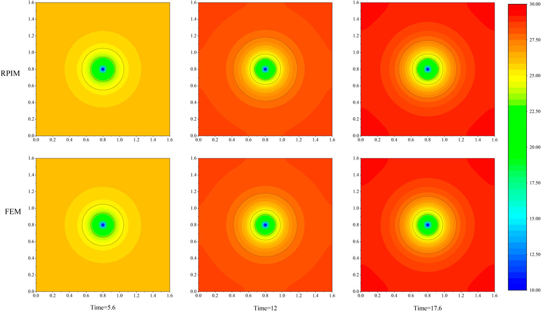
FIGURE 2. Comparison of temperature fields between numerical solution and fine solution at different times.

FIGURE 3

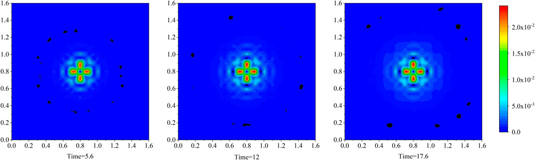
FIGURE 3. The relative error graph of numerical solution and fine solution.

Example 2

The example two considers the temperature field of cubic concrete under a single water pipe. Selecting the concrete block whose calculation domain is $\Omega =\{\left(x,y,x\right)|0<x,y,z<1.5m\}$. The concrete domain uses 1,375 field nodes, of which 1,331 (11 × 11 × 11) are evenly arranged with a spacing of 0.15 m. Adding four nodes around the water pipe is as shown in the picture of Figure 4A. The initial temperature of the concrete is 20°C, and the concrete surface is adiabatic. The material parameters of concrete and water pipes are shown in Table 1. The adiabatic temperature rise of concrete is $\theta \left(\tau \right)=21\text{.}66\times \left(1-{\text{e}}^{-0.49{\tau }^{0.56}}\right)$. The outer diameter of the water pipe is ${\text{R}}_0=0.016m$, the thickness is $\text{h}=0.002m$. The water temperature along the water pipe is obtained by linear interpolation of the inlet and outlet water temperature.

TABLE 1

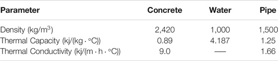
TABLE 1. Parameters of concrete and water pipe.

FIGURE 4

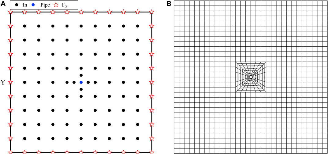
FIGURE 4. (A) RPIM field node and water pipe layout diagram. (B) FEM meshing diagram.

The flow velocity is $q_w=1.0m^3/h$ and the Initial water temperature is $T_w=5°\mathrm{C}$. Concrete continues to flow for 20 days. The time step is $\Delta \tau =0.1\text{day}$. The refined solution uses 11760 Element and is refined around the water pipe, as shown in the picture of Figure 4B.

In this case, selecting point 1(0.6,1.5,0.6), point 2(0.45,1.2,0.45), point 3(0.75,0.75,1.5), three points are as the test points. Figure 5A shows the numerical solution and the FEM fine solution of the test point over time. It can be concluded from the figure that the fine solution of the test point is basically consistent with the numerical solution. Figure 5B shows that the relative error between the fine solution and the numerical solution of the three test points is below 1E-2. Especially in the near water pipe point1 position, it still maintains better accuracy. Therefore, it is proved that the proposed water pipe embedding method is accurate and effective in combination with the RPIM method under the three-dimensional model.

FIGURE 5

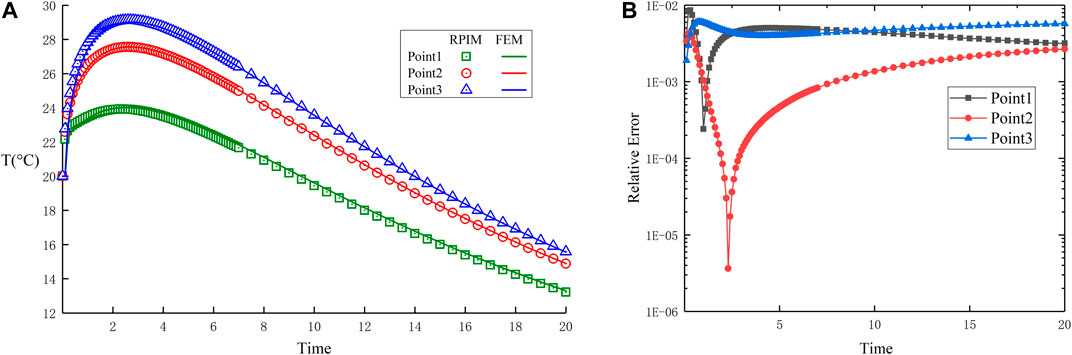
FIGURE 5. (A) Comparison of the numerical solutions obtained by FEM and RPIM temperature change over time at test points. (B) The RE of FEM and RPIM over time at the test point.

The Example two also verifies the convergence of the algorithm. Table 2 shows the RMSE values of the three test points at different time steps. It can be seen from the table that as the step size $\Delta \tau$ decreases, the RMSE also decreases. It shows that the algorithm is gradually converging. In addition, when the number of nodes in the field is the same, when the time step is less than $\Delta \tau =0.2\text{day}$, the RMSE values are basically equal, indicating that the numerical solution obtained by RPIM has converged when $\Delta \tau =0.2\text{day}$.

TABLE 2

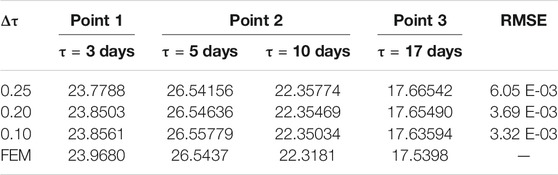
TABLE 2. Comparison of numerical and refine solutions under different time increment conditions, for Example two.

This calculation example takes into account the water temperature change along the route and the heat conduction of concrete containing the cooling water pipe is discussed under the third boundary condition. The result shows that the algorithm has good properties in precision, stability, and convergence under the above conditions.

Example 3

This example studies the influence of flow velocity, water temperature, and pipe diameter on the concrete temperature field based on example 2. Except for water flow velocity, water temperature, and pipe inner diameter, other parameters are the same as those in calculation example 2. The water flow time is 20 days.

Tables 3–5 respectively list the flow velocity, water temperature, and the change of the parameters of the pipe inner diameter.

TABLE 3

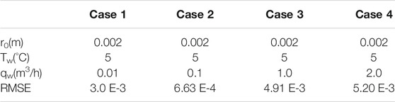
TABLE 3. RMSE value at different flow velocity, for Example three.

TABLE 4

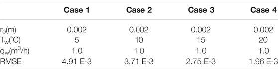
TABLE 4. RMSE value at different water temperature, for Example three.

TABLE 5

TABLE 5. RMSE value at different pipe inner diameter, for Example three.

In this example, when discussing the influence of parameter changes on the temperature field, the highest temperature of concrete is selected for discussion. Table 3 discusses the influence of cooling water pipe flow velocities changes on the temperature field and selects four different flow velocities. Figure 6A shows that the temperature of the concrete is greatly reduced after the cooling water pipe is added, and the maximum temperature is only about 30°C while the temperature field without adding water pipes still keeps rising after the 20^th day and is above 40°C. Under the latter three conditions, the temperature curve did not change much, and the maximum temperature difference was only 0.3°C, which indicates that when the flow velocities reached a certain level, increasing the flow velocities did not significantly improve the cooling effect.

FIGURE 6

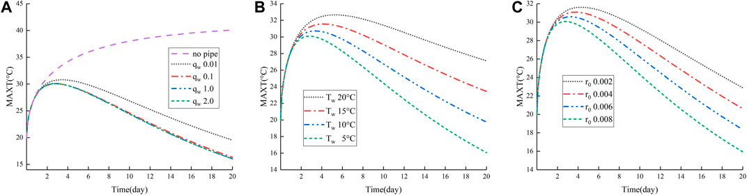
FIGURE 6. (A) The maximum temperature of concrete at different flow rates. (B) The maximum temperature of concrete under different water temperatures. (C) The maximum temperature of concrete under different pipe inner diameters.

Table 4 shows the changes in water temperature parameters. Figure 6B shows the maximum temperature value after the water temperature changes. The maximum concrete temperature is 30.1°C under 5°C water temperature. And the maximum concrete temperature is 32.7°C under 20°C water temperature. It is not particularly obvious the difference in temperature between the highest temperatures from 5°C to 20°C. But after the 4th day, the water temperature becomes lower and then the faster temperature of the concrete will drop. The temperature difference of the highest temperature on the 20^th day is 11.1°C. It shows that the water temperature has a great influence on the change of concrete temperature. But, when the water temperature is too low, a large temperature gradient will be generated near the water pipe, which will occur a large local tensile stress and cause damage the structure. Therefore, the cooling water temperature should not be too low during actual construction.

Table 5 shows the Change in r₀ of the water pipe. Figure 6C shows that changing the r₀ of the water pipe still has a greater impact on the temperature of the concrete. When r₀ gradually becomes smaller, the heat dissipation capacity of the water pipe becomes worse. The reason is that when the water pipe r₀ becomes smaller, its heat transfer coefficient β′ becomes smaller, and the amount of heat transferred per unit condition decreases, resulting in poor heat dissipation effect. The effective contact area of other water pipes with water and the decrease in the flow rate per unit time of the water pipe are also factors that cause the deterioration of the heat dissipation capacity of the water pipe. Therefore, if the r₀ of the water pipe increases, then the temperature of the concrete will drop accordingly.

The RMSE values in Tables 3–5 have always been maintained under 1E-2, which verified that this method has good accuracy, stability, and robustness for the heat transfer of the three-dimensional concrete model below the third kind of boundary conditions under the condition of water flow.

Example 4

Based on the two calculation examples 2 and 3, we have added multiple water pipes to the concrete model in example four and have increased the boundary conditions of the heat exchange between the concrete surface and the air. The size of the concrete model is $\Omega =\left\{\left(x,y,z\right)|0<x<3m,0<y<2m,0<z<1m\right\}$. Arranged three water pipes in the direction parallel to the Y axis, it is as shown in Figure 7A. In this example, the model has a total of 2,046 (31 × 11 × 6) field nodes, of which 18 (6 × 3) water pipes are arranged. Figure 7B shows the layout of field nodes and boundary conditions. It is worth noting that the material parameters of concrete and water pipes are the same as those in Example 2, such as the water flow velocity and the initial water temperature. The boundary temperature of ${\Gamma }_3$ is $T_a=30°\text{C}$. The initial temperature of concrete and water pipe is 20°C, and the other boundaries are insulated. At the same time, the water supply time is also time = 20 days.

FIGURE 7

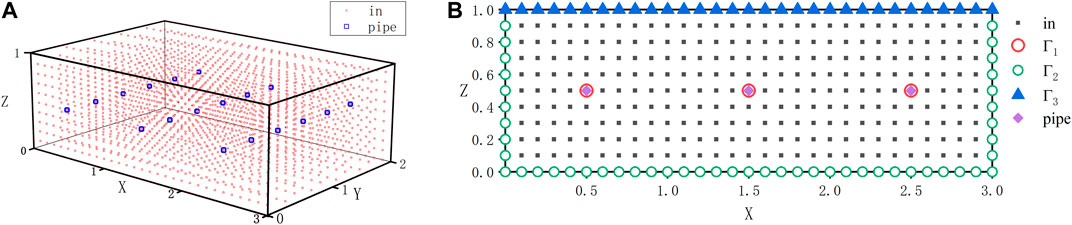
FIGURE 7. (A) Layout patterns of field nodes and water pipes. (B) Boundary condition layout pattern.

For the three-dimensional model, we choose point 1 (0.0, 2.0, 1.0), point 2 (0.6, 2.0, 0.6), point 3 (1.8, 0.8, 0.5) three points and the FEM fine solution for discussion. (The FEM calculation includes 17520 elements). Figure 8A shows the numerical solution and fine solution of RPIM under the time-varying three test points. Consequently, the result is that the numerical solution of the algorithm can still maintain high accuracy under the condition of multi-water pipe. It can also be concluded from the relative error graph in Figure 8B that the error between the test point and the fine solution is below 1E-2, especially at point 2 near the water pipe. In actual engineering calculations, the accuracy of the algorithm is sufficient.

FIGURE 8

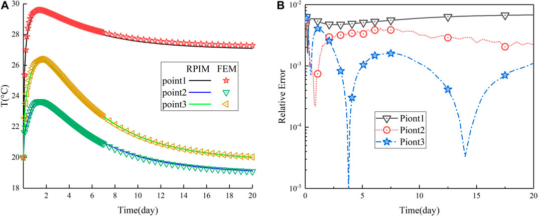
FIGURE 8. (A) With time changed, numerical solution of FEM and RPIM at test points. (B) The RE of FEM and RPIM at the test point changes over time.

Table 6 shows the comparison between the numerical solution and the fine solution of the test points under different total numbers of field nodes. And Table 6 shows that as the total number of field nodes increases, the RMSE gradually decreases, which indicates that the convergence of the algorithm is also better under multiple water pipes. Furthermore, in terms of calculation time, the more the number of field nodes, the more time it takes. But compared with the FEM algorithm, it only takes 220 s to reach an accuracy of 1E-3.

TABLE 6

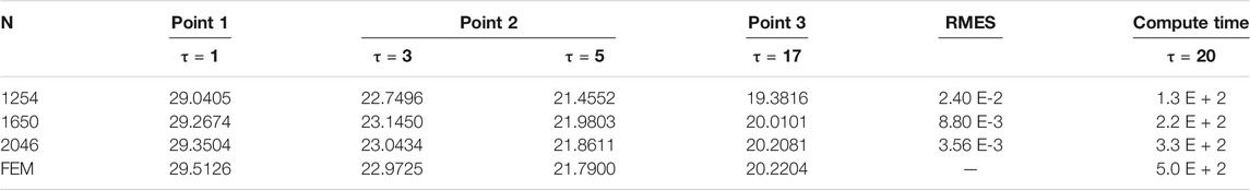
TABLE 6. RMSE of numerical solution and refine solution varies with time under different field nodes, for Example four.

This example also compares the maximum temperature difference $\Delta T$ between the inside and the surface of the concrete. The Maximum temperature difference including pipes is ΔT = 19.4°C. According to the engineering experience, the safety value of the temperature difference between the inside and surface of the concrete should be less than 25°C, so the water pipe layout in this paper is in line with the actual project. In conclusion, for the temperature field problem of concrete with cooling water pipes, the method proposed in this paper has high accuracy for temperature simulation, and it is valuable to apply it to actual engineering.

Conclusion

This paper uses the global weak-form radial basis function method and the method of ‘embedded water pipe’ to simulate the temperature field of concrete containing cooling water pipes. By incorporating the contact surface between the water pipe and the concrete as the heat dissipation surface into the governing equation, this reduces the modelling of water pipes. Using a Two-Side Equilibration Method and adaptive shape parameter method to further improve the accuracy and stability of the algorithm, and the discussion of four examples, it can be concluded that the algorithm can provide accurate prediction results. In conclusion, the method proposed in this paper has advantages in simulating the temperature field of hydration heat of concrete containing cooling water pipes.

The following conclusions can be drawn:

1) This method not only reduces the calculation cost, but also maintains the calculation accuracy.

2) The method is simple and convenient applying to actual projects, which still has good accuracy.

3) The method has good performance in stability, accuracy, and convergence.

Data Availability Statement

The raw data supporting the conclusions of this article will be made available by the authors, without undue reservation.

Author Contributions

FZ put forward the idea and completed all the paper of writing. GC give some suggestion to this paper. FZ check the errors in the program. QL sorted out the data.

Conflict of Interest

The authors declare that the research was conducted in the absence of any commercial or financial relationships that could be construed as a potential conflict of interest.

Publisher’s Note

All claims expressed in this article are solely those of the authors and do not necessarily represent those of their affiliated organizations, or those of the publisher, the editors and the reviewers. Any product that may be evaluated in this article, or claim that may be made by its manufacturer, is not guaranteed or endorsed by the publisher.

References

1. Bofang Z. Equivalent Equation of Heat Conduction in Mass concrete Considering the Effect of Pipe Cooling. J Hydraul Eng (1991) 3:28–34.

Google Scholar

2. Kim JK, Kim KH, Yang JK. Thermal Analysis of Hydration Heat in concrete Structures with Pipe-Cooling System. Comput Struct (2001) 79:163–71. doi:10.1016/S0045-7949(00)00128-0

CrossRef Full Text | Google Scholar

3. Zuo Z, Hu Y, Li Q, Liu G. An Extended Finite Element Method for Pipe-Embedded Plane thermal Analysis. Finite Elem Anal Des (2015) 102-103:52–64. doi:10.1016/j.finel.2015.05.002

CrossRef Full Text | Google Scholar

4. Chen G, Xu W, Yang Y, Li K. Computation Method for Temperature Field of Mass concrete Containing Cooling Water Pipes. Chin J Comput Phys (2012) 29:411–6. doi:10.19596/j.cnki.1001-246x.2012.03.015

CrossRef Full Text | Google Scholar

5. Belytschko T, Krongauz Y, Organ D, Fleming M, Krysl P. Meshless Methods: an Overview and Recent Developments. Comput Methods Appl Mech Eng (1996) 139:3–47. doi:10.1016/S0045-7825(96)01078-X

CrossRef Full Text | Google Scholar

6. Nguyen VP, Rabczuk T, Bordas S, Duflot M. Meshless Methods: A Review and Computer Implementation Aspects. Math Comput Simul (2008) 79:763–813. doi:10.1016/j.matcom.2008.01.003

CrossRef Full Text | Google Scholar

7. Belytschko T, Lu YY, Gu L. Element-free Galerkin Methods. Int J Numer Meth Engng (1994) 37:229–56. doi:10.1002/nme.1620370205

CrossRef Full Text | Google Scholar

8. Cheng H, Peng MJ, Cheng YM. A Hybrid Improved Complex Variable Element-free Galerkin Method for Three-Dimensional Potential Problems. Eng Anal Boundary Elem (2017) 84:52–62. doi:10.1016/j.enganabound.2017.08.001

CrossRef Full Text | Google Scholar

9. Cheng YM, Bai FN, Peng MJ. A Novel Interpolating Element-free Galerkin (IEFG) Method for Two-Dimensional Elastoplasticity. Appl Math Model (2014) 38:5187–97. doi:10.1016/j.apm.2014.04.008

CrossRef Full Text | Google Scholar

10. Atluri S, Liu H, Han Z. Meshless Local Petrov-Galerkin (MLPG) Mixed Finite Difference Method for Solid Mechanics. Comput Model Eng Sci (2006) 15:1. doi:10.3970/cmes.2006.015.001

CrossRef Full Text | Google Scholar

11. Atluri SN, Zhu T. A New Meshless Local Petrov-Galerkin (MLPG) Approach in Computational Mechanics. Comput Mech (1998) 22:117–27. doi:10.1007/s004660050346

CrossRef Full Text | Google Scholar

12. Honarbakhsh B. Numerical Solution of EFIE Using MLPG Methods. Eng Anal Boundary Elem (2017) 80:199–217. doi:10.1016/j.enganabound.2017.02.017

CrossRef Full Text | Google Scholar

13. Liu GR, Gu YT. Meshless Local Petrov-Galerkin (MLPG) Method in Combination with Finite Element and Boundary Element Approaches. Comput Mech (2000) 26:536–46. doi:10.1007/s004660000203

CrossRef Full Text | Google Scholar

14. Bui HH, Sako K, Fukagawa R. Numerical Simulation of Soil-Water Interaction Using Smoothed Particle Hydrodynamics (SPH) Method. J Terramechanics (2007) 44:339–46. doi:10.1016/j.jterra.2007.10.003

CrossRef Full Text | Google Scholar

15. Chen JK, Beraun JE, Jih CJ. An Improvement for Tensile Instability in Smoothed Particle Hydrodynamics. Comput Mech (1999) 23:279–87. doi:10.1007/s004660050409

CrossRef Full Text | Google Scholar

16. Colagrossi A, Landrini M. Numerical Simulation of Interfacial Flows by Smoothed Particle Hydrodynamics. J Comput Phys (2003) 191:448–75. doi:10.1016/S0021-9991(03)00324-3

CrossRef Full Text | Google Scholar

17. Hashemi MR, Fatehi R, Manzari MT. A Modified SPH Method for Simulating Motion of Rigid Bodies in Newtonian Fluid Flows. Int J Non Linear Mech (2012) 47:626–38. doi:10.1016/j.ijnonlinmec.2011.10.007

CrossRef Full Text | Google Scholar

18. Hashemi MR, Fatehi R, Manzari MT. SPH Simulation of Interacting Solid Bodies Suspended in a Shear Flow of an Oldroyd-B Fluid. J Non-Newtonian Fluid Mech (2011) 166:1239–52. doi:10.1016/j.jnnfm.2011.08.002

CrossRef Full Text | Google Scholar

19. Liu MB, Liu GR. Smoothed Particle Hydrodynamics (SPH): an Overview and Recent Developments. Arch Computat Methods Eng (2010) 17:25–76. doi:10.1007/s11831-010-9040-7

CrossRef Full Text | Google Scholar

20. Liew KM, Ng TY, Wu YC. Meshfree Method for Large Deformation Analysis-A Reproducing Kernel Particle Approach. Eng Struct (2002) 24:543–51. doi:10.1016/S0141-0296(01)00120-1

CrossRef Full Text | Google Scholar

21. Liu WK, Jun S, Zhang YF. Reproducing Kernel Particle Methods. Int J Numer Meth Fluids (1995) 20:1081–106. doi:10.1002/fld.1650200824

CrossRef Full Text | Google Scholar

22. Weng YJ, Zhang Z, Cheng YM. The Complex Variable Reproducing Kernel Particle Method for Two-Dimensional Inverse Heat Conduction Problems. Eng Anal Boundary Elem (2014) 44:36–44. doi:10.1016/j.enganabound.2014.04.008

CrossRef Full Text | Google Scholar

23. Liu GR, Gu YT. A point Interpolation Method for Two-Dimensional Solids. Int J Numer Meth Engng (2001) 50:937–51. doi:10.1002/1097-0207(20010210)50

CrossRef Full Text | Google Scholar

24. Askour O, Mesmoudi S, Braikat B. On the Use of Radial Point Interpolation Method (RPIM) in a High Order Continuation for the Resolution of the Geometrically Nonlinear Elasticity Problems. Eng Anal Boundary Elem (2020) 110:69–79. doi:10.1016/j.enganabound.2019.09.015

CrossRef Full Text | Google Scholar

25. Do VNV, Lee C-H. Bending Analyses of FG-CNTRC Plates Using the Modified Mesh-free Radial point Interpolation Method Based on the Higher-Order Shear Deformation Theory. Compos Struct (2017) 168:485–97. doi:10.1016/j.compstruct.2017.02.055

CrossRef Full Text | Google Scholar

26. Do VNV, Tran MT, Lee C-H. Nonlinear thermal Buckling Analyses of Functionally Graded Plates by a Mesh-free Radial point Interpolation Method. Eng Anal Boundary Elem (2018) 87:153–64. doi:10.1016/j.enganabound.2017.12.001

CrossRef Full Text | Google Scholar

27. Wang JG, Liu GR. A point Interpolation Meshless Method Based on Radial Basis Functions. Int J Numer Meth Engng (2002) 54:1623–48. doi:10.1002/nme.489

CrossRef Full Text | Google Scholar

28. Shivanian E. Analysis of Meshless Local and Spectral Meshless Radial point Interpolation (MLRPI and SMRPI) on 3-D Nonlinear Wave Equations. Ocean Eng (2014) 89:173–88. doi:10.1016/j.oceaneng.2014.08.007

CrossRef Full Text | Google Scholar

29. Hong Y, Lin J, Chen W. Simulation of thermal Field in Mass concrete Structures with Cooling Pipes by the Localized Radial Basis Function Collocation Method. Int J Heat Mass Transfer (2019) 129:449–59. doi:10.1016/j.ijheatmasstransfer.2018.09.037

CrossRef Full Text | Google Scholar

30. Liu C. A Two-Side Equilibration Method to Reduce the Condition Number of an Ill-Posed Linear System. Compr Model Eng Sci (2013) 91:17. doi:10.3970/cmes.2013.091.017

CrossRef Full Text | Google Scholar

31. Bofang Z Compound Methods for Computing the Effect of Pipe Cooling in Concrete Dams.Water Res Environ Eng (2003) 11:47–50. doi:10.13928/j.cnki.wrahe.2003.11.016

Google Scholar