Lattice Boltzmann Simulation of Multicomponent Porous Media Flows With Chemical Reaction

Flows with chemical reactions in porous media are fundamental phenomena encountered in many natural, industrial, and scientific areas. For such flows, most existing studies use continuum assumptions and focus on volume-averaged properties on macroscopic scales. Considering the complex porous structures and fluid–solid interactions in realistic situations, this study develops a sophisticated lattice Boltzmann (LB) model for simulating reactive flows in porous media on the pore scale. In the present model, separate LB equations are built for multicomponent flows and chemical species evolutions, source terms are derived for heat and mass transfer, boundary schemes are formulated for surface reaction, and correction terms are introduced for temperature-dependent density. Thus, the present LB model offers a capability to capture pore-scale information of compressible/incompressible fluid motions, homogeneous reaction between miscible fluids, and heterogeneous reaction at the fluid–solid interface in porous media. Different scenarios of density fingering with homogeneous reaction are investigated, with effects of viscosity contrast being clarified. Furthermore, by introducing thermal flows, the solid coke combustion is modeled in porous media. During coke combustion, fluid viscosity is affected by heat and mass transfer, which results in unstable combustion fronts.

1 Introduction

Flows of miscible fluids in porous media are frequently encountered in natural and industrial processes, like underground water movement [1], geologic carbon sequestration [2], enhanced oil recovery [3], and blood transport [4]. Dynamics of such flows are complex due to the unsteady flow, heat and mass transfer, and porous structure involved [5]. This situation becomes more complicated when chemical reactions are introduced.

In a porous medium, two fluids containing chemical solutes are put into contact along an interface. Chemical solutes are transported through the interface to react and thereby modify fluid properties, like density and viscosity. Meanwhile, if density or viscosity gradients exist across the interface, density or viscosity fingering may develop during the fluid transport [6]. Thus, interplay between interface instability and chemical reaction ensues. Such phenomena have been studied, for example, in systems containing ester-alkaline or CO₂-alkaline miscible solutions. Experiments were carried out to show that changes in chemical solutes modified the reaction type and intensity, leading to either enhanced or suppressed density fingering [7–10]. In parallel, theoretical analyses were conducted to predict viscous or density fingering scenarios with the reaction A + B → C [11–13]. In a porous medium with a partially miscible interface between the two fluids, Loodts et al. [11] suggested that different density contributions and diffusion rates of the three chemical species (A, B, and C) could introduce eight types of density profiles. Trevelyan et al. [12] theoretically showed that such a problem with a miscible interface could yield up to sixty-two types of density profiles. Each profile potentially represented a unique type of density fingering. As for viscous fingering with the reaction A + B → C, a linear stability analysis predicted and classified various fingering scenarios in a parameter plane spanned by viscosity ratios [13]. Under the guidance of theoretical predictions, efforts have been devoted to numerical simulations of interface instabilities with chemical reactions in porous media. For instance, Loodts et al. [14] numerically showed that the reaction A + B → C could accelerate, inhibit, or introduce the development of density fingering. They further demonstrated that different species diffusion rates could introduce four fingering types [15]. Numerical simulations were also performed to model viscous fingering dynamics with the reaction A + B → C [16]. Results suggested that the reaction could introduce a non-monotonic viscosity profile and thereby trigger the development of fingering. These simulations provided spatial and temporal properties of interface instabilities with chemical reactions, thus enriching experimental and theoretical findings.

The above studies focused on porous media flows with a homogeneous reaction between miscible fluids. On the other hand, a heterogeneous reaction can take place between fluid and solid phases. Explicitly, such a type of reaction consumes chemical solutes from the fluid phase and solid matrices to yield dissolved (dissolution reaction) or solid (precipitation reaction) products, which subsequently modifies medium structures and flow motions [17]. Until now, porous media flows with heterogeneous reactions have been extensively investigated. For example, acid dissolution experiments showed that the dissolution reaction increased medium porosity behind the moving fluid interface and thereby triggered fingering phenomena (or infiltration instability) [6, 18]. Fredd and Fogler were among the first to experimentally identify different fingering channels under various flow and dissolution rates [19]. The fingering phenomena induced by the dissolution reaction were observed to be destabilized by medium heterogeneity and brine pH [20]. In parallel, experiments on porous media flows with precipitation reactions showed that the reaction could generate a locally adverse mobility gradient to cause the onset of fingering [21]. The interplay between viscous fingering and precipitation reaction was experimentally studied, with the influencing factors and fingering shapes being clarified [22]. In the meantime, numerical simulations of porous media flows with heterogeneous reactions were conducted. For instance, fingering dynamics induced by dissolution reactions were tracked and compared on different simulation length scales [23]. Continuum models were built to describe fingering properties and classify different fingering regimes under the effects of chemical dissolution [24, 25]. In the presence of precipitation reactions, viscous fingering was modeled and found to be intensified [26, 27]. In some applications, like in situ combustion for heavy oil recovery, the combustion between hot air and solid fuels, as a typical form of heterogeneous reaction, releases heat to change fluid properties [28]. Thus, thermal flows were included in numerical studies on porous media flows with heterogeneous reaction. Field-scale modeling of solid coke combustion suggested the important role of heat conduction in stabilizing the combustion front [29] and identified key factors influencing the coke combustion rate and the front sweep efficiency [30, 31].

Overall, for porous media flows with chemical reactions, existing works focus on using empirical correlations and volume-averaged techniques to determine effective flow and reaction properties on microscopic scales. However, pore-scale information is necessary to provide further understanding of the microscopic phenomena involved [32]. In the past 3 decades, the lattice Boltzmann (LB) method has been developed and has become a powerful solver for porous media flows on the pore scale. This is attributed to its attractive advantages, like its general kinetic foundation, high parallelism, and ability to handle multiphysics and complex boundaries [33, 34]. Recently, LB models have been proposed to simulate flows of reactive fluids in porous media, like methane hydrate dissolution [35], solid coke combustion [32], and reactive mixing with viscous fingering [36]. Although these works showed the superior ability of the LB method in modeling porous media flows, some limitations should be noted. For example, changes in fluid density or viscosity with temperature are usually not accounted for, models for multicomponent reactions (like A + B → C) are underdeveloped, and iterative boundary schemes for conjugate heat transfer are complex and time-consuming. We have developed a series of LB models to overcome these shortcomings separately [37–40]. Nevertheless, a uniform LB model is still needed. This work thus proposes an LB model to simulate pore-scale reactive flows in porous media, with homogeneous and heterogeneous reactions and compressible and incompressible fluid densities being considered.

2 Mathematical Model

In a porous medium with porosity ϕ, a fluid 2 of solute B initially fills the pore spaces between solid matrices. Another fluid 1 of solute A is put into contact with fluid 2 along an interface. The two fluids are assumed to be miscible and have their own species concentration, viscosity, temperature, and density, which are noted by subscripts 1 and 2, respectively. As an example, a schematic of the fluid distribution with a vertical interface is shown in Figure 1. Once fluid transport starts, the two solutes A and B come into contact and react in the mixing zone as follows:

$A+B\to C+Q.(1)$

FIGURE 1

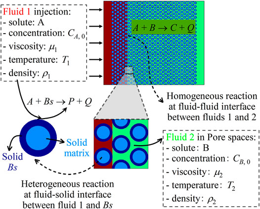
FIGURE 1. Schematic of the flow configuration with chemical reactions in porous media.

The reaction product C is in the dissolved form, Q is the reaction heat, and the reaction rate of this homogeneous reaction is R_o. Meanwhile, the nonreactive solid matrices can be coated with a reactive solid Bs to react with A as follows:

$A+Bs\to P+Q.(2)$

The product P is in either the dissolved or the solid form, representing the dissolution or the precipitation reaction, respectively. It should be noted that fluid 2 does not contain solute A, and thus, this heterogeneous reaction only takes place at the interface I between fluid 1 and solid Bs. With this heterogeneous reaction, solid Bs is dissolved gradually, and the update of the porous structure is tracked as follows [41]:

${\partial }_t{V}_B=-S_B{V}_{Bm}{R}_e,(3)$

where V_B and V_Bm are the volume and the molar volume of solid Bs, respectively, and S_B is the reactive surface area. The reaction rate of this heterogeneous reaction is noted as R_e.

The above homogeneous and heterogeneous reactions usually cause variations in fluid properties (like concentration, temperature, density, and viscosity) and medium structures, which subsequently alter flow motions in porous media. We seek to study the fluid transport properties of such a system, focusing on effects of chemical reactions. Evolutions of fluid flow and species concentrations in pore spaces are described by the following conservation equations:

${\partial }_t{\rho }_l+\nabla \cdot \left({\rho }_l\mathit{u}\right)=0,(4)$

${\partial }_t\left({\rho }_l\mathit{u}\right)+\nabla \cdot \left({\rho }_l\mathit{u}\mathit{u}\right)=-\nabla p+\nabla \cdot \left(\nu {\rho }_l\nabla \mathit{u}\right)+\mathit{F},(5)$

${\partial }_t\left({\rho }_l{Y}_r\right)+\nabla \cdot \left({\rho }_l{Y}_r\mathit{u}\right)=\nabla \cdot \left(D_r{\rho }_l\nabla Y_r\right)+S_r.(6)$

where $\mathit{u}=\left(u,v\right)$, ρ_l, p, and ν are the fluid velocity, density, pressure, and kinematic viscosity, respectively. t is the time, and F is the body force. Y_r is the mass fraction of species r (r = A, B, C, P), and it is related to species concentration as C_r = ρ_lY_r/M_r, with M_r being the species molecular weight. D_r and S_r are the diffusion coefficient and the homogeneous reaction source term of species r (Eq. 1), respectively. Furthermore, chemical reactions in Eqs 1, 2 usually release heat to change the local temperature, which in turn modifies the reaction rate and fluid properties. For such a consideration, heat transfer in both the fluid and solid phases is built as follows:

${\partial }_t\left(\rho c_{p}T\right)+\nabla \cdot \left(\rho c_{p}T\mathit{u}\right)=\nabla \cdot \left(\alpha \rho c_p\nabla T\right)+Q.(7)$

Here T, c_p, α, and ρ are the local temperature, specific heat at constant pressure, thermal diffusivity, and density, respectively. In addition, at the interface I between solute A and solid Bs, the heterogeneous reaction Eq. 2 is described as follows [32, 41]:

$\begin{array}{ll}\hfill \text{No}-\text{slip\hspace{0.17em}velocity:}& {\mathit{u}}^I=\left(0,0\right),\hfill \end{array}(8)$

$\begin{array}{ll}\hfill \text{Species\hspace{0.17em}conservation:}& \mathit{n}\cdot \frac{D_r{\rho }_l}{M_r}\nabla Y_r^I=a_r{R}_e,\hfill \end{array}(9)$

$\begin{array}{ll}\hfill \text{Conjugate\hspace{0.17em}heat\hspace{0.17em}transfer:}& \left\{\begin{array}{c}{T}^{I,+}=T^{I,-},\hfill \\ \mathit{n}\cdot {\left(k\nabla T+\rho c_p\mathit{u}T\right)}^{I,+}=\mathit{n}\cdot {\left(k\nabla T+\rho c_p\mathit{u}T\right)}^{I,-}+q,\hfill \end{array}\right.\hfill \end{array}(10)$

where n is the interface normal pointing to the fluid phase, + and − denote parameters on either side of I, k = αρc_p is the local thermal conductivity, q is the reaction heat flux, and a_r is the stoichiometric coefficient of species r.

By introducing the characteristic length L, velocity U, temperature T_ch, concentration C_ch, and density ρ_ch, dimensionless parameters marked by asterisks are derived as follows:

$\begin{array}{c}{x}^{*}=\frac{x}{L},y^{*}=\frac{y}{L},t^{*}=\frac{t}{L/U},{\mathit{u}}^{*}=\frac{\mathit{u}}{U},T^{*}=\frac{T}{T_{ch}},C_r^{*}=\frac{C_r}{C_{ch}},\\ {\mathit{F}}^{*}=\frac{\mathit{F}}{{\rho }_{ch}{U}^2/L},\text{Re}=\frac{LU}{{\nu }_2},{\text{Pe}}_r=\frac{LU}{D_r},\mathrm{Pr}=\frac{{\nu }_2}{{\alpha }_l},\text{Sc}=\frac{{\nu }_2}{D_r},\end{array}(11)$

Key characteristic numbers are as follows: the Reynolds number Re, the Peclet number Pe, the Prandtl number Pr, and the Schmidt number Sc.

It is emphasized that the above equations consider homogeneous and heterogeneous reactions via the source term S_r and boundary conditions Eqs. 8–10, respectively. Evolutions of chemical species are described using Eq. 6 separately, thus allowing for homogeneous reactions between multiple solutes. Furthermore, both compressible and incompressible fluid flows can be taken into account, by setting the fluid density as a constant and a variable, respectively. On one hand, for compressible flows, the inclusion of heat transfer brings in the temperature-dependent fluid density. On the other hand, for incompressible flows, the thermophysical properties in Eq. 7 are fixed as constants in the fluid phase ϑ_l = ϑ₀ (ϑ = c_p, α, ρ), which can be different from those in the solid phase, namely, ϑ_s ≠ ϑ_l.

3 Lattice Boltzmann Model

An LB model is now developed to solve the above governing equations for porous media flows with chemical reactions. For pore-scale simulations, the multiple-relaxation-time (MRT) scheme was shown to be able to correctly capture the no-slip velocity condition at the fluid–solid boundary and avoid the unphysical dependence of permeability on viscosity [42–44]. The MRT collision operator is thus employed in our model development. Considering that this work focuses on reactive fluid flows in two-dimensional (2D) porous media, the most popular two-dimensional nine-velocity (D2Q9) scheme is applied, with the discrete velocities e_i and weight coefficients w_i being as follows [34]:

$\left\{\begin{array}{cc}{\mathit{e}}_i=e\left(0,0\right),\hfill & w_i=\frac{4}{9},i=0,\hfill \\ {\mathit{e}}_i=e\left(\cos \frac{\left(i-1\right)\pi }{2},\sin \frac{\left(i-1\right)\pi }{2}\right),\hfill & w_i=\frac{1}{9},i=1-4,\hfill \\ {\mathit{e}}_i=\sqrt{2}e\left(\cos \frac{\left(2i-1\right)\pi }{4},\sin \frac{\left(2i-1\right)\pi }{4}\right),\hfill & w_i=\frac{1}{36},i=5-8.\hfill \end{array}\right.(12)$

Here, e = δ_x/δ_t is the lattice speed, with δ_x and δ_t denoting the lattice spacing and the time step, respectively. In this work, e is given as the velocity unit, that is, e = 1. The transformation matrix M corresponding to the D2Q9 scheme is as follows [34]:

$\mathit{M}=\left(\begin{array}{ccccccccc}\hfill 1\hfill & \hfill 1\hfill & \hfill 1\hfill & \hfill 1\hfill & \hfill 1\hfill & \hfill 1\hfill & \hfill 1\hfill & \hfill 1\hfill & \hfill 1\hfill \\ \hfill -4\hfill & \hfill -1\hfill & \hfill -1\hfill & \hfill -1\hfill & \hfill -1\hfill & \hfill 2\hfill & \hfill 2\hfill & \hfill 2\hfill & \hfill 2\hfill \\ \hfill 4\hfill & \hfill -2\hfill & \hfill -2\hfill & \hfill -2\hfill & \hfill -2\hfill & \hfill 1\hfill & \hfill 1\hfill & \hfill 1\hfill & \hfill 1\hfill \\ \hfill 0\hfill & \hfill 1\hfill & \hfill 0\hfill & \hfill -1\hfill & \hfill 0\hfill & \hfill 1\hfill & \hfill -1\hfill & \hfill -1\hfill & \hfill 1\hfill \\ \hfill 0\hfill & \hfill -2\hfill & \hfill 0\hfill & \hfill 2\hfill & \hfill 0\hfill & \hfill 1\hfill & \hfill -1\hfill & \hfill -1\hfill & \hfill 1\hfill \\ \hfill 0\hfill & \hfill 0\hfill & \hfill 1\hfill & \hfill 0\hfill & \hfill -1\hfill & \hfill 1\hfill & \hfill 1\hfill & \hfill -1\hfill & \hfill -1\hfill \\ \hfill 0\hfill & \hfill 0\hfill & \hfill -2\hfill & \hfill 0\hfill & \hfill 2\hfill & \hfill 1\hfill & \hfill 1\hfill & \hfill -1\hfill & \hfill -1\hfill \\ \hfill 0\hfill & \hfill 1\hfill & \hfill -1\hfill & \hfill 1\hfill & \hfill -1\hfill & \hfill 0\hfill & \hfill 0\hfill & \hfill 0\hfill & \hfill 0\hfill \\ \hfill 0\hfill & \hfill 0\hfill & \hfill 0\hfill & \hfill 0\hfill & \hfill 0\hfill & \hfill 1\hfill & \hfill -1\hfill & \hfill 1\hfill & \hfill -1\hfill \end{array}\right).(13)$

This matrix maps the distribution functions from the physical space $\mathit{\psi }={({\psi }_0,{\psi }_1,{\psi }_2,\dots ,{\psi }_8)}^{\text{T}}$ into the moment space as follows [34]:

$\hat{\mathit{\psi }}=\mathit{M}\cdot \mathit{\psi }.(14)$

Due to the temperature-dependent density and different thermophysical properties between the solid and fluid phases, Eqs. 6, 7 are rewritten as follows [45]:

${\partial }_t{Y}_r+\nabla \cdot \left(Y_r\mathit{u}\right)=\nabla \cdot \left(D_r\nabla Y_r\right)+F_r,(15)$

${\partial }_{t}T+\nabla \cdot \left(T\mathit{u}\right)=\nabla \cdot \left(\alpha \nabla T\right)+F_T.(16)$

Source terms in the derived species and energy conservation equations are as follows [39]:

$\begin{array}{c}{F}_r=F_{r1}+F_{r2},F_{r1}=\frac{S_r}{{\rho }_l},F_{r2}=\frac{D_r}{{\rho }_l}\nabla Y_r\cdot \nabla {\rho }_l+Y_r\nabla \cdot \mathit{u},\\ F_T=F_{T1}+F_{T2},F_{T1}=\frac{Q}{\rho c_p},F_{T2}=\frac{1}{\rho c_p}\nabla \left(\rho c_p\right)\cdot \left(\alpha \nabla T-T\mathit{u}\right)-\frac{T}{\rho c_p}{\partial }_t\left(\rho c_p\right).\end{array}(17)$

More details about the derivation can be found in our recent work [39]. It should be noted that that for compressible fluids with fixed ρ_l = ρ₀, the terms F_r2 and ${\partial }_t\left(\rho c_p\right)$ in F_T2 are reduced to zero.

An MRT LB model is developed to solve Eqs 4, 5, 15, 16 for describing reactive fluid flows in porous media. The LB evolution equations are as follows [34, 37, 46]:

$\begin{array}{c}\hfill f_i\left(\mathit{x}+{\mathit{e}}_i{\delta }_t,t+{\delta }_t\right)-f_i\left(\mathit{x},t\right)=-{\left({\mathit{M}}^{-1}\mathit{S}\mathit{M}\right)}_{ij}\left[f_j\left(\mathit{x},t\right)-f_j^{eq}\left(\mathit{x},t\right)\right]\\ +{\delta }_t{\left({\mathit{M}}^{-1}\left(\mathit{I}-0.5\mathit{S}\right)\mathit{M}\right)}_{ij}\left({\bar{F}}_j+{\bar{C}}_j\right).\hfill \end{array}(18)$

$\begin{array}{c}\hfill g_{r,i}\left(\mathit{x}+{\mathit{e}}_i{\delta }_t,t+{\delta }_t\right)-g_{r,i}\left(\mathit{x},t\right)=-{\left({\mathit{M}}^{-1}{\mathit{S}}_r\mathit{M}\right)}_{ij}\left[g_{r,j}\left(\mathit{x},t\right)-g_{r,j}^{eq}\left(\mathit{x},t\right)\right]+{\delta }_t{\bar{F}}_{r,i}+0.5{\delta }_t^2{\partial }_t{\bar{F}}_{r,i},\end{array}(19)$

$\begin{array}{c}\hfill h_i\left(\mathit{x}+{\mathit{e}}_i{\delta }_t,t+{\delta }_t\right)-h_i\left(\mathit{x},t\right)=-{\left({\mathit{M}}^{-1}{\mathit{S}}_T\mathit{M}\right)}_{ij}\left[h_j\left(\mathit{x},t\right)-h_j^{eq}\left(\mathit{x},t\right)\right]\\ +{\delta }_t{\bar{F}}_{T,i}+0.5{\delta }_t^2{\partial }_t{\bar{F}}_{T,i},\hfill \end{array}(20)$

for i, j = 0, 1, … , 8, where f_i(x, t), g_r,i(x, t), and h_i(x, t) are distribution functions for the fluid density, mass fraction of species r, and local temperature, respectively. The corresponding equilibrium distribution functions $f_i^{eq}$, $g_{r,i}^{eq}$, and $h_i^{eq}$ are given as follows [34, 46, 47]:

$\begin{array}{cc}\hfill f^{eq}=w_i& \left[m+n\left(\frac{{\mathit{e}}_i\cdot \mathit{u}}{c_s^2}+\frac{{\left({\mathit{e}}_i\cdot \mathit{u}\right)}^2}{2c_s^4}-\frac{{\mathit{u}}^2}{2c_s^2}+\mathrm{\Lambda }\right)\right],\hfill \\ \hfill & \text{with}\left\{\begin{array}{cc}m=n=\rho ,\hfill & \text{for\hspace{0.17em}compressible\hspace{0.17em}flows},\hfill \\ m={\rho }_p,n={\rho }_0,\hfill & \text{for\hspace{0.17em}incompressible\hspace{0.17em}flows}.\hfill \end{array}\right.\hfill \end{array}(21)$

$g_{r,i}^{eq}=w_i{Y}_r\left[1+\frac{{\mathit{e}}_i\cdot \mathit{u}}{c_s^2}+\frac{{\left({\mathit{e}}_i\cdot \mathit{u}\right)}^2}{2c_s^4}-\frac{{\mathit{u}}^2}{2c_s^2}\right],(22)$

$h_i^{eq}=w_{i}T\left[1+\frac{{\mathit{e}}_i\cdot \mathit{u}}{c_s^2}+\frac{{\left({\mathit{e}}_i\cdot \mathit{u}\right)}^2}{2c_s^4}-\frac{{\mathit{u}}^2}{2c_s^2}\right].(23)$

Here, ρ_p is a variable related to the fluid pressure as $p=c_s^2{\rho }_p$, with $c_s=e/\sqrt{3}$ being the lattice sound velocity. Different expressions of $f_i^{eq}$ are applied to account for compressible and incompressible fluid flows, respectively. The correlation term Λ is given as follows:

$\mathrm{\Lambda }=\frac{\theta -1}{2c_s^2}\left({\mathit{e}}_i^2-c_s^2\text{D}+{\mathit{e}}_i\cdot \mathit{u}\left(\frac{{\mathit{e}}_i^2}{c_s^2}-\text{D}-2\right)\right),\theta =\frac{\bar{r}T}{c_s^2},\bar{r}=\sum _r\frac{R{Y}_r}{M_r},(24)$

with D and θ being the model dimension and the dimensionless temperature of a fluid mixture, respectively. The other correction term ${\bar{C}}_j$ in Eq. 18 is introduced to eliminate the deviation from third-order velocity moments [46]. With these two modifications, thermal expansion effects in compressible fluid flows are realized via the temperature-dependent density. The equation of state to connect the fluid pressure and the temperature is defined as $p=\rho \bar{r}T$. On the other hand, for incompressible fluid flows, these two correlation terms are reduced to zero, and the dimensionless temperature becomes θ = 1.

In evolution Eqs. 18–20, S, S_r, and S_T are diagonal relaxation matrices of the relaxation rates s_i, s_r,i, and s_T,i in the moment space, respectively. To avoid discrete lattice effects, distribution functions for the force and source terms are defined as follows [34, 36]:

${\bar{F}}_i=w_i\left[\frac{{\mathit{e}}_i\cdot \mathit{F}}{c_s^2}+\frac{\left({\mathit{e}}_i\cdot \mathit{u}\right)\left({\mathit{e}}_i\cdot \mathit{F}\right)}{c_s^4}-\frac{\mathit{u}\cdot \mathit{F}}{c_s^2}\right],(25)$

${\bar{F}}_{r,i}=w_i{F}_r\left(1+\frac{{\mathit{e}}_i\cdot \mathit{u}}{c_s^2}\frac{{\tau }_r-0.5}{{\tau }_r}\right),(26)$

${\bar{F}}_{T,i}=w_i{F}_T\left(1+\frac{{\mathit{e}}_i\cdot \mathit{u}}{c_s^2}\frac{{\tau }_T-0.5}{{\tau }_T}\right).(27)$

Time derivative terms in Eqs 19, 20 are treated using the backward-difference scheme as follows [5]:

$\frac{\partial \zeta }{\partial t}=\frac{\zeta \left(\mathit{x},t\right)-\zeta \left(\mathit{x},t-{\delta }_t\right)}{{\delta }_t},\left(\zeta ={\bar{F}}_{r,i},{\bar{F}}_{T,i}\right).(28)$

Based on the transformation equation (14), evolution equations (18–20) are implemented in the moment space as follows:

$\hat{\mathit{f}}\left(\mathit{x}+{\mathit{e}}_i{\delta }_t,t+{\delta }_t\right)=\hat{\mathit{f}}\left(\mathit{x},t\right)-\mathit{S}\left[\hat{\mathit{f}}\left(\mathit{x},t\right)-{\hat{\mathit{f}}}^{eq}\left(\mathit{x},t\right)\right]+{\delta }_t\left(\mathit{I}-0.5\mathit{S}\right)\left(\hat{\mathit{F}}+\hat{\mathit{C}}\right),(29)$

${\hat{\mathit{g}}}_r\left(\mathit{x}+{\mathit{e}}_i{\delta }_t,t+{\delta }_t\right)={\hat{\mathit{g}}}_r\left(\mathit{x},t\right)-{\mathit{S}}_r\left[{\hat{\mathit{g}}}_r\left(\mathit{x},t\right)-{\hat{\mathit{g}}}_r^{eq}\left(\mathit{x},t\right)\right]+{\delta }_t{\hat{\mathit{F}}}_r+0.5{\delta }_t^2{\partial }_t{\hat{\mathit{F}}}_r,(30)$

$\hat{\mathit{h}}\left(\mathit{x}+{\mathit{e}}_i{\delta }_t,t+{\delta }_t\right)=\hat{\mathit{h}}\left(\mathit{x},t\right)-{\mathit{S}}_T\left[\hat{\mathit{h}}\left(\mathit{x},t\right)-{\hat{\mathit{h}}}^{eq}\left(\mathit{x},t\right)\right]+{\delta }_t{\hat{\mathit{F}}}_T+0.5{\delta }_t^2{\partial }_t{\hat{\mathit{F}}}_T.(31)$

The equilibrium moments ${\hat{\mathit{f}}}^{eq}$, ${\hat{\mathit{g}}}_r^{eq}$, and ${\hat{\mathit{h}}}^{eq}$ are expressed as follows:

$\begin{array}{c}\hfill {\hat{\mathit{f}}}^{eq}=\left(m,\left(-4+2\theta \right)m\right.+3n{\mathit{u}}^2,\left(3-2\theta \right)m-3n{\mathit{u}}^2,\\ \left.un,\left(-2+\theta \right)un,vn,\left(-2+\theta \right)vn,\left(u^2-v^2\right)n,uvn\right).\hfill \end{array}(32)$

${\hat{\mathit{g}}}_r^{eq}=C_r\left(1,-2+3{\mathit{u}}^2,1-3{\mathit{u}}^2,u,-u,v,-v,u^2-v^2,uv\right),(33)$

${\hat{\mathit{h}}}^{eq}=T\left(1,-2+3{\mathit{u}}^2,1-3{\mathit{u}}^2,u,-u,v,-v,u^2-v^2,uv\right),(34)$

and the corresponding moments for the force and source terms are as follows:

$\hat{\mathit{F}}=\left(0,6\mathit{u}\cdot \mathit{F},-6\mathit{u}\cdot \mathit{F},F_x,-F_x,F_y,-F_y,2\left(u{F}_x-v{F}_y\right),u{F}_y+v{F}_x\right),(35)$

${\hat{\mathit{F}}}_r=F_r\left(1,-\mathrm{2,1},\left(1-0.5s_{r,3}\right)u,-\left(1-0.5s_{r,4}\right)u,\left(1-0.5s_{r,5}\right)v,-\left(1-0.5s_{r,6}\right)v,\mathrm{0,0}\right),(36)$

${\widehat{\mathit{F}}}_T=F_T\left(1,-\mathrm{2,1},\left(1-0.5s_{t,3}\right)u,-\left(1-0.5s_{t,4}\right)u,\left(1-0.5s_{t,5}\right)v,-\left(1-0.5s_{t,6}\right)v,\mathrm{0,0}\right).(37)$

Finally, macroscopic variables are obtained from the distribution functions as follows:

$m=\sum _i{f}_i,n\mathit{u}=\sum _i{\mathit{e}}_i{f}_i+0.5{\delta }_t\mathit{F},Y_r=\sum _i{g}_{r,i},T=\sum _i{h}_i.(38)$

Through the Chapman–Enskog analysis on the present LB equations, the governing equations can be recovered with the relaxation times τ, τ_r, and τ_T being as follows [46, 47]:

$\nu =c_s^2\left(\tau -0.5\right)\theta {\delta }_t,D_r=c_s^2\left({\tau }_r-0.5\right){\delta }_t,\alpha =c_s^2\left({\tau }_T-0.5\right){\delta }_t.(39)$

Furthermore, for compressible fluid flows, the constraints on the correction term in the moment space ($\hat{\mathit{C}}=\mathit{M}\cdot \bar{\mathit{C}}$) are formulated as follows [46]:

$\hat{\mathit{C}}=\left(\mathrm{0,3}\left({\partial }_x{Q}_x+{\partial }_y{Q}_y\right),-3\left({\partial }_x{Q}_x+{\partial }_y{Q}_y\right),\mathrm{0,0,0,0},{\partial }_x{Q}_x-{\partial }_y{Q}_y,0\right),(40)$

with $Q_x=\rho u\left(1-\theta -u^2\right)$ and $Q_y=\rho v\left(1-\theta -v^2\right)$. By such an analysis, the gradient terms of the mass fraction and temperature in Eq. 17 are determined as follows [36]:

$\begin{array}{c}{\nabla }_x{Y}_r=-\frac{{\hat{g}}_{r,3}-Y_{r}u+0.5{\delta }_t{F}_{r}u}{c_s^2{\tau }_r{\delta }_t},{\nabla }_y{Y}_r=-\frac{{\hat{g}}_{r,5}-Y_{r}v+0.5{\delta }_t{F}_{r}v}{c_s^2{\tau }_r{\delta }_t},\\ {\nabla }_{x}T=-\frac{{\hat{h}}_3-Tu+0.5{\delta }_t{F}_{T}u}{c_s^2{\tau }_T{\delta }_t},{\nabla }_{y}T=-\frac{{\hat{h}}_5-Tv+0.5{\delta }_t{F}_{T}v}{c_s^2{\tau }_T{\delta }_t}.\end{array}(41)$

The other gradient terms in Eq. 17 are calculated using the isotropic central scheme as follows [48]:

$\nabla \varsigma =\sum _i\frac{w_i{\mathit{e}}_i\varsigma \left(\mathit{x}+{\mathit{e}}_i{\delta }_t\right)}{c_s^2{\delta }_t},\left(\varsigma =\rho ,\rho c_p\right).(42)$

Finally, the heterogeneous reaction at interface I between fluid 1 and solid Bs is modeled by resolving the interface conditions in Eqs. 8–10. On one hand, with the derived thermal source term F_T, conjugate heat transfer conditions (Eq. 10) are realized by solving the energy Eq. 7. On the other hand, to solve Eqs 8, 9, the interface mass fraction gradient $\nabla Y_r^I$ is first determined using the finite-difference scheme as follows [49]:

$\mathit{n}\cdot \nabla Y_r^I=\frac{Y_r^l-Y_r^I}{0.5\mathit{n}\cdot {\mathit{e}}_i{\delta }_x},(43)$

where $Y_r^l$ is the species mass fraction at the fluid node neighboring I. By inserting Eq. 43 into Eq. 9, the value of $Y_r^I$ is determined. Thus, Eqs. 8, 9 describe a reactive boundary with no-slip velocity and a given $Y_r^I$, which are implemented via the halfway bounce-back scheme. The unknown distribution functions at the fluid node x_f adjacent to I are as follows [49]:

$f_{\bar{ı}}\left({\mathit{x}}_f,t+{\delta }_t\right)=f_i^{\prime }\left({\mathit{x}}_f,t\right),(44)$

$g_{r,\bar{ı}}\left({\mathit{x}}_f,t+{\delta }_t\right)=-g_{r,i}^{\prime }\left({\mathit{x}}_f,t\right)+2w_i{Y}_r^I,(45)$

where ${\mathit{e}}_{\bar{ı}}=-{\mathit{e}}_i$, with e_i pointing to the solid phase. $f_i^{\prime }\left({\mathit{x}}_f,t\right)$ and $g_{r,i}^{\prime }\left({\mathit{x}}_f,t\right)$ denote post-collision values.

Compared with recent LB models for porous media flows [32, 35], the present MRT LB model offers several advances. First, by introducing correction terms, both incompressible fluid flows with a fixed fluid density and compressible flows with a temperature-dependent one can be modeled. Second, separate LB equations with reactive source terms are developed to account for homogeneous reactions between multiple solutes, like A + B → C. Third, for heterogeneous reaction at the solid–fluid interface, additional source terms and the bounce-back scheme are built to realize the conjugate heat transfer and species conservation conditions, without iterative calculations. In addition, different from our recent LB models [37–40], the present one offers a capacity to achieve these advances simultaneously.

4 Results Discussion

In the above section, a multicomponent MRT LB model has been presented for studying porous media flows with chemical reactions on the pore scale. Advances of this model over existing ones are introduced. This section conducts simulations of reactive fluid flows in porous media. The obtained results will show the ability of the present LB model in predicting hydrodynamic instabilities at the fluid interface, thermal flows in both pores and solid matrices, and effects of chemical reactions on fluid transport.

4.1 Density Fingering With the Reaction A + B → C

This section aims to investigate density fingering with the reaction A+ B → C between two miscible solutions 1 and 2 in porous media. As depicted in Figure 2, a 2D homogeneous structure is constructed, with the geometric parameters l_x = 1, l_y = 2/3, r_x = 27δ_x, r_y = 27δ_x, d = 12δ_x, l_p = 15δ_x, and ϕ = 0.69 (in lattice units). Initially, the porous medium is saturated with a host fluid 2 of solute B. Another fluid 1 of solute A is placed upon the medium and in contact with fluid 2 along the top boundary (y = 0). The two solutions are assumed to be incompressible and isothermal. Then, across the partially miscible top boundary, A dissolves into fluid 2, and no mass transfers in the reverse direction. Dissolved A reacts with B to generate a solute C as in Eq. 1, with the reaction rate being as follows [14]:

$R_o=k{C}_A{C}_B.(46)$

FIGURE 2

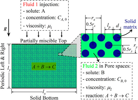
FIGURE 2. Schematic of the problem: density fingering with the reaction A + B → C in porous media.

Here, k is the kinetic reaction constant. All three chemical species contribute to fluid density and viscosity changes as follows [13, 14]:

$\rho ={\rho }_0+{\rho }_0\left({\beta }_A{C}_A+{\beta }_B{C}_B+{\beta }_C{C}_C\right),(47)$

$\mu ={\mu }_B\exp \left(\frac{C_A}{C_{B,0}}{\text{R}}_A+\frac{C_C}{C_{B,0}}{\text{R}}_C\right),(48)$

where β_r is the concentration expansion coefficient of species r. ${\text{R}}_A=\ln \left({\mu }_A/{\mu }_B\right)$ and ${\text{R}}_C=\ln \left({\mu }_C/{\mu }_B\right)$ are log-to-viscosity ratios between pure solutions of species r at concentration C_r,0. Under the gravity field, the body force (or buoyancy force) is calculated as follows [37]:

$\mathit{F}={\rho }_0\mathit{g}\left({\beta }_A{C}_A+{\beta }_B{C}_B+{\beta }_C{C}_C\right).(49)$

Here, g is the acceleration vector of gravity. With such effects, different density stratifications develop, and density fingering may be triggered.

In this incompressible system, the thermal flow is not considered. Thus, fluid motion and species evolutions in pore spaces are described using Eqs 4–6. In addition, fluid density is fixed as ρ_l = ρ₀, the reaction source term is defined as S_r = a_rR_o, the heterogeneous reaction at the fluid–solid interface is not considered, and the three species are assumed to diffuse at the same rate D_r = D. For dimensionless parameters in Eq. 11, the characteristic length L, velocity U, concentration C_ch, and density ρ_ch are as follows:

$L=l_x,U=\sqrt{g{\beta }_{A}L{C}_{B,0}},C_{ch}=C_{B,0},{\rho }_{ch}={\rho }_0.(50)$

The Rayleigh numbers Ra_r and the Damköhler number Da are defined as follows:

${\text{Ra}}_r=\frac{g{\beta }_r{C}_{ch}{L}^3}{\nu D},{\text{Ra}}_{AB}=\frac{{\text{Ra}}_A}{{\text{Ra}}_B},{\text{Ra}}_{CB}=\frac{{\text{Ra}}_C}{{\text{Ra}}_B},\text{Da}=\frac{k{C}_{ch}L}{U}.(51)$

For such a problem, our recent works have studied fingering dynamics with effects of the reaction A + B → C and differential diffusion [37, 38]. Thus, in the following simulations, we introduce the impact of the three chemical species on fluid viscosity (Eq. 48) and seek to understand how the development of density fingering is affected. The Schmidt number and the Damköhler number are fixed as Sc = 100 and Da = 5, respectively, and different values of Ra_AB, Ra_CB, R_A, and R_C are selected to change test conditions. During LB simulations, the no-slip and no-flux bottom wall and matrix interface are realized using the halfway bounce-back scheme, periodic conditions are set at the two lateral boundaries, and the partially miscible top boundary is implemented using the non-equilibrium extrapolation scheme. The relaxation rates in this simulation case are set as follows: s₀ = s₃ = s₅ = 0, s₁ = 1.1, s₂ = 1.2, s₄ = s₆ = (16τ − 8)/(8τ − 1), s₇ = s₈ = 1/τ, s_r,0 = 1, s_r,1 = s_r,2 = 1.1, s_r,3 = s_r,4 = s_r,5 = s_r,6 = 1/τ_r, and s_r,7 = s_r,8 = 0.9. A mesh of N_x × N_y = 1,500 × 1,000 lattice size is used after grid convergence validations.

We focus on density fingering phenomena with fluid viscosity variations caused by chemical species. Simulations with Ra_AB = 1, Ra_CB = 1, R_A = 0, and different values of R_C are first performed. From our calculated results, different types of density fingering are identified, and fingering is found to be stabilized as C decreases the fluid viscosity (R_C < 0). To illustrate such effects, the results of three cases with R_C = −3, 0, 3 are provided and discussed. It should be noted that the three values of R_C represent the three different scenarios where the reaction product C decreases, cannot change, or increases the fluid viscosity, respectively. For each of the three cases, Figure 3 depicts density distributions at six time instants, with the dimensionless density being calculated as ρ* = (ρ − ρ₀)/(ρ₀β_BC_B,0). From the constant-viscosity case (R_C = 0) in Figures 3A,B, a classical density fingering development pattern is observed, that is, fluid diffusion, individual fingering growth, fingering merge, and new fingering reinitiation [37]. It should be noted that during the initial diffusion stage, dense fluid accumulates near the top boundary to overcome the viscous shear force blow. Fingering develops when the driving force introduced by the accumulated dense fluid is large enough.

FIGURE 3

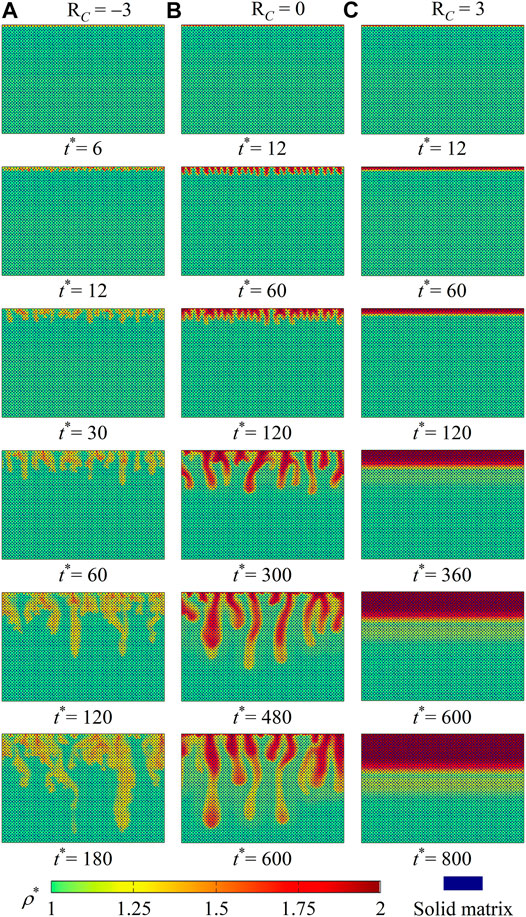
FIGURE 3. Density contours ρ* at six time instants for cases with Ra_AB = 1, Ra_CB = 1, and R_A = 0 and (A) R_C = −3, (B) R_C = 0, and (C) R_C = 3.

Compared with this constant-viscosity case, the introduction of viscosity variations in Figures 3A,C yields different density fingering dynamics. On one hand, when chemical product C decreases the fluid viscosity (Figure 3A with R_C = −3), the classical fingering development pattern is observed. However, fingering starts earlier and grows faster than in the constant-viscosity case (Figure 3B). Such an accelerated fingering propagation finally leads to diluted fingers. On the other hand, in the case with solute C increasing the fluid viscosity (Figure 3C with R_C = 3), even though the dissolution of A and the reaction A+ B → C can introduce a buoyantly unstable stratification, the fluid interface remains flat at each time instant, and no density fingering occurs.

In order to explain such influence of fluid viscosity variations, distributions of species concentrations ($C_r^{*}=C_r/C_{B,0}$) and fluid viscosity (μ* = μ/μ₂) are calculated and provided in Figure 4. For each case, results in Figure 4 correspond to the density field in Figure 3 at the last time instant. First, in the constant-viscosity case, Figure 4B shows that μ* distributes uniformly and density fingering is introduced by fingers of species A. Then, in the case with R_C = −3 (Figure 4A), fingers of A are also observed to be at the origin of density fingering. However, compared with the constant-viscosity case (Figure 4B), μ* (or fluid viscous force) decreases with the generation of C in the top layer. It implies that less A is required to accumulate near the top boundary to overcome the viscous force. Thus, fingers of A start earlier and develop faster in the top layer occupied with C. Finally, in Figure 4C with R_C = 3, the chemical product C increases the fluid viscosity and viscous force in the top area. Therefore, even though dissolved A accumulates to overcome the enlarged viscous force, the driving force introduced by the accumulation of A is still not large enough, and the fluid interface remains flat without fingering phenomena. These results explain the observations in Figure 3.

FIGURE 4

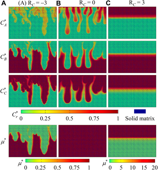
FIGURE 4. Contours of species concentrations $C_r^{*}$ and fluid viscosity μ* for cases with Ra_AB = 1, Ra_CB = 1, and R_A = 0 and (A) R_C = −3 at t* = 180, (B) R_C = 0 at t* = 600, and (C) R_C = 3 at t* = 600.

To quantitatively compare fingering dynamics in the three cases, Figure 5 plots temporal evolutions of the front position l_m/l_y, volume-averaged storage of A in the host fluid $⟨C_A^{*}+C_C^{*}⟩$, and horizontally averaged mass flux of A at the top boundary J*. Here, l_m is defined as the most advanced vertical position of density fingering in the host fluid, and J* is calculated as $J^{*}=-{\int }_0^{l_x^{*}}{\partial }_{y^{*}}{C}_A^{*}d{x}^{*}/(l_x^{*}\sqrt{{\text{Ra}}_B\text{Sc}})$. Curves of l_m/l_y show that the fingering front keeps growing in a diffusive tendency at R_C = 3, indicating the stable fluid interface. In the other two cases, however, l_m/l_y gradually departs from the diffusive tendency due to the onset of density fingering. Moreover, among the three cases, fingering at R_C = −3 propagates the fastest. This is because solute C decreases the fluid viscosity and destabilizes fingering development. Results of $⟨C_A^{*}+C_C^{*}⟩$ and J* also suggest that the decreased fluid viscosity at R_C = −3 accelerates the storage speed of A in the host fluid. Finally, by comparing the status of the three cases with l_m/l_y = 0.5, the stored amount of A is found to be the smallest in the case R_C = −3. This is attributed to the fact that the fast fingering propagation decreases the time period for the dissolution of A from the top boundary. These results quantitatively confirm the above fingering scenarios in Figure 3.

FIGURE 5

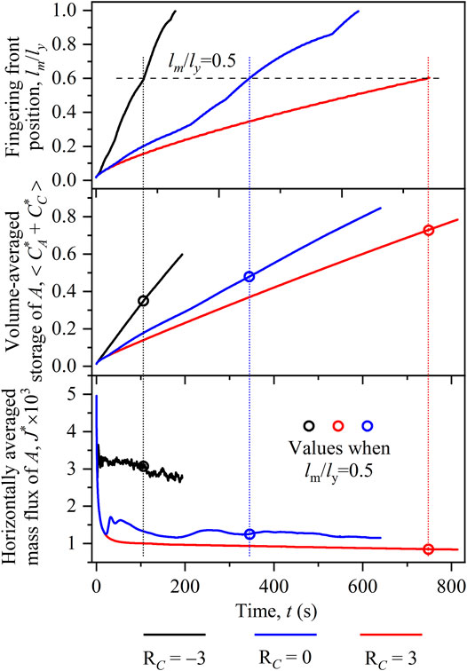
FIGURE 5. Temporal evolutions of (A) front position l_m/l_x, (B) volume-averaged storage of A in the host fluid $⟨C_A^{*}+C_C^{*}⟩$, and (C) horizontally averaged mass flux of A at the top boundary J* for cases with Ra_AB = 1, Ra_CB = 1, R_A = 0, and R_C = −3, 0, 3.

In general, when solute C decreases the fluid viscosity (R_C < 0), density fingering is destabilized, and the destabilizing intensity ascends with descending R_C. To further illustrate this impact, three cases with Ra_AB = 0.1 are conducted. Different from the above cases with Ra_AB = 1, the contribution to fluid density of A is smaller than that of B. Thus, in nonreactive cases, the unstable density contrast introduced by the dissolution of A from the top boundary is not large enough to bring in density fingering phenomena. As conducted in cases with Ra_AB = 1, Figures 6, 7 provide distributions of fluid density, species concentrations, and fluid viscosity. In the constant-viscosity case with Ra_CB = 1 and R_C = 0 (Figures 6B, 7B), the uniform fluid viscosity distribution and the flat fluid interface are observed. This indicates that the reaction A + B → C, without viscosity variations, cannot trigger the onset of density fingering. On the contrary, once the unstable viscosity contrast (R_C = −3) comes into play in the other two cases, density fingering appears and experiences the classical fingering development stages. First, in the case with Ra_CB = 1 and R_C = −3 (Figures 6A, 7A), the density contrast remains the same as in the constant-viscosity case (Figures 6B, 7B), but fluid viscosity in the top layer drops down with the generation of C. As a result, viscous force decreases and fluid mobility increases in the top area, which makes dissolved A grow in a finger-like shape and thus induces the development of density fingering. Second, in the case with Ra_CB = 0.1 and R_C = −3 (Figures 6C, 7C), a buoyantly stable density stratification develops with chemical reaction. Nevertheless, as illustrated in the zoom-in view, the fluid interface is distorted with time and finally becomes fingered. It is because the chemical product C decreases fluid viscosity in the top area and thus helps dissolved A develop into density fingering. These cases with a small density contrast suggest that decreased fluid viscosity with the chemical product C can destabilize or even trigger the development of density fingering.

FIGURE 6

FIGURE 6. Density contours ρ* at six time instants for cases with Ra_AB = 0.1 and R_A = 0 and (A) Ra_CB = 1, R_C = −3, (B) Ra_CB = 1, R_C = 0, and (C) Ra_CB = 0.1, R_C = −3.

FIGURE 7

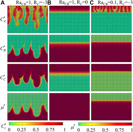
FIGURE 7. Contours of species concentrations $C_r^{*}$ and fluid viscosity μ* for cases with Ra_AB = 0.1 and R_A = 0 and (A) Ra_CB = 1, R_C = −3, at t* = 800, (B) Ra_CB = 1, R_C = 0, at t* = 900, and (C) Ra_CB = 0.1, R_CB = −3, at t* = 900.

4.2 Solid Coke Combustion With Viscous Fingering

The developed LB model is then applied to explore the solid coke combustion dynamics in porous media, which is a typical heterogeneous reaction at the interface between hot air and coke. As displayed in Figure 8, a 2D homogeneous structure with porosity ϕ = 0.406 is considered. The geometric parameters are set as l_x = 900 μm, l_y = 760 μm, d = 18 μm, δ = 3 μm, r_x = 42 μm, and r_y = 33 μm, respectively. Initially, solid coke is homogeneously deposited on unreactive solid matrices, and the pore spaces are filled with hot nitrogen at the temperature T₀ = 773 K. Then, hot air at the temperature T₀ and with the oxygen (O₂) mass fraction $Y_{{\text{O}}_2,0}=0.233$ is injected to react with coke by a driving force F = (F_x, 0). For simplicity, coke combustion is assumed to take place at the air–coke interface I as C + O₂ → CO₂ + Q [50]. The released heat is calculated using Q = R_eh_r, with h_r being the chemical reaction heat. The reaction rate R_e is estimated according to the first-order Arrheniust-type Eq. 39 as follows:

$R_e=A\exp \left(-E/RT\right)Y_{{\text{O}}_2}^I\rho /M_{{\text{O}}_2},(52)$

where A, E, and R are the pre-exponential factor, the activation energy, and the ideal gas constant, respectively. As for boundary conditions, zero-gradient conditions are applied for all the scalars at the outlet, and the top and the bottom are periodic. The impact of reaction heat and mass transfer on fluid viscosity is considered as follows [51]:

$\mu ={\mu }_2\exp \left({\text{R}}_y\frac{Y_{{\text{O}}_2}}{Y_{{\text{O}}_2,0}}+{\text{R}}_t\frac{T-T_0}{T_h-T_0}\right).(53)$

FIGURE 8

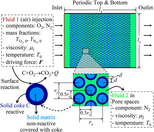
FIGURE 8. Schematic of the problem: coke combustion in porous media.

Here, ${\text{R}}_y=\ln \left({\mu }_1/{\mu }_2\right)$ and ${\mathrm{R}}_t=\ln \left({\mu }_{T_h}/{\mu }_2\right)$ are the mass and thermal viscosity ratios, respectively. μ₁ and μ₂ are viscosities of fluids 1 and 2 at T = T₀, respectively. ${\mu }_{T_h}$ is the viscosity of fluid 2 at T = T_h.

For this case, fluid flow and species evolutions in pore spaces, as well as heat transfer in both pores and solid phases are described using Eqs 4–7. The reaction source term is set as S_r = 0 because homogeneous reaction is not involved. On the other hand, coke combustion is described using Eqs 8–10 and implemented using the bounce-back scheme in Eqs 44, 45. The conversion between physical and lattice units is based on dimensionless parameters in Eq. 11 and the characteristic parameters are selected as L = 0.5r_x, U = α_l/L, ρ_ch = ρ_l,0, and T_ch = 3,000 K [39]. In the subsequent simulations, the required parameters are set as A = 9.717 × 10⁶ m/s, E = 131.09 kJ/mol, hr = 388.5 kJ/mol, ρ_sc_p,s/ρ_lc_p,l = 368, and α_s/α_g = 0.119, respectively. The Reynolds, Prandtl, and Peclet numbers are fixed as Re = 1.4, Pr = 0.7, and Pe = 1.5, the driving force is $F_x^{*}=7.3$, and a mesh of size N_x × N_y = 900 × 760 is used after grid convergence tests. In addition, the relaxation rates used in this case are as follows: s₀ = s₃ = s₅ = 1, s₁ = s₂ = 0.9, s₄ = s₆ = (16τ − 8)/(8τ − 1), s₇ = s₈ = 1/τ, s_r,0 = 1, s_r,1 = s_r,2 = 1.1, s_r,3 = s_r,4 = s_r,5 = s_r,6 = 1/τ_r, s_r,7 = s_r,8 = 0.9, s_T,0 = 1, s_T,1 = s_T,2 = 1.1, s_T,3 = s_T,4 = s_T,5 = s_T,6 = 1/τ_T, and s_T,7 = s_T,8 = (16τ_T − 8)/(8τ_T − 1).

Our recent work has investigated the general coke combustion dynamics and evaluated the key influencing conditions, with the fluid viscosity being assumed to be a constant [39]. In practical applications, however, fluid viscosity varies with heat and mass transfer. Therefore, this work extends to studying the impact of viscosity variations on the combustion front stability. A base case with R_y = 0 and R_t = 0 is simulated at first. Figure 9 illustrates the distributions of residual coke, O₂ mass fraction $Y_{{\text{O}}_2}$, and temperature T/T₀ at the time instant t = 5.62 s. As can be seen, the combustion front extends around a grain diameter. In this area, coke and O₂ are fully consumed by combustion, and the combustion front remains flat without fingering phenomena. Furthermore, temperature is observed to increase from the inlet and then reaches a peak value at the combustion front and finally drops to T₀ on the downstream side. This distribution is attributed to the released combustion heat at the combustion front. It is also noticed that fluid on the downstream side (i.e., the area from the combustion front to the outside) is slightly hotter than that on the upstream side. This is caused by both the flow direction and the heat transfer that is faster than the combustion front movement [39]. In this case, the coke combustion with the stable combustion front, low temperature increase, and full coke and O₂ utilization rate can fit engineering requirements.

FIGURE 9

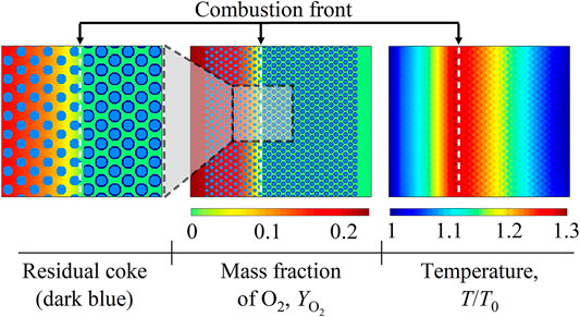
FIGURE 9. Contours of residual coke, the O₂ mass fraction $Y_{{\text{O}}_2}$, and temperature T/T₀ for the base case with R_y = 0 and R_t = 0 at t = 5.62 s.

The fluid viscosity remains uniform in the above base case. Thus, two cases with R_y = −4, R_t = 0 and R_y = −4, R_t = −3 are then considered. Other simulation parameters are set to be the same as in the base case, except for the Peclet number Pe = 10. Spatial distributions of residual coke, the O₂ mass fraction $Y_{{\text{O}}_2}$, and temperature T/T₀ for the two cases are provided in Figure 10. Results show that in each of the two cases with R_y = −4, the combustion front proceeds in a finger-like pattern along the x direction. This is different from the flat combustion front in the base case (Figure 9), implying the destabilizing effects of the viscosity contrast R_y = −4. As for the temperature field, the maximum temperature occurs at the combustion front as in the base case. However, compared with the base case, the combustion fronts in these two cases are decelerated, and the temperature of the downstream side is no longer obviously higher than that of the upstream side. This is because the highly viscous fluid on the downstream side prevents the fluid propagation and thus slows down both the front movement and the heat transfer.

FIGURE 10

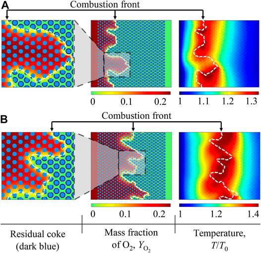
FIGURE 10. Contours of residual coke, the O₂ mass fraction $Y_{{\text{O}}_2}$, and temperature T/T₀ for the two cases at t = 8.14 s with (A) R_y = 4, R_t = 0 and (B) R_y = 4, R_t = −3.

In the case with R_t = −3, the fluid viscosity decreases with the increasing temperature. By comparing results in Figures 10A,B, such temperature-induced viscosity variations are found to influence coke combustion properties. On one hand, the fluid prorogation along the x direction is accelerated and more fingers at the combustion front are triggered. This destabilizing impact is attributed to the fact that combustion heat is released to increase the local temperature and decrease the fluid viscosity at the combustion front. Subsequently, the unstable viscosity contrast between fluids at the combustion front and on the downstream side is enlarged, which enhances viscous fingering phenomena. On the other hand, the combustion front temperature increases. It is explained by the fact that in the combustion front area, the high temperature induces the low fluid viscosity and the accelerated fluid flow velocity. Subsequently, the injected O₂ can easily expand to react with coke and release heat, which leads to the increased combustion front temperature.

To further quantify differences between the two cases with viscosity variations, temporal evolutions of the volume-averaged temperature T_v/T₀ and the residual coke ratio Vr_c are calculated and illustrated in Figure 11. As can be seen, each line of Vr_c decreases with time because coke burns out gradually, while every temperature curve shows an increasing pattern due to the released combustion heat. In addition, the inclusion of temperature-induced viscosity variations is found to bring in high burning temperature and fast coke consumption. It is due to the fact that the increased front temperature brings in the decreased fluid viscosity and, hence, the enhanced coke combustion intensity. This quantitatively verifies the above observations in Figure 10. It should be emphasized that these two cases feature finger-like combustion fronts. They are thus undesirable in practical applications because the downstream fluid cannot be efficiently displaced.

FIGURE 11

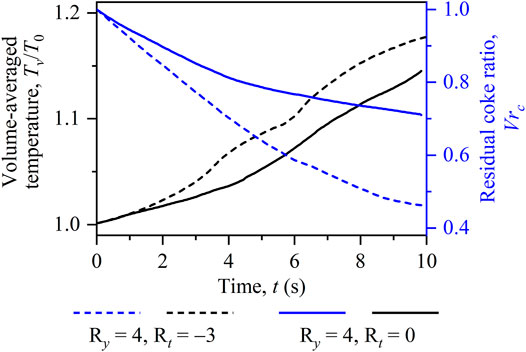
FIGURE 11. Temporal evolutions of the volume-averaged temperature T_v/T₀ and the residual coke ratio Vr_c for the two cases with R_y = 4, R_t = 0 and R_y = 4, R_t = −3.

5 Conclusion

Flows of reactive fluids in porous media have been studied on the pore scale. A multicomponent multiple-relaxation-time lattice Boltzmann (LB) model is developed to describe fluid motions and species evolutions in pore spaces, as well as heat transfer in both void pores and the solid phase. In the present model, separate LB equations are built to describe fluids and species evolutions during homogeneous reaction between miscible fluids; source terms and boundary schemes are derived to account for heterogeneous reaction at the fluid–solid interface; and additional correlation terms are introduced to model both incompressible and compressible (with temperature-dependent fluid density) fluid flows. Based on this model, two types of physical problems are simulated. One is density fingering with the homogeneous reaction A + B → C. Results show that depending on variations in the fluid viscosity caused by the chemical product C, the development of density fingering can be enhanced, suppressed, or even triggered. To further study effects of thermal flows, solid coke combustion in porous media is carried out. Simulation results successfully capture coke combustion dynamics and the evolution of the porous structure. Furthermore, the viscosity contrast caused by heat and mass transfer is found to change the coke combustion stability considerably. These two cases verify the capability of the proposed LB model in resolving flows of reactive fluids and the coupled viscosity and density instabilities on the pore scale. Extension to 3D porous media flows with chemical reaction is currently underway. The results are expected to clarify the differences and similarities between 2D and 3D simulations.

Data Availability Statement

The raw data supporting the conclusion of this article will be made available by the authors, without undue reservation.

Author Contributions

TL has conducted the research while KL has supervised the project, with regular discussions with each other. Both authors have contributed to the writing of the manuscript.

Funding

This work was supported by the UK Engineering and Physical Sciences Research Council under grant nos. EP/R029598/1 and EP/S012559/1 and the China Scholarship Council (CSC) under grant no. 201706160161.

Conflict of Interest

The authors declare that the research was conducted in the absence of any commercial or financial relationships that could be construed as a potential conflict of interest.

The handling editor declared a past co‐authorship with one of the authors KL.

Publisher’s Note

All claims expressed in this article are solely those of the authors and do not necessarily represent those of their affiliated organizations, or those of the publisher, the editors, and the reviewers. Any product that may be evaluated in this article, or claim that may be made by its manufacturer, is not guaranteed or endorsed by the publisher.

Acknowledgments

The PhD scholarship for TL from the UCL Mechanical Engineering Department is gratefully acknowledged.

References

1. Stevens JD, Sharp JM, Simmons CT, Fenstemaker TR. Evidence of Free Convection in Groundwater: Field-Based Measurements Beneath Wind-Tidal Flats. J Hydrol (2009) 375:394–409. doi:10.1016/j.jhydrol.2009.06.035

CrossRef Full Text | Google Scholar

2. Cardoso SS, Andres JT. Geochemistry of Silicate-Rich Rocks Can Curtail Spreading of Carbon Dioxide in Subsurface Aquifers. Nat Commun (2014) 5:5743–6. doi:10.1038/ncomms6743

PubMed Abstract | CrossRef Full Text | Google Scholar

3. Rongy L, Haugen KB, Firoozabadi A. Mixing from Fickian Diffusion and Natural Convection in Binary Non-Equilibrium Fluid Phases. Aiche J (2012) 58:1336–45. doi:10.1002/aic.12685

CrossRef Full Text | Google Scholar

4. Jiang XZ, Luo KH, Ventikos Y. Principal Mode of Syndecan-4 Mechanotransduction for the Endothelial Glycocalyx Is a Scissor-Like Dimer Motion. Acta Physiol (Oxf) (2020) 228:e13376. doi:10.1111/apha.13376

PubMed Abstract | CrossRef Full Text | Google Scholar

5. He Y-L, Liu Q, Li Q, Tao W-Q. Lattice Boltzmann Methods for Single-Phase and Solid-Liquid Phase-Change Heat Transfer in Porous Media: A Review. Int J Heat Mass Transf (2019) 129:160–97. doi:10.1016/j.ijheatmasstransfer.2018.08.135

CrossRef Full Text | Google Scholar

6. De Wit A. Chemo-Hydrodynamic Patterns and Instabilities. Annu Rev Fluid Mech (2020) 52:531–55. doi:10.1146/annurev-fluid-010719-060349

CrossRef Full Text | Google Scholar

7. Budroni MA, Riolfo LA, Lemaigre L, Rossi F, Rustici M, De Wit A. Chemical Control of Hydrodynamic Instabilities in Partially Miscible Two-Layer Systems. J Phys Chem Lett (2014) 5:875–81. doi:10.1021/jz5000403

PubMed Abstract | CrossRef Full Text | Google Scholar

8. Thomas C, Loodts V, Rongy L, De Wit A. Convective Dissolution of CO 2 in Reactive Alkaline Solutions: Active Role of Spectator Ions. Int J Greenh Gas Control (2016) 53:230–42. doi:10.1016/j.ijggc.2016.07.034

CrossRef Full Text | Google Scholar

9. Cherezov I, Cardoso SSS. Acceleration of Convective Dissolution by Chemical Reaction in a Hele-Shaw Cell. Phys Chem Chem Phys (2016) 18:23727–36. doi:10.1039/c6cp03327j

PubMed Abstract | CrossRef Full Text | Google Scholar

10. Wylock C, Rednikov A, Colinet P, Haut B. Experimental and Numerical Analysis of Buoyancy-Induced Instability During CO₂ Absorption in NaHCO₃-Na₂CO₃ Aqueous Solutions. Chem Eng Sci (2017) 157:232–46. doi:10.1016/j.ces.2016.04.061

CrossRef Full Text | Google Scholar

11. Loodts V, Trevelyan PM, Rongy L, De Wit A. Density Profiles Around A+B→C Reaction-Diffusion Fronts in Partially Miscible Systems: A General Classification. Phys Rev E (2016) 94:043115. doi:10.1103/PhysRevE.94.043115

PubMed Abstract | CrossRef Full Text | Google Scholar

12. Trevelyan PM, Almarcha C, De Wit A. Buoyancy-Driven Instabilities Around Miscible A+B→C Reaction Fronts: a General Classification. Phys Rev E Stat Nonlin Soft Matter Phys (2015) 91:023001. doi:10.1103/PhysRevE.91.023001

PubMed Abstract | CrossRef Full Text | Google Scholar

13. Hejazi SH, Trevelyan PMJ, Azaiez J, De Wit A. Viscous Fingering of a Miscible Reactive A + B → C Interface: a Linear Stability Analysis. J Fluid Mech (2010) 652:501–28. doi:10.1017/s0022112010000327

CrossRef Full Text | Google Scholar

14. Loodts V, Knaepen B, Rongy L, De Wit A. Enhanced Steady-State Dissolution Flux in Reactive Convective Dissolution. Phys Chem Chem Phys (2017) 19:18565–79. doi:10.1039/c7cp01372h

PubMed Abstract | CrossRef Full Text | Google Scholar

15. Loodts V, Saghou H, Knaepen B, Rongy L, De Wit A. Differential Diffusivity Effects in Reactive Convective Dissolution. Fluids (2018) 3:83. doi:10.3390/fluids3040083

CrossRef Full Text | Google Scholar

16. Nagatsu Y, De Wit A. Viscous Fingering of a Miscible Reactive A+B→C Interface for an Infinitely Fast Chemical Reaction: Nonlinear Simulations. Phys Fluids (2011) 23:043103. doi:10.1063/1.3567176

CrossRef Full Text | Google Scholar

17. Szymczak P, Ladd AJC. Reactive-infiltration Instabilities in Rocks. Part 2. Dissolution of a Porous Matrix. J Fluid Mech (2014) 738:591–630. doi:10.1017/jfm.2013.586

CrossRef Full Text | Google Scholar

18. Szymczak P, Ladd AJC. Reactive-infiltration Instabilities in Rocks. Fracture Dissolution. J Fluid Mech (2012) 702:239–64. doi:10.1017/jfm.2012.174

CrossRef Full Text | Google Scholar

19. Fredd CN, Fogler HS. Influence of Transport and Reaction on Wormhole Formation in Porous Media. Aiche J (1998) 44:1933–49. doi:10.1002/aic.690440902

CrossRef Full Text | Google Scholar

20. Menke HP, Bijeljic B, Blunt MJ. Dynamic Reservoir-Condition Microtomography of Reactive Transport in Complex Carbonates: Effect of Initial Pore Structure and Initial Brine Ph. Geochim Cosmochim Acta (2017) 204:267–85. doi:10.1016/j.gca.2017.01.053

CrossRef Full Text | Google Scholar

21. Nagatsu Y, Ishii Y, Tada Y, De Wit A. Hydrodynamic Fingering Instability Induced by a Precipitation Reaction. Phys Rev Lett (2014) 113:024502. doi:10.1103/PhysRevLett.113.024502

PubMed Abstract | CrossRef Full Text | Google Scholar

22. Haudin F, De Wit A. Patterns Due to an Interplay Between Viscous and Precipitation-Driven Fingering. Phys Fluids (2015) 27:113101. doi:10.1063/1.4934669

CrossRef Full Text | Google Scholar

23. Hao Y, Smith MM, Carroll SA. Multiscale Modeling of CO2-Induced Carbonate Dissolution: From Core to Meter Scale. Int J Greenh Gas Control (2019) 88:272–89. doi:10.1016/j.ijggc.2019.06.007

CrossRef Full Text | Google Scholar

24. Golfier F, Zarcone C, Bazin B, Lenormand R, Lasseux D, Quintard M. On the Ability of a Darcy-Scale Model to Capture Wormhole Formation during the Dissolution of a Porous Medium. J Fluid Mech (2002) 457:213–54. doi:10.1017/s0022112002007735

CrossRef Full Text | Google Scholar

25. Panga MKR, Ziauddin M, Balakotaiah V. Two-scale Continuum Model for Simulation of Wormholes in Carbonate Acidization. Aiche J (2005) 51:3231–48. doi:10.1002/aic.10574

CrossRef Full Text | Google Scholar

26. Sabet N, Mohammadi M, Zirahi A, Zirrahi M, Hassanzadeh H, Abedi J. Numerical Modeling of Viscous Fingering During Miscible Displacement of Oil by a Paraffinic Solvent in the Presence of Asphaltene Precipitation and Deposition. Int J Heat Mass Transf (2020) 154:119688. doi:10.1016/j.ijheatmasstransfer.2020.119688

CrossRef Full Text | Google Scholar

27. Sabet N, Hassanzadeh H, Abedi J. Dynamics of Viscous Fingering in Porous Mdia in the Presence of In Situ Formed Precipitates and Their Subsequent Deposition. Water Resour Res (2020) 56:e2019WR027042. doi:10.1029/2019wr027042

CrossRef Full Text | Google Scholar

28. Guo K, Li H, Yu Z. In-Situ Heavy and Extra-Heavy Oil Recovery: A Review. Fuel (2016) 185:886–902. doi:10.1016/j.fuel.2016.08.047

CrossRef Full Text | Google Scholar

29. Zhu ZY. Efficient Simulation of thermal Enhanced Oil Recovery Processes. Stanford, California, USA: Ph.D. thesis, Stanford University (2011).

30. Srinivasareddy D, Kumar GS. A Numerical Study on Phase Behavior Effects in Enhanced Oil Recovery by In Situ Combustion. Pet Sci Technology (2015) 33:353–62. doi:10.1080/10916466.2014.979999

CrossRef Full Text | Google Scholar

31. Zheng H, Shi WP, Ding DL, Zhang CY. Numerical Simulation of In Situ Combustion of Oil Shale. Geofluids (2017) 2017. doi:10.1155/2017/3028974

CrossRef Full Text | Google Scholar

32. Xu Q, Long W, Jiang H, Zan C, Huang J, Chen X, et al. Pore-Scale Modelling of the Coupled Thermal and Reactive Flow at the Combustion Front During Crude Oil In-Situ Combustion. Chem Eng J (2018) 350:776–90. doi:10.1016/j.cej.2018.04.114

CrossRef Full Text | Google Scholar

33. Li Q, Luo KH, Kang QJ, He YL, Chen Q, Liu Q. Lattice Boltzmann Methods for Multiphase Flow and Phase-Change Heat Transfer. Prog Energ Combust Sci (2016) 52:62–105. doi:10.1016/j.pecs.2015.10.001

CrossRef Full Text | Google Scholar

34. Guo Z, Shu C. Lattice Boltzmann Method and its Applications in Engineering. Singapore, Singapore: World Scientific Publisher (2013). Vol. 3, p. 25–8.

35. Zhang L, Zhang C, Zhang K, Zhang L, Yao J, Sun H, et al. Pore‐Scale Investigation of Methane Hydrate Dissociation Using the Lattice Boltzmann Method. Water Resour Res (2019) 55:8422–44. doi:10.1029/2019wr025195

CrossRef Full Text | Google Scholar

36. Lei T, Meng X, Guo Z. Pore-scale Study on Reactive Mixing of Miscible Solutions With Viscous Fingering in Porous media. Comput Fluids (2017) 155:146–60. doi:10.1016/j.compfluid.2016.09.015

CrossRef Full Text | Google Scholar

37. Lei T, Luo KH. Pore-Scale Study of Dissolution-Driven Density Instability With Reaction A + B → C in Porous media. Phys Rev Fluids (2019) 4:063907. doi:10.1103/physrevfluids.4.063907

CrossRef Full Text | Google Scholar

38. Lei TM, Luo KH. Differential Diffusion Effects on Density-Driven Instability of Reactive Flows in Porous Media. Phys Rev Fluids (2020) 5:033903. doi:10.1103/physrevfluids.5.033903

CrossRef Full Text | Google Scholar

39. Lei T, Wang Z, Luo KH. Study of Pore-Scale Coke Combustion in Porous Media Using Lattice Boltzmann Method. Combust Flame (2021) 225:104–19. doi:10.1016/j.combustflame.2020.10.036

CrossRef Full Text | Google Scholar

40. Lei T, Luo KH. Pore-Scale Simulation of Miscible Viscous Fingering With Dissolution Reaction in Porous Media. Phys Fluids (2021) 33:034134. doi:10.1063/5.0045051

CrossRef Full Text | Google Scholar

41. Kang Q, Chen L, Valocchi AJ, Viswanathan HS. Pore-Scale Study of Dissolution-Induced Changes in Permeability and Porosity of Porous media. J Hydrol (2014) 517:1049–55. doi:10.1016/j.jhydrol.2014.06.045

CrossRef Full Text | Google Scholar

42. d’Humieres D. Multiple-Relaxation-Time Lattice Boltzmann Models in Three Dimensions. Philosophical Trans R Soc Lond Ser A: Math Phys Eng Sci (2002) 360:437–51. doi:10.1098/rsta.2001.0955

Google Scholar

43. Guo Z, Zheng C. Analysis of Lattice Boltzmann Equation for Microscale Gas Flows: Relaxation Times, Boundary Conditions and the Knudsen Layer. Int J Comput Fluid Dyn (2008) 22:465–73. doi:10.1080/10618560802253100

CrossRef Full Text | Google Scholar

44. Lallemand P, Luo L-S. Theory of the Lattice Boltzmann Method: Dispersion, Dissipation, Isotropy, Galilean Invariance, and Stability. Phys Rev E (2000) 61:6546–62. doi:10.1103/physreve.61.6546

CrossRef Full Text | Google Scholar

45. Karani H, Huber C. Lattice Boltzmann Formulation for Conjugate Heat Transfer in Heterogeneous media. Phys Rev E Stat Nonlin Soft Matter Phys (2015) 91:023304. doi:10.1103/PhysRevE.91.023304

PubMed Abstract | CrossRef Full Text | Google Scholar

46. Li Q, Luo KH, He YL, Gao YJ, Tao WQ. Coupling Lattice Boltzmann Model for Simulation of Thermal Flows on Standard Lattices. Phys Rev E Stat Nonlin Soft Matter Phys (2012) 85:016710. doi:10.1103/PhysRevE.85.016710

PubMed Abstract | CrossRef Full Text | Google Scholar

47. Feng Y, Tayyab M, Boivin P. A Lattice-Boltzmann Model for Low-Mach Reactive Flows. Combust Flame (2018) 196:249–54. doi:10.1016/j.combustflame.2018.06.027

CrossRef Full Text | Google Scholar

48. Guo Z, Zheng C, Shi B. Force Imbalance in Lattice Boltzmann Equation for Two-phase Flows. Phys Rev E Stat Nonlin Soft Matter Phys (2011) 83:036707. doi:10.1103/PhysRevE.83.036707

PubMed Abstract | CrossRef Full Text | Google Scholar

49. Zhang T, Shi B, Guo Z, Chai Z, Lu J. General Bounce-Back Scheme for Concentration Boundary Condition in the Lattice-Boltzmann Method. Phys Rev E Stat Nonlin Soft Matter Phys (2012) 85:016701. doi:10.1103/PhysRevE.85.016701

PubMed Abstract | CrossRef Full Text | Google Scholar

50. Mailybaev AA, Bruining J, Marchesin D. Analysis of In Situ Combustion of Oil With Pyrolysis and Vaporization. Combust Flame (2011) 158:1097–108. doi:10.1016/j.combustflame.2010.10.025

CrossRef Full Text | Google Scholar

51. Mishra M, Trevelyan PMJ, Almarcha C, De Wit A. Influence of Double Diffusive Effects on Miscible Viscous Fingering. Phys Rev Lett (2010) 105:204501. doi:10.1103/physrevlett.105.204501

PubMed Abstract | CrossRef Full Text | Google Scholar