- 1Naval Research Laboratory, Washington, DC, United States
- 2UMBC, Baltimore, MD, United States
- 3Heliophysics Science Division, NASA/Goddard Space Flight Center, Greenbelt, MD, United States
- 4MC 672, GSFC/NASA, Greenbelt, MD, United States
- 5IFIR/UNR-CONICET, Rosario, Argentina
We describe a new NASA website that shows normalized magnetic field (B) magnitude profiles within Wind magnetic clouds (MCs) (i.e., observations versus basic model versus modified model) for 209 MCs observed from launch in late 1994 to July of 2015, where model modification is based on the studies of Lepping et al. (Solar Phys, 2017, 292:27) and Lepping et al. (Solar Phys, 2018, 293:162); the basic force free magnetic cloud parameter fitting model employing Bessel functions (Lepping et al., J. Geophys. Res., 1990, 95:11957) is called the LJB model here. The fundamental principles should be applicable to the B-data from any spacecraft at 1 AU. Earlier (in the LJB study), we justified why the field magnitude can be thought of as decoupled from the field direction within an MC, and further, we justified this idea in terms of actual observations seen over a few decades with examples of MCs from Wind data. The model modification is achieved by adding a correction (“Quad”) value to the LJB model (Bessel function) value in the following manner: B (est)/B0 ≈ [LJB Model + Quad (CA,u)], where B0 is the LJB-estimated field magnitude value on the MC’s axis, CA is the relative closest approach (See Supplementary Appendix A), and u is the distance that the spacecraft travels through the MC from its entrance point. In an average sense, the Quad technique is shown to be successful for 82% of the past modeled MCs, when Quality (Q0) is good or excellent (see Supplementary Appendix A). The Quad technique is successful for 78% of MCs when all cases are considered. So Q0 of the MC LJB-fit is not a big factor when the success of the Quad scheme is considered. In addition, it is found that the Quad technique does not work better for MC events with higher solar wind speed. Yearly occurrence frequency of all MC events (NYearly) and those MC events with ΔσN/σN2 ≥ 0.5 (NΔσN/σN2≥0.5) are well correlated, but there is no solar cycle dependence for normalizing NΔσN/σN2≥0.5 with NYearly.
1 Introduction and Background
A magnetic cloud (MC) is a solar wind region with the following features: enhanced magnetic field strength, a smooth change in magnetic field direction as observed by a spacecraft passing through the MC, low proton temperature compared to the ambient proton temperature, and low proton plasma beta (e.g., [1–3]). Also, we must require that the duration of the MC be 5 h or more, based on numerous observations. Many MC lists are available (e.g., [4–11]). Enhanced southward magnetic field of an MC will cause geomagnetic activity while the MC is passing by the Earth. Here, we call attention to a method of modifying a normalized magnetic field (B) magnitude profile within a Wind magnetic cloud (MC) (or for any spacecraft at 1 AU) by describing a new website that shows B-profiles (observations vs. model vs. modified model) for 209 cases of Wind MCs from launch (late 1994) to the end of 2015. The model modification is based on the studies of Lepping et al. [12] and Lepping et al. [10]; the basic MC parameter fitting (force free) model is that of Lepping et al. [13] (henceforth called the LJB model). The modification is based on the statistics of many actual MCs observed in the past by the Wind spacecraft. (For articles on the discovery of MCs and other relevant aspects see [1–3].)
The justification for separating the magnitude of B from its direction in the implementation of the LJB model results from the manner in which the model was posed in the first place and in what was shown to be the characteristics of hundreds of actual MCs from many different spacecraft. That is, the model always operated on the fundamental assumption that we could unit-normalize B (i.e., create B/|B| at all points) within the MC and carry out the least-square fitting of the model to the resulting data, being the unit normalized-B—not on the actual B. And only later do we adjust the B (model) profile to the average value of B across the MC; this leads to providing an appropriate B0, which is the estimated value for the magnetic field magnitude on the axis of the MC. In particular, this treatment for over 200 Wind MCs has generally provided a faithful reproduction of the profile of the direction of B within a MC for most cases (i.e., at least at 1 AU) and especially when considering the lower frequency components of B, that is, excluding what may be considered “noise.” But the model rarely gives a very good reproduction of the actual profile of the magnitude of B. The study by Lepping et al. [10] attempts to statistically correct for this shortcoming of the LJB model, as described below.
2 The Quad Scheme for Modifying the B-Intensity Within the Magnetic Cloud
Recently, a scheme was developed by Lepping et al. [10] to provide a more realistic B/B0 profile of an MC, than that used in the LJB model, based on the results of 21 years of MCs studied from the Wind spacecraft (also, see Lepping et al. [10,12] for more detail on the foundation of the scheme). It was shown statistically that this scheme should improve MC profiles by about 82% of the time, when the highest quality (Q0) MCs are considered. Q0 can take one of three possible values: 1 (excellent), 2 (good/fair), and 3 (poor) (see Supplementary Appendix A, for a strict definition of Q0). To provide differing examples, Figure 1 shows plots of B/B0 versus %-of-time through the MC for three MCs (cases of #s 70, 71, and 62, all of Q0 = 1), in terms of actual observations (101 averages across each MC, i.e., data averaged into 100 bins across each MC shown by the dot-dot-dashed curve; called the Obs curve), the original Bessel function model profile (the black solid-line curve, described by LJB), and the new statistically modified version (the red dashed curve, described generically by Lepping et al., 2018). MC #70 starts on 2002-03-24, #71 starts on 2002-04-18, and #62 starts on 2001-04-12; these dates are shown on the first line at the top of each panel of Figure 1. Also, within each panel of the figure are the start time (also on the first line at the top), and then the value of the relative closest approach in percentage (CA ≡ |Y0|/R0 in %), Q0, the MC duration (τ), the average plasma speed within the MC (<VMC>), and the estimated B0, where Y0 is the closest approach and R0 is the estimated radius of the MC. Below the curves is the quantity ΔσN/σN2 described by Lepping et al. [10] as a good measure of how well the scheme is performing; when ΔσN/σN2 is above 0.5, it is doing very well (or exceptional when it approaches or exceeds 1.0); when it is between 0.0 and 0.5, it is acceptable; when it is negative, it is a failure. We give an abbreviated interpretation of ΔσN/σN2 here as follows:
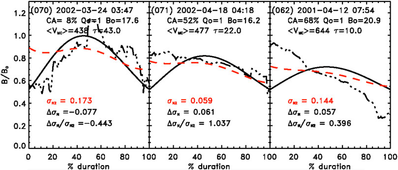
FIGURE 1. Three examples (the cases of #s 70, 71, and 62 of Wind MCs; see the associated starting dates of these MCs on the first line at the top of each panel) of plots of B/B0-profiles: B0-normalized B observations (black dash-dot-dot), force free model values (black solid curve) and modified-model values (red dashed curve from Lepping et al. [10]—all as a function of percent passage through the MC (i.e., u in %); each profile has 101 points across. In each panel the following are shown: TOP OF EACH PANEL: the start time (year-month-day of month) hour:minute (UT), CA (= |Y0|/R0 in %), Quality (Q0), B0 (in nT), average plasma speed within the MC (<VMC>, in km s−1), and duration (τ, in hours), BOTTOM OF EACH PANEL: the values of the quantities ΔσN ,σN2, and ΔσN/σN2 (see text) that are described by Lepping et al. [10]. The ratio ΔσN/σN2 in particular is shown to be a good measure of how well the scheme is performing in general.
The ratio ΔσN/σN2 is a relative measure of the improvement in the B/B0 fit to the MC’s profile by using a so-called Quad (CA,u) formula weighted by the “accuracy” of the final fit, for the LJB model, where σN2 is a quantitative measure of how well the Quad equations fit the difference-profile between the observations and the model values; u is the distance measured as the spacecraft travels through the MC. ΔσN is a quantitative measure of the improvement in the fit of B/B0 after adding in the Quad modification (and ΔσN must be greater than or equal to 0.0 for a success), where B (est)/B0 ≈ [LJB Model + Quad (CA,u)], developed for four possible CAs (in%), 12.5, 37.5, 62.5, and 87.5 (these are the center points of four equally spaced segments of the full span of CA (0–100%)). Quad is a quadratic fit to the difference-quantity [B/B0(Observations)-LJB Model] for each point in the MC carried out statistically from 124 averaged (good quality, i.e., Q0 = 1,2) MCs using Wind B-data (see Lepping et al. [10] for a more detailed explanation of the ratio ΔσN/σN2).
Concerning specifics of the three examples of Figure 1, we note the following:
• For case #70, we have a ΔσN/σN2 = −0.443, a poor (negative) case, with a CA of 8% and a long duration of 43.0 h. Since the Quad technique usually works best when B/B0(Observations) is higher than the Bessel force free field in the early hours of the MC, which is not the case here, the “correction” field (red dashed curve in Figure 1) is too high in this case. This is a somewhat unusual case because of the low intensity field in these early hours, and therefore, it violates the assumptions on which the Quad technique was based and not surprisingly gives poor results, that is, the negative ratio for ΔσN/σN2 of -0.443, even though Q0 = 1. In fact, there usually is not a good correlation between ΔσN/σN2 and Q0 (see Figure 2 and related text (Section 5) concerning this issue). And finally, notice that Bo is 17.6 nT, a typical value for Bo, and <V> = 438 km s−1.
• For case #71 we have a ΔσN/σN2 = 1.037, an excellent case, with a CA of 52% and a fairly typical duration of 22.0 h. Here the observations are higher than the Bessel force free field (red dashed curve in Figure 1) in the early hours, which, as stated above is typical, and, in fact, this is an excellent example of such front-end enhancement in the field. Also Q0 = 1. Bo is 16.2 nT, another typical value for Bo, and finally, <V> = 477 km s−1.
• For case #62 with a ΔσN/σN2 = 0.396, we have an acceptable (intermediate) case, that is, a positive ratio but less than 0.500—and a short duration of the MC of 10 h. Here CA was moderately large (68%) and again Q0 = 1. Bo is 20.9 nT, a somewhat high value for Bo, and finally, a moderately high <V> = 644 km s−1.
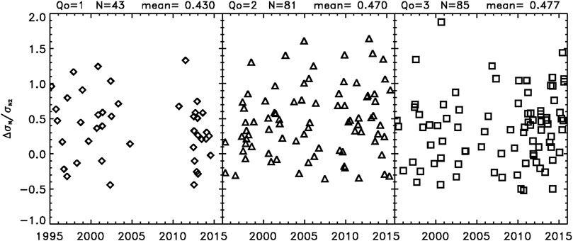
FIGURE 2. A plot of ΔσN/σN2 versus time for the family of Q0, showing almost the same average of ΔσN/σN2 for each Q0 (the averages are given above each panel), where Q0 = 1 set is represented by diamonds, Q0 = 2 by triangles, and Q0 = 3 by squares, with a large spread in values in each case.
All three cases were deliberately chosen to be in the Q0 = 1 category so that Quality would not be an obvious determinate in the value of the ratio ΔσN/σN2 (see comments in the Conclusions and Discussion (Section 5) about ΔσN/σN2 versus Q0).
3 Wind Website to Obtain the Full Set of Field Intensity Plots
The Website to obtain the MC B/Bo profiles is within the Wind/MFI Website, which is https://wind.nasa.gov/mfi/mag_cloud_pub1.html.
The link at that Website to the Field Intensity plots, based on the Quad scheme, is http://lepmfi.gsfc.nasa.gov/mfi/mag_cloud_B_magnitude.html.
Each MC has a case number (#) that is given (in parentheses) in the upper left-hand corner of each panel, as we saw in the three examples of Figure 1. We give below an example of a single page in the initial set.
4 Example of a Page of 20 Cases of Wind MCs
Figure 3 shows a single example page, that is, page 2, of a set of pages (20 panels each page, with one MC per panel) of the same quantities as shown in Figure 1 of Wind MCs from launch to July of 2015. A full set of 11 figures is shown in Supplementary Appendix B. Initially, there are 11 such pages in the Website described above, to cover the 209 MCs that are believed to exist over that period. Notice that the figure shows that the force free Bessel fields (solid black lines) at the start and end times, for all cases, give the same B/Bo value of about 0.52, as expected. The upper left-hand corner of each panel shows the case number (#) of the MC.
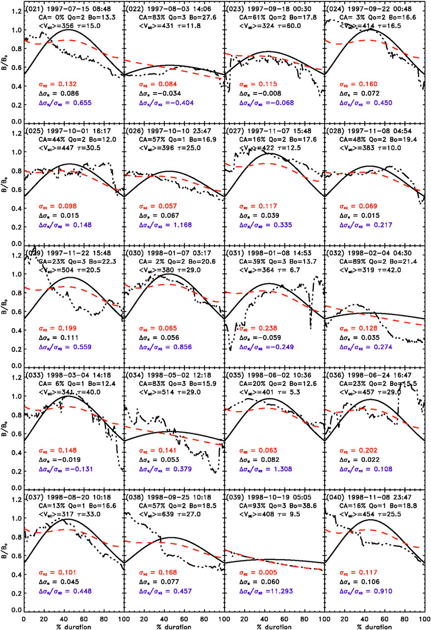
FIGURE 3. Example page (p. 2) of set of 11 pages (20 panels each) of the same quantities as shown in Figure 1, and in the same format, of Wind MCs from launch to July of 2015.
First, case #039 shows a value of ΔσN/σN2 of 11.29, which is unusually high (indicating a good result, even though Q0 = 3), because the value of σN2 = 0.005 is unusually small. We will not see many odd cases like this. Now consider good cases like #035 and #040, where ΔσN/σN2 is 1.31 (with Q0 = 2) and 0.91 (with Q0 = 1), respectively; both are well above 0.5. In both cases, we see the dramatic difference between the ability of the Quad scheme (dashed curve) to almost reproduce the observed values in the early part of the MC and the inability of the Bessel function (solid black curve) to do so in that part of the MC. Notice that #026 is similar to #035 in that they give similar values of ΔσN/σN2 (1.17 and 1.31, respectively) even though the first one has a somewhat long duration of 25.0 h and the second one has a rather short duration of only 5.3 h, and both of a quality that differs from Q0 = 3. Now we consider a very poor case, #022, that is, where ΔσN/σN2 is negative and rather large in the absolute value, where ΔσN/σN2 is −0.40 (with Q0 = 3). Case #033 is interesting in that the Quad scheme does well in the early part of the MC but not in the middle or latter regions, i.e. not as well as the Bessel field, so ΔσN/σN2 is negative, −0.13; notice that this is a very long duration MC of 40.0 h, and Q0 = 1. Those cases where the observed field is significantly lower in relative intensity than the Bessel function field, early in the MC, will usually produce the poorest results, such as in cases #022 and #031. This does not occur very frequently.
5 Conclusion and Discussion
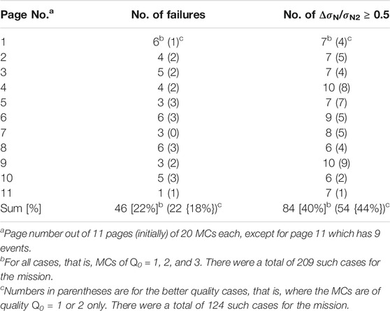
Here, we describe a new NASA Website (see Section 3) that provides normalized magnetic field (B/Bo) magnitude profiles within Wind MCs in terms of observations versus the basic-LJB model versus the Quad-modified model for 209 MCs that cover the period from launch (late 1994) to July of 2015. The model-modification is based on the studies of Lepping et al. [12] and Lepping et al. [10]. The basic force free MC parameter fitting model that is modified is that of LJB. The statistics of both the number of MC-modified failures and the number of (very good) cases where ΔσN/σN2 ≥ 0.5 given by this new website to this point (July 2021) is provided in Table 1.
For all cases (i.e., MCs of Q0 = 1, 2, and 3), Table 1 shows that the percentage of failures is 22%, and for the cases where Q0 = 1 and 2, only (values in parentheses) the percentage slightly improves to 18%. However, considering all cases, we find that 40% have ΔσN/σN2 ≥ 0.5, but the percentage slightly increases to 44% when the cases are restricted to Q0 = 1 and 2 only.
Figure 4 gives a histogram (called f (obs) and shown by a solid black curve) representing the frequency of occurrence of the observed ratio ΔσN/σN2 for the full Wind mission (i.e., from launch to July 2015), and for Q0 = 1, 2, and 3, and showing some key features, such as having a peak at about 0.5, a relatively small number of events greater than 1.0. It appears to be a slightly modified normal distribution. Since the histogram peaks near ΔσN/σN2 = 0.5, we choose it as a separator of “acceptable” from “very good” values of ΔσN/σN2. In fact, the curve f (obs) appears to be quite well fitted with a simple skewed Gaussian distribution (called f(Z) here):
where Z ≡ ΔσN/σN2, for c1 = 48, c2 = 0.35, and c3 = 0.55 (see [14]); the skewness factor is (1—c4Z), where c4 = 0.35. f(Z) is shown in Figure 4 as the red dashed curve. For a measure of how well this modified normal distribution fits the actual histogram, we define a σ as follows:
where i goes from 1 to 11, and therefore, N in this case is 11 (but recall that the total number of MCs employed in this analysis is 209). The value of σ = 4.0 is shown in the upper right-hand corner (first line in red) of Figure 4. For comparison, for the same set of coefficients, except with no skewness (i.e., c4´ = 0.0), we get a larger σ´ = 7.0 seen on the second line; this simple Gaussian is the black dotted curve in Figure 4. And for a set of coefficients of c1 = 45, c2 = 0.35, c3 = 0.55, and c4 = 0.0, we get an intermediate value for σ´´ = 6.0 (not shown in Figure 4); this is an attempt to lower the peak in the black dotted curve in the figure. The set of coefficients giving σ = 4.0, where only two-place accuracy is needed, is probably the best set possible, or very close to it. As new MCs are found in future Wind data, they will be added to this website, and, of course, they may alter the optimum f(Z) fit curve.
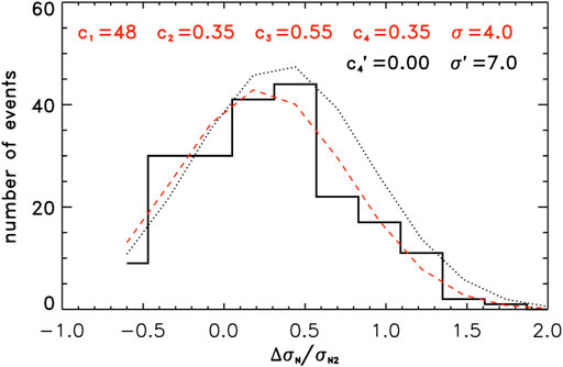
FIGURE 4. A histogram of frequency of occurrence of the observed ratio ΔσN/σN2 (black solid curve) with a superimposed skewed normal (Gaussian)-distribution, f(Z) (red dashed curve), where Z ≡ ΔσN/σN2; c1, c2, c3, and c4 are the coefficients shown in Eq. 1. The black dotted curve is for the same Gaussian (i.e., the same values of c1, c2, and c3), except now c4 is set equal to zero. σ gives a measure of how well the fit-curve approximates the observed histogram and is given by Eq. 2. The red coefficients hold for the red dashed skewed Gaussian and the black coefficients are for the simple Gaussian (second line at the top), where c1, c2, and c3 are the same in both cases. Note that both black and red curves are approximately Gaussian.
Finally, we discuss Figure 2 which is a plot of ΔσN/σN2 versus time for a family of Q0 (1, 2, and 3) showing almost the same average of ΔσN/σN2 (which goes from 0.43 to 0.48) regardless of the value of Q0, but with large scatter in each case. This means that there is a very poor correlation between ΔσN/σN2 and Q0. In other words, better values of ΔσN/σN2 should not necessarily be expected, just because the MCs are of better Quality (based on the LJB model). However, as Table 1 shows, the better Q0 is we might expect statistically slightly better results in both the success rate and in the degree of excellence, that is, in the percentage of cases where ΔσN/σN2 ≥ 0.5.
Concerning the issue of solar cycle dependence, solid and dotted lines of Figure 5A show yearly occurrence frequency of all MC events, NYearly and MC events with ΔσN/σN2 ≥ 0.5, and NΔσN/σN2≥0.5. The correlation coefficient between them is 0.94; that is, they correlate very well. Both NYearly and NΔσN/σN2≥0.5 vary with solar activity. Figure 5B shows clearly that there is no solar cycle dependence for normalized NΔσN/σN2≥0.5 with NYearly.
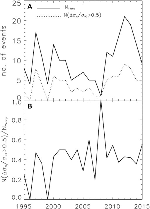
FIGURE 5. (A) Yearly occurrence frequency of all MC events, NYearly (solid-lines), and MC events with ΔσN/σN2 ≥ 0.5, NΔσN/σN2 ≥0.5 (dotted line). (B) Normalized yearly NΔσN/σN2≥0.5 with NYearly.
Speed is also an important input parameter for the LJB model. We separate 209 MCs into two groups: 1) ΔσN/σN2 < 0.5 and 2) ΔσN/σN2 ≥ 0.5. There are 123 MCs with ΔσN/σN2 < 0.5 and 86 MCs with ΔσN/σN2 ≥ 0.5. The average and median speed are 440 and 405 km/s, respectively, for group (1). The average and median speed are 433 and 408 km/s, respectively, for group (2). This implies that the Quad technique does not work better for the MC events with higher speed.
The Quad modification is derived from the difference in field magnitude between the actual field profiles and the fields derived from the LJB (Bessel function) model where many cases are considered, to develop quadratic correction functions. We have shown that in general, the LJB model with the Quad modification is expected to provide more accurate MC fitting, and it should be useful particularly for those studies where the spatial variation of the B-field magnitude across a MC is important, especially in comparison to the basic LJB model.
Data Availability Statement
The original contributions presented in the study are included in the article/Supplementary Material; further inquiries can be directed to the corresponding author.
Author Contributions
C-CW, RL, and DB contributed to conception and design of the study. C-CW organized the database. RL and C-CW performed the statistical analysis. RL wrote the first draft of the manuscript. RL, C-CW, and DB wrote sections of the manuscript. All authors contributed to manuscript revision, reading, and approved the submitted version.
Funding
This study was partially supported by the Chief of Naval Research (CCW), NASA 80HQTR19T0062 (CCW & RPL), 80HQTR18T0023, and 80HQTR20T0067 (CCW) grants.
Conflict of Interest
The authors declare that the research was conducted in the absence of any commercial or financial relationships that could be construed as a potential conflict of interest.
Publisher’s Note
All claims expressed in this article are solely those of the authors and do not necessarily represent those of their affiliated organizations, or those of the publisher, the editors, and the reviewers. Any product that may be evaluated in this article, or claim that may be made by its manufacturer, is not guaranteed or endorsed by the publisher.
Acknowledgments
We thank the Wind MFI and SWE teams for the care that they employ in producing the magnetic field and plasma data.
Supplementary Material
The Supplementary Material for this article can be found online at: https://www.frontiersin.org/articles/10.3389/fphy.2021.712599/full#supplementary-material
References
1. Burlaga L, Sittler E, Mariani F, Schwenn R Magnetic Loop Behind an Interplanetary Shock: Voyager, Helios, and IMP 8 Observations. J Geophys Res (1981) 86:6673–84. doi:10.1029/ja086ia08p06673
2. Burlaga LF Magnetic Clouds and Force-Free Fields with Constant Alpha. J Geophys Res (1988) 93:7217–24. doi:10.1029/ja093ia07p07217
4. Cane HV, Richardson IG Interplanetary Coronal Mass Ejections in the Near-Earth Solar Wind during 1996–2002. J Geophys Res (2003) 108:1156. doi:10.1029/2002JA009817
5. Jian L, Russell CT, Luhmann JG, Skoug RM Properties of Interplanetary Coronal Mass Ejections at One AU during 1995 – 2004. Solar Phys (2006) 239:393–436. doi:10.1007/s11207-006-0133-2
6. Chi Y, Shen C, Wang Y, Xu M, Ye P, Wang S, et al. Statistical Study of the Interplanetary Coronal Mass Ejections from 1995 to 2015. Sol Phys (2016) 291:2419–39. doi:10.1007/s11207-016-0971-5
7. Lepping RP, Berdichevsky DB, Wu C-C, Szabo A, Narock T, Mariani F, et al. A Summary of WIND Magnetic Clouds for Years 1995-2003: Model-Fitted Parameters, Associated Errors and Classifications. Ann Geophys (2006) 24:215–45. doi:10.5194/angeo-24-215-2006
8. Lepping RP, Wu C-C, Berdichevsky DB, Szabo A Magnetic Clouds At/near the 2007 - 2009 Solar Minimum: Frequency of Occurrence and Some Unusual Properties. Sol Phys (2011) 274:345–60. doi:10.1007/s11207-010-9646-9
9. Lepping RP, Wu C-C, Berdichevsky DB, Szabo A Wind Magnetic Clouds for 2010 - 2012: Model Parameter Fittings, Associated Shock Waves, and Comparisons to Earlier Periods. Sol Phys (2015) 290:2265–90. doi:10.1007/s11207-015-0755-3
10. Lepping RP, Wu C-C, Berdichevsky DB, Kay C Magnetic Field Magnitude Modification for a Force-free Magnetic Cloud Model. Solar Phys (2018) 293(19):162. doi:10.1007/s11207-018-1383-5
11. Lepping RP, Wu C-C, Berdichevsky DB, Szabo A Model Fitting of Wind Magnetic Clouds for the Period 2004 – 2006. Solar Phys (2020) 295:83. doi:10.1007/s11207-020-01630-2
12. Lepping RP, Berdichevsky DB, Wu C-C Average Magnetic Field Magnitude Profiles of Wind Magnetic Clouds as a Function of Closest Approach to the Clouds’ Axes and Comparison to Model. Solar Phys (2017) 292(2):27. doi:10.1007/s11207-016-1040-9
13. Lepping RP, Jones JA, Burlaga LF Magnetic Field Structure of Interplanetary Magnetic Clouds at 1 AU. J Geophys Res (1990) 95:11957. doi:10.1029/ja095ia08p11957
Keywords: magnetic cloud, force free model, magnetic field intensity, solar wind, Wind-MC
Citation: Wu C-C, Lepping RP and Berdichevsky DB (2021) Magnetic Field Intensity Modification to Force Free Model of Magnetic Clouds: Website of Wind Examples From Launch to July of 2015. Front. Phys. 9:712599. doi: 10.3389/fphy.2021.712599
Received: 20 May 2021; Accepted: 19 July 2021;
Published: 20 October 2021.
Edited by:
Hongqiang Song, Shandong University, ChinaReviewed by:
Miguel A. Hidalgo, University of Alcalá, SpainSimon Good, University of Helsinki, Finland
Yutian Chi, University of Science and Technology of China, China
Copyright © 2021 Wu, Lepping and Berdichevsky. This is an open-access article distributed under the terms of the Creative Commons Attribution License (CC BY). The use, distribution or reproduction in other forums is permitted, provided the original author(s) and the copyright owner(s) are credited and that the original publication in this journal is cited, in accordance with accepted academic practice. No use, distribution or reproduction is permitted which does not comply with these terms.
*Correspondence: Chin-Chun Wu, Y2hpbi1jaHVuLnd1QG5ybC5uYXZ5Lm1pbA==
 Chin-Chun Wu
 R. P. Lepping2,3