 Pengtao Zhang1*
 Jiwei Xu
95% of researchers rate our articles as excellent or good
Learn more about the work of our research integrity team to safeguard the quality of each article we publish.
Find out more
ORIGINAL RESEARCH article
Front. Phys. , 24 September 2021
Sec. Social Physics
Volume 9 - 2021 | https://doi.org/10.3389/fphy.2021.702064
In recent years, the global temperature is continuously rising and has the trend of accelerating. The frequent occurrence of extremely high temperatures and heat waves has caused widespread concern from all walks of life. How to fully understand the change law of temperature becomes very important. In view of the temperature change in Xi’an, this paper introduces a new method called visibility graph to establish the temperature network in Xi’an. On this basis, firstly, this paper studies the relationship between temperature fluctuation and network degree. We find that short-term fluctuations do not cause long-term effects. Then, through the study of network degree distribution, it is revealed that the temperature network conforms to the law of power-law distribution. In addition, this paper also completes the community detection of temperature network, and finds that some communities have fewer nodes (between June and August), which means that the correlation between summer temperature and other seasons in Xi’an is low, and it is easy to form extreme weather. To sum up, the research in this paper provides a new theoretical method and research ideas for mining and mastering the variation law of temperature in Xi’an.
During the past decades, our human society has experienced rapid development; while in modern industrial society, extreme weather-climate events seem to occur more frequently than ever before and the global warming has become a serious problem [1]. The climate change, especially the frequent occurrence of extreme climate events, is likely to affect our human society form different perspectives, such as, precipitation, crop growth and even daily habits which might incur enormous economic losses [2, 3]. At present, the continuous change of global temperature, especially climate warming, restricts the development of the regional economy and agriculture [4] , and has a great impact on the development of the social economy, which has attracted the attention of academic circles [5]. In addition, the greenhouse effect caused by the increase of greenhouse gases has produced a great threat to the lives of various organisms [7–9] It can be said that global warming will not only harm the economic development and social progress of the world, but also affect the living environment of humankind. In this context, this paper analyzes the characteristics of temperature change to fully understand and master the law of climate change. In this way, human beings can make scientific and rational use of climate resources to develop the economy and optimize the living environment.
In this manuscript, we present a complex network-based method in order to characterize the property of climate change of Xi’an for the past 10 years while the network is constructed through a visibility algorithm. Here, the highest temperature of a day is regarded as the temperature of that day. Along this line, characteristics of the obtained networks, such as the degree, degree distribution and community structure can be analyzed accordingly.
This manuscript is organized as follows: firstly, some related works are provided aiming to illustrate the state of art of this topic then, in the Model section, the proposed model is provided. Later, characteristics of the temperature data for Xi’an are presented and experiments are conducted with sufficient analyses. Finally, we conclude the manuscript.
In 1976, the World Meteorological Organization (WMO) first claimed that climate change can pose a serious threat to human society, people have paid more and more attention to climate change. Especially in recent years, global warming is becoming a popular issue of widespread concern to governments and scholars of various countries.
At present, the main research results on the evolution law of air temperature mainly focus on the change trend, change period, break point and asymmetry of temperature evolution. The study of Eastern D R et al. [10] shows that the daily temperature range in most parts of the world is decreasing continuously, mainly due to the difference between the change of daily maximum and minimum temperature. At the same time, they found that some circulation changes in the northern hemisphere seem to be related to the change of the daily temperature difference. Karl T R et al. [11] show that the average daily minimum temperature is on the rise. In addition, the decrease of daily temperature difference is approximately equal to the increase of average temperature, and the decrease part is related to the increase of cloud cover. In the study of the change cycle of temperature, on the one hand, we can use the ice core of Antarctica to obtain the temperature and atmospheric carbon dioxide changes in the past six glacier cycles [12], on the other hand, we can use the lower tropospheric channel of MSU satellite to obtain satellite remote sensing derived data set [13]. In terms of temperature evolution breakpoints, a variety of statistical methods are mainly used to analyze whether there is heterogeneity or mutation point in the meteorological data series, or to detect the mutation time [14]. The asymmetry of temperature is mainly to study the relationship between daily maximum temperature, minimum temperature and the temperature difference between day and night [15], to formulate appropriate strategies to deal with climate change.
There are three main research methods. The first method is applied forecasting. Human beings have been observing weather phenomena and climate change for a long time. On this basis, a large number of proverbs have been summed up and empirical analysis of weather has been done [16]. The second method is the numerical method. Based on numerical simulation, the continuous stochastic equation [17], thermal equation [18], kinematic equation and state equation [19] are used to fit atmospheric numerical value, to achieve the purpose of analyzing meteorology and temperature. The third method is model analysis [20–22]. This method uses probability and statistics theory to extract the temperature change law from the meteorological historical data, and it is also used to construct the statistical model. At present, the numerical method is the most used method with high accuracy. However, its calculation process is complex, and the initial value is sensitive. In addition, the atmospheric system is a complex nonlinear dynamic system, which makes the implementation of numerical prediction difficult.
With the penetration of complex network theory in various disciplines, it has become a new research method in the field of climate. By studying the topology of the network, we can analyze the characteristics of nodes and the whole system greatly. Therefore, this paper adopts a new method, visibility graph, to construct a network from time series, and it is used to establish the global and local temperature network of Xi’an. By observing the evolution characteristics of the network, we analyze and obtain the characteristics and laws of temperature fluctuation in Xi’an.
A practical system, such as social network, power system and aviation system, can usually be depicted as a network (graph)
In the network, degree represents the number of connections between one node and other nodes, and the distribution of degree of all nodes is called degree distribution. Degree distribution is very important for the research of real networks (such as the Internet, social networks, theoretical networks, etc.). The degree distribution of real networks has many characteristics, such as a long tail. The long tail characteristic means that the degree of most nodes in the network is small, and the degree of a few nodes is relatively large. In some networks, especially in real networks such as the Internet and social networks, the distribution of degree approximates the power-law distribution:
Where γ is a constant, and such networks are called scale-free networks [23].
Community structure is one of the most important characteristics of complex networks. Community detection is an effective method to analyze the properties of complex networks. Generally speaking, a community structure is a set of connected nodes. There are more connections between nodes in the set, but fewer connections between nodes in the set and nodes outside the collection. The purpose of community detection is to find the community structure in the network, to better study the topological structure of the network, mine the function of the network and reveal the law of the network and infer the evolution trend of the network.
This paper uses the Louvain algorithm [24] to explore the community structure of the temperature network in Xi’an. Louvain algorithm is a modular algorithm, and its modularity is defined as:
where
In addition, in the Louvain algorithm, modularity increment is defined, which represents the change of modularity when two regiments move:
where
In this paper, the existed VG [25–28] theory is adopted in order to convert the continuous temperature series of Xi’an into a complex network with the construction process being illustrated in Figure 1. For a time series
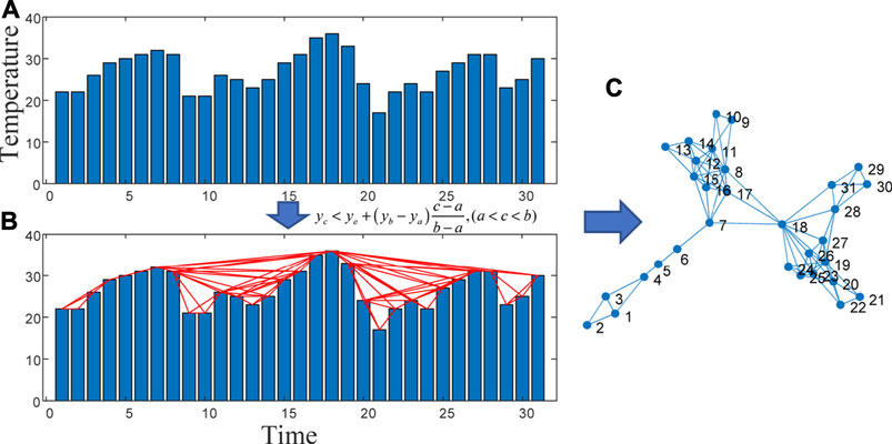
FIGURE 1. Illustration of the network construction process from climate data through VG theory. In (A,B), the abscissa is time (in days) and the ordinate is temperature (in°C). Where (A) is the original data, (B) is the network generated by Eq. 4, and (C) is the network structure presented as a graph.
It is found that the viewable network has the following properties: 1) There are no isolated nodes, and each node will at least be connected to its neighbors; 2) undirected, the generated network is undirected; 3) affine transformation invariance, and the affine transformation of the horizontal and vertical coordinates will not affect the network structure. The network generated from the visibility graph inherits some characteristics of time series, such as the transformation from periodic time series to regular network, from random time series to random network, and from fractal time series to scale-free network, etc.
This paper uses the temperature data of Xi’an from January 1, 2011 to October 31, 2020, with a total of 3,599 data (the temperature unit in this paper is in Centigrade) over the past 10 years. The data comes from China Weather Network, and the missing data is supplemented by other data sources such as China Meteorological administration. According to the visibility of the temperature data in Xi’an, we establish the temperature network of Xi’an, study the characteristics of the network by using the complex network theory, and reveal the internal mechanism of the temperature fluctuation in Xi’an.
In order to comprehensively analyze the characteristics of temperature change in Xi’an, we establish the global temperature network (all data from January 2011 to October 31, 2020) and local temperature network. We divide four 4 years time series windows, each of which is moved back 2 years to generate a new window, as shown in Figure 2. In adjacent time windows, there will be 2 years of the same data, each window has about 1,400 data.
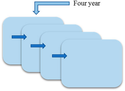
FIGURE 2. Time window.
In this paper, the purpose of selecting a time window is to obtain more properties of the network. For the temperature of Xi’an, a 4 year time window provides enough data for the construction of the network. By moving the time window, we can not only analyze the impact of the temperature in the last 2 years on the current 2 years’ temperature, but also analyze the impact of the current 2 years’ temperature on the next 2 years’ temperature, so as to realize the continuous transmission of information. The above window analysis method provides data for analyzing the evolution characteristics of the network indicators over time, which enables us to study the internal mechanism of temperature fluctuation in Xi’an.
It can be seen from Figure 3A that the temperature in Xi’an has a periodic variation law with the length of 1 year, although the variation law is not very clear. In contrast, the periodicity of network degree is less obvious. Generally speaking, if the temperature is high on a certain day, there will be a high network degree on that day. In the global network, the maximum degree of the network is 78 (the occurrence time is 2013/3/8 and 2017/7/21), and the corresponding time node temperature is 27 and 41 C respectively. It can be found that the node with a high degree is not a simple local maximum or a global maximum, but a node that has a great influence on the neighbor observation value. Before 2013/3, the temperature was in the continuous rising stage, and gradually turned clear from continuous snow rain and cloudy days. Before March 2013, the temperature was in the continuous rising stage, and gradually turned to clear from the continuous snow rain and cloudy days. Finally, the visibility degree of the node at 2013/3/8 was improved. On 2017/7/21, the highest temperature of the year reached 41 °C, which made the node have larger visibility. This law also appears in Figures 3B–E. In Figure 3B, the node with the largest degree also appears in 2013/3/8, and the degree is also 78. This means that short-term temperatures will not have a long-term effect. However, there are significant fluctuations at both ends of the time window, which are shown in the back end of Figure 3B, the front end of Figure 3E and the two ends of Figures 3C,D. This means that, as far as the temperature in Xi’an is concerned, short-term temperature fluctuation will only cause short-term impact.
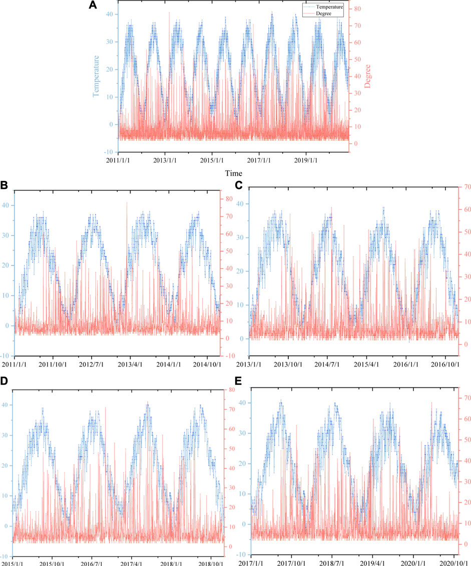
FIGURE 3. Temperature and network degree in Xi’an. (A) is a global network, (B–E) is a window network with a length of 4 years. In (A–E), the abscissa is time, the left ordinate is temperature, and the right ordinate is the degree of the network at the same time point.
In this section, we will analyze the degree distribution of the temperature network (as shown in Figure 4). When we study the degree of network, we find that the degree of some nodes is 2. This means that these nodes only have connections with adjacent nodes, and have no global impact. In order to better study the relationship between temperature, we combine the node set of degree 2 into the node set of degree 3. And to be more intuitive, we use the double logarithmic coordinate (base number is 10) for display, and use the power-law function
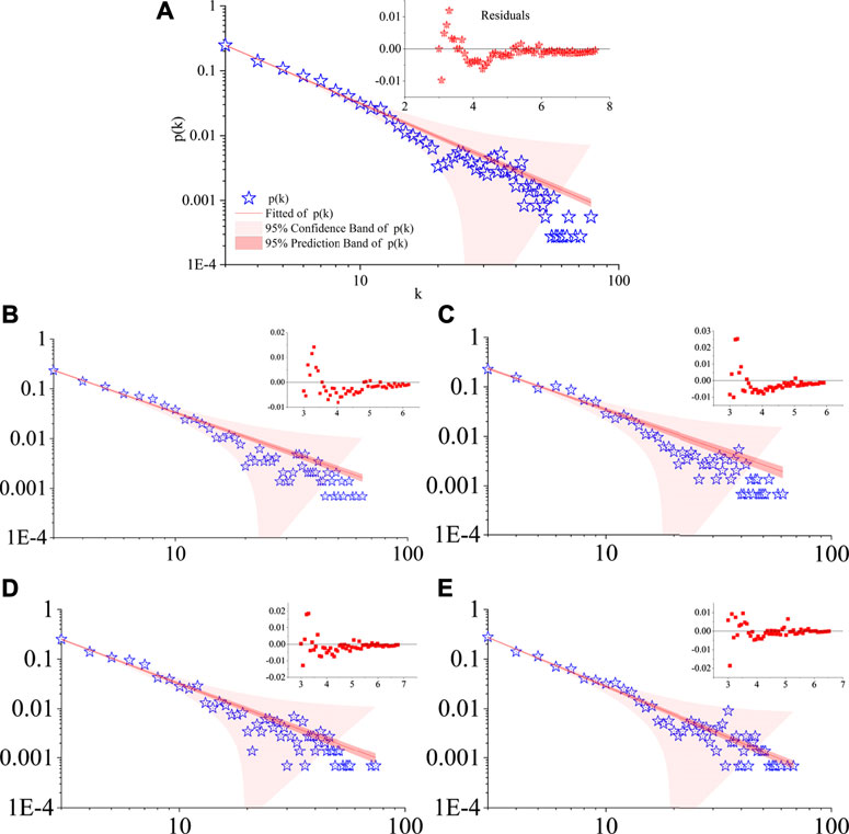
FIGURE 4. Degree distribution of networks. (A) is a global network, and (B–E) window network with a length of 4 years. In figures (A–E), the abscissa is the logarithm of degree with the base of 10, and the ordinate is the logarithm of frequency. The upper right corner of each pair is the fitting residual.
In Table 1, the degree fitting curves of the global temperature and each window in Xi’an are given, and the power-law index values
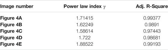
TABLE 1. Fitting results of Figures 4A–E.
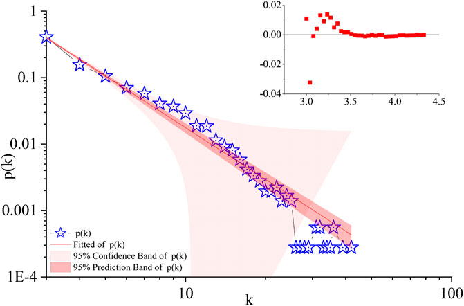
FIGURE 5. Distribution of temperature network degree in Xi’an randomly arranged.
Hurst index is often used to measure the long-term memory of time series. When H = 0.5, it indicates that time series can be described by random walk; When 0.5 < H < 1, it indicates that the time series has long-term memory; when 0 ≤ H < 0.5, it indicates that pink noise (anti persistence) is the mean recovery process. Therefore, we use rescaled range analysis (R/S) to calculate the Hurst index H of the time series, and the value of H is 0.4712. This shows that the temperature in Xi’an is negatively correlated with time, and there is no strong persistence. When the temperature in Xi’an rises in a certain period, it will decrease in the next period, that is, it has a strong mean regression characteristic, which is in line with the change characteristics of the annual temperature cycle. In other words, the temperature in Xi’an is highly elastic and is easily affected by factors such as wind, overcast, sunny, rain and snow.
For a given network, the nodes can be divided into different communities. In these communities, the nodes in the same community have a high degree of connectivity [29–33], while the connections between different communities are rare. The connection of the visibility graph is based on the visibility of the node, that is, nodes in the same community have great visibility. As far as experience is concerned, the correlation of temperature fluctuation in Xi’an is relatively high in a year cycle, and the temperature relationship in different years is relatively small. However, we still use the Louvain method to detect the community structure of global temperature in Xi’an. The results of community detection are shown in Figure 6, in which different communities are represented by different colors.
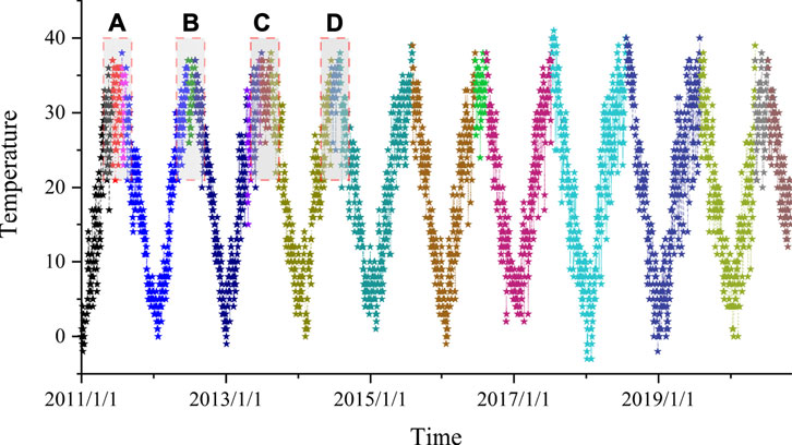
FIGURE 6. Community structure of global temperature network.
The community structure of the global temperature network in Xi’an is given in the network, there are 20 clusters in total, that is, the average annual temperature consists of two clusters. In this process, an interesting phenomenon is found: a community with fewer nodes will be formed from June to September every year, as shown in Figures 7A–D, which indicates that there is little relationship between the temperature during this period and the annual temperature, that is, the fluctuation of annual temperature will not affect the temperature in this period, and the temperature in this period will not have a significant impact on the annual temperature. This pattern appears six times in a decade. And it appears every time in the season with the highest temperature in Xi’an. Compared with other months, the climate in summer in Xi’an is more changeable. When it is sunny, it will appear the highest temperature of the year, and in rainy weather, the temperature will drop rapidly, showing a large fluctuation. There are 71 days between June 1, 2011 and August 10, 2011, and only 9 days are sunny. The time of 6 days is in the transition between sunny days and other weather. In contrast, there are 27 rainy days and 17 cloudy days. Under the current background of global warming, the temperature fluctuation between June and August in Xi’an provides necessary conditions for the occurrence of extreme weather, which leads to the problem that compared with the same period of previous years, Xi’an has more high-temperature days above 35°C, and the probability of periodic high-temperature heat waves, large-area summer drought and other extreme events is relatively high. There are three main reasons for extreme high temperature in Xi ‘an: geographical reasons, foehn effect and heat island effect. In terms of geographical location, Xi’an is located in the middle of the Guan Zhong Plain, with a warm temperate zone semi-humid continental monsoon climate. In summer, the sun shines directly on the northern hemisphere. Due to the low height of the sun and the long day time, the ground receives more solar radiation, which leads to a higher surface temperature. The second reason is the foehn [34]. In summer, the southeast monsoon prevails in most parts of China. When the southeast monsoon passes over the Qinling Mountains, the air stream will sink, causing the temperature in Xi’an to rise. The third reason is the heat island effect. Based on the quantitative analysis of anthropogenic heat emission of large cities in China, it is found that Xi ‘an belongs to the contributing area of strong heat island, next only to Shenzhen and Wuhan [35, 36].
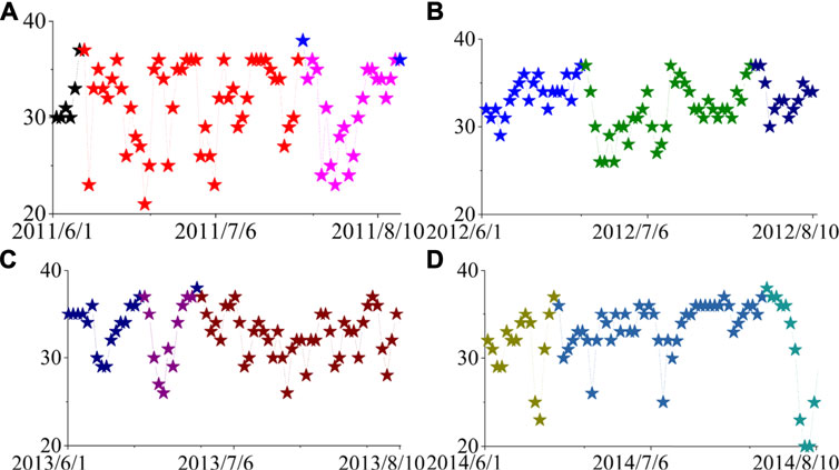
FIGURE 7. Local magnification of Figure 6.
Scientific observations since the beginning of this century have shown that the concentrations of various greenhouse gases in the atmosphere are increasing, and the average temperature of the earth will also increase greatly. In this context, the study of temperature change in Xi’an can provide references for the scientific development of agriculture, tourism, and daily travel. This paper introduces the visibility algorithm to convert the time series Xi’an temperature into a network, and analyzes the degree, degree distribution and community structure of the network. In general, the temperature network of Xi’an presents power-law distribution, and the power-law index ranges from 1.58 to 1.89 (the data also show power-law distribution after random arrangement). We calculate the Hurst index of random series, and the value of H is 0.4712, which means that the temperature in Xi’an is highly elastic and easily affected by wind, rain and snow. Through the research community, it is found that the temperature in Xi’an fluctuates greatly from June to August, and the weather is changeable during this period, which increases the probability of extreme weather. It can be said that our work provides a new research method and perspective for understanding and mastering the weather change law in Xi’an.
The original contributions presented in the study are included in the article/supplementary material, further inquiries can be directed to the corresponding authors.
PZ, and JX wrote sections of the manuscript. All authors contributed to manuscript revision, read, and approved the submitted version.
The authors declare that the research was conducted in the absence of any commercial or financial relationships that could be construed as a potential conflict of interest.
All claims expressed in this article are solely those of the authors and do not necessarily represent those of their affiliated organizations, or those of the publisher, the editors and the reviewers. Any product that may be evaluated in this article, or claim that may be made by its manufacturer, is not guaranteed or endorsed by the publisher.
1. Alkolibi FM. Possible Effects of Global Warming on Agriculture and Water Resources in Saudi Arabia: Impacts and Responses[J]. Climatic change (2002) 54(1-2):225–45. doi:10.1023/a:1015777403153
2. Osborne LF, Shaw BL, Mewes JJ, Salentiny DM. Continual Crop Development Profiling Using Dynamical Extended Range Weather Forecasting with Routine Remotely-Sensed Validation Imagery. U.S Patent 10,241,098[P] (2019).
3. Johnston AE, Poulton PR. The Importance of Long‐term Experiments in Agriculture: Their Management to Ensure Continued Crop Production and Soil Fertility; the Rothamsted Experience. Eur J Soil Sci (2018) 69(1):113–25. doi:10.1111/ejss.12521
4. Pretis F, Schwarz M, Tang K, Haustein K, Allen MR. Uncertain Impacts on Economic Growth when Stabilizing Global Temperatures at 1.5°C or 2°C Warming. Phil Trans R Soc A (2018) 376(2119):20160460. doi:10.1098/rsta.2016.0460
5. Kweku DW, Bismark O, Maxwell A, Desmond KA, Danso KB, Quachie AT, et al. Greenhouse Effect: Greenhouse Gases and Their Impact on Global Warming[J]. J Scientific Res Rep (2017) 1–9. doi:10.9734/JSRR/2017/39630
6. Calleja-Agius J, England K, Calleja N. The Effect of Global Warming on Mortality. Early Hum Dev (2020) 155(5):105222. doi:10.1016/j.earlhumdev.2020.105222
7. Liu B, Martre P, Ewert F, Porter JR, Challinor AJ, Müller C, et al. Global Wheat Production with 1.5 and 2.0°C above Pre‐industrial Warming. Glob Change Biol (2019) 25(4):1428–44. doi:10.1111/gcb.14542
8. Sun Q, Miao C, Hanel M, Borthwick AGL, Duan Q, Ji D, et al. Global Heat Stress on Health, Wildfires, and Agricultural Crops under Different Levels of Climate Warming. Environ Int (2019) 128:125–36. doi:10.1016/j.envint.2019.04.025
9. Baldos ULC, Hertel TW, Moore FC. Understanding the Spatial Distribution of Welfare Impacts of Global Warming on Agriculture and its Drivers. Am J Agric Econ (2019) 101(5):1455–72. doi:10.1093/ajae/aaz027
10. Easterling DR, Horton B, Jones PD, Peterson TC, Karl TR, Parker DE, et al. Maximum and Minimum Temperature Trends for the Globe. Science (1997) 277(5324):364–7. doi:10.1126/science.277.5324.364
11. Karl TR, Knight RW, Gallo KP, Peterson TC, Jones PD, Kukla G, et al. A New Perspective on Recent Global Warming: Asymmetric Trends of Daily Maximum and Minimum Temperature. Bull Amer Meteorol Soc (1993) 74(6):1007–23. doi:10.1175/1520-0477(1993)074<1007:anporg>2.0.co;2
12. Rohling EJ, Grant K, Bolshaw M, Roberts AP, Siddall M, Hemleben C, et al. Antarctic Temperature and Global Sea Level Closely Coupled over the Past Five Glacial Cycles. Nat Geosci (2009) 2(7):500–4. doi:10.1038/ngeo557
13. Herman BM, Brunke MA, Pielke RA, Christy JR, McNider RT. Satellite Global and Hemispheric Lower Tropospheric Temperature Annual Temperature Cycle. Remote Sensing (2010) 2(11):2561–70. doi:10.3390/rs2112561
14. García-Marín AP, Estévez J, Alcalá-Miras JA, Morbidelli R, Flammini A, Ayuso-Muñoz JL. Multifractal Analysis to Study Break Points in Temperature Data Sets. Chaos (2019) 29(9):093116. doi:10.1063/1.5096938
15. Zhuang Y, Zhang J. Diurnal Asymmetry in Future Temperature Changes over the Main Belt and Road Regions. Ecosystem Health and Sustainability (2020) 6(1):1749530. doi:10.1080/20964129.2020.1749530
16. Garteizgogeascoa M, García-del-Amo D, Reyes-García V. Using Proverbs to Study Local Perceptions of Climate Change: a Case Study in Sierra Nevada (Spain). Reg Environ Change (2020) 20(2):59. doi:10.1007/s10113-020-01646-1
17. Calif R, Schmitt FG. Modeling of Atmospheric Wind Speed Sequence Using a Lognormal Continuous Stochastic Equation. J Wind Eng Ind Aerodynamics (2012) 109:1–8. doi:10.1016/j.jweia.2012.06.002
18. Huang L, Liu J, He Y, Sun S, Chen J, Sun J, et al. Thermodynamics and Kinetics Parameters of Co-combustion between Sewage Sludge and Water Hyacinth in CO2/O2 Atmosphere as Biomass to Solid Biofuel. Bioresour Technology (2016) 218:631–42. doi:10.1016/j.biortech.2016.06.133
19. Thuburn J. Use of the Gibbs Thermodynamic Potential to Express the Equation of State in Atmospheric Models. Q.J.R Meteorol Soc (2017) 143(704):1185–96. doi:10.1002/qj.3020
20. Booz J, Yu W, Xu G, Griffithi D, Golmie N. A Deep Learning-Based Weather Forecast System for Data Volume and Recency Analysis[C]. 2019 International Conference on Computing, Networking and Communications (ICNC). 18-21 Feb. 2019. Honolulu, HI, USA. IEEE (2019). p. 697–701. doi:10.1109/ICCNC.2019.8685584
21. Fan J, Meng J, Ludescher J, Chen X, Ashkenazy Y, Kurths J, et al. Statistical Physics Approaches to the Complex Earth System. Phys Rep (2020) 896:1–84. doi:10.1016/j.physrep.2020.09.005
22. Dijkstra HA, Hernández-García E, Masoller C, Barreiro M. Networks in climate[M]. Cambridge University Press (2019). doi:10.1017/9781316275757
23. Barabási A-L, Bonabeau E. Scale-Free Networks. Sci Am (2003) 288(5):60–9. doi:10.1038/scientificamerican0503-60
24. Blondel VD, Guillaume J-L, Lambiotte R, Lefebvre E. Fast Unfolding of Communities in Large Networks. J Stat Mech (2008) 2008(10):P10008. doi:10.1088/1742-5468/2008/10/p10008
25. Lacasa L, Luque B, Ballesteros F, Luque J, Nuño JC. From Time Series to Complex Networks: The Visibility Graph. Pnas (2008) 105(13):4972–5. doi:10.1073/pnas.0709247105
26. Hu J, Xia C, Li H, Zhu P, Xiong W. Properties and Structural Analyses of USA's Regional Electricity Market: A Visibility Graph Network Approach. Appl Mathematics Comput (2020) 385:125434. doi:10.1016/j.amc.2020.125434
27. Zhang Y-J, Meng K, Gao T, Song Y-Q, Hu J, Ti E-P. Analysis of Attention on Venture Capital: A Method of Complex Network on Time Series. Int J Mod Phys B (2020) 34(29):2050273. doi:10.1142/s0217979220502732
28. Hu J, Li H-J, Gao J, Zhou Z, Xia C. Identifying Desirable Function Perturbations in Signaling Pathways through Stochastic Analysis. IEEE Access (2020) 8:15448–58. doi:10.1109/access.2020.2966229
29. Li HJ, Bu Z, Wang Z, CaoJ . Dynamical Clustering in Electronic Commerce Systems via Optimization and Leadership Expansion[J]. IEEE Trans Ind Inform (2019) 16(8):5327–34. doi:10.1109/TII.2019.2960835
30. Li HJ, Zhang J, Liu ZP, Chen L, Zhang XS. Identifying Overlapping Communities in Social Networks Using Multi-Scale Local Information Expansion[J]. The Eur Phys J B (2012) 85(6):1–9. doi:10.1140/epjb/e2012-30015-5
31. Li H-J, Wang L, Zhang Y, Perc M. Optimization of Identifiability for Efficient Community Detection. New J Phys (2020) 22(6):063035. doi:10.1088/1367-2630/ab8e5e
32. Li H-J, Wang Q, Liu S, Hu J. Exploring the Trust Management Mechanism in Self-Organizing Complex Network Based on Game Theory. Physica A: Stat Mech its Appl (2020) 542:123514. doi:10.1016/j.physa.2019.123514
33. Li HJ, Wang Z, Pei J, Cao J, Shi Y. Optimal Estimation of Low-Rank Factors via Feature Level Data Fusion of Multiplex Signal Systems[J]. IEEE Trans Knowledge Data Eng (2020) 13:33–9. doi:10.1109/TKDE.2020.3015914
34. Datta RT, Tedesco M, Fettweis X, Agosta C, Lhermitte S, Lenaerts JTM, et al. The Effect of Foehn‐Induced Surface Melt on Firn Evolution over the Northeast Antarctic Peninsula. Geophys Res Lett (2019) 46(7):3822–31. doi:10.1029/2018gl080845
35. Wang S, Hu D, Chen S, Yu C. A Partition Modeling for Anthropogenic Heat Flux Mapping in China. Remote Sensing (2019) 11(9):1132. doi:10.3390/rs11091132
Keywords: visibility graph, time series, community detection, complex network, temperature
Citation: Zhang P, Ning P, Cao R and Xu J (2021) Analysis of Climate Change Characteristics in Xi’an Based on the Visibility Graph. Front. Phys. 9:702064. doi: 10.3389/fphy.2021.702064
Received: 29 April 2021; Accepted: 23 August 2021;
Published: 24 September 2021.
Edited by:
Hui-Jia Li, Beijing University of Posts and Telecommunications (BUPT), ChinaReviewed by:
Jingfang Fan, Beijing Normal University, ChinaCopyright © 2021 Zhang, Ning, Cao and Xu. This is an open-access article distributed under the terms of the Creative Commons Attribution License (CC BY). The use, distribution or reproduction in other forums is permitted, provided the original author(s) and the copyright owner(s) are credited and that the original publication in this journal is cited, in accordance with accepted academic practice. No use, distribution or reproduction is permitted which does not comply with these terms.
*Correspondence: Pengtao Zhang, emhhbmdfZWR1MjAyMUAxNjMuY29t; Jiwei Xu, eHVAeHVwdC5lZHUuY24=
Disclaimer: All claims expressed in this article are solely those of the authors and do not necessarily represent those of their affiliated organizations, or those of the publisher, the editors and the reviewers. Any product that may be evaluated in this article or claim that may be made by its manufacturer is not guaranteed or endorsed by the publisher.
Research integrity at Frontiers
Learn more about the work of our research integrity team to safeguard the quality of each article we publish.