 Sebastian Littin
- 1Medical Physics, Department of Radiology, Faculty of Medicine, University Freiburg, Freiburg, Germany
- 2High Field MR Center, Center for Medical Physics and Biomedical Engineering, Medical University of Vienna, Lazarettgasse, Austria
The design of gradient coils is sometimes perceived as complex and counterintuitive. However, a current density is connected to a stream function in fact by a simple relation. Here we present an intuitive open source code collection to derive stream functions from current densities on simple surface geometries. Discrete thin wires, oriented orthogonally to the main magnetic field direction are used to describe a surface current density. An inverse problem is solved and stream functions are derived to find coil designs in the current and stream function domains. The flexibility of the design method is demonstrated by deriving gradient coil designs on several different surface topologies. This collection is primarily intended for teaching, as well as for demonstrating all gradient coil design steps with openly available software tools.
1 Introduction
Gradient coils are the key component to enable imaging using nuclear magnetic resonance (NMR). Spatially varying magnetic fields are switched in a time dependent manner to achieve spatial encoding of the NMR signals. Different approaches to gradient coil design have been proposed over the past decades to derive very sophisticated designs compared to initially implemented Maxwell and Golay type coils [1,2].
Most approaches to gradient coil design today are based on boundary element methods [3,4]. These approaches are based on representing the actual electrical current density by its stream function discretized on a surface mesh. Due to the counterintuitive approximation of a surface current density by equidistant iso-contour lines of the stream function the coil design problem is oftentimes perceived as complex. However, the relation between the current density and stream function is oftentimes perceived as complex. For educational purposes the level of complexity of the boundary element method can be reduced to understand and design simple gradient coils. The coil design problem can be derived intuitively with an intermediate step which represents the current density. In addition it can be simplified by reducing its dimensionality if the current carrying surface is oriented in parallel to the main magnetic field. This is done by neglecting currents which flow in parallel to B0 and therefore do not generate a Bz component relevant for encoding. Therefore we propose the most simple framework for coil design based on thin wires oriented orthogonally to the main magnetic field. This paper aims at providing an intuitive access to gradient coil design. Additionally, Stream functions are derived from an intermediate representation of current densities and by a direct solution. The straight-forward, yet powerful approach presented here is suitable for simple, regular surface geometries such as cylinders or planes.
Most coil designs are derived by deploying commercially available closed source software, e.g. [5,6]. To the knowledge of the authors there is no code openly available which includes the surface mesh definition for gradient coil design, as well. One repository available on GitHub by Bringout et al. [7]. needs a predefined triangular surface mesh. Here, the mesh definition is included within the code that accompanies this paper and the complete sources are available on GitHub.
2 Theory and Methods
All scripts to demonstrate this method were designed to run with GNU Octave and MatLab (The Mathworks, Nattick, MA, United States). Images in this manuscript were plotted with GNU Octave on a laptop computer.
Gradient coils for spatial encoding are usually operated with frequencies below 10kHz, therefore the coil design may be treated as a magneto-static problem. The relation between the magnetic field of the gradient coil, B(r), and a free current density, J(r), is given by Ampere’s law:
where μ0 is the permeability of free space.
Conventional magnetic resonance imaging (MRI) usually deploys a main magnetic field which is highly uniform, unidirectional and very strong to achieve a sufficient spin polarization. Due to its historic origin from NMR, direction of the main field B0 is by convention chosen along the z-axis. The local Larmor precession frequency only depends on the absolute value of the superposition of the main magnetic field and the field induced by the gradient coil. A Taylor expansion of this magnitude of the superposition field yields
where
Thin-Wire Approximation
For simple, regular surface geometries such as planar or cylindrical, a current density, J(r), may be approximated by discrete thin wire segments. As only Bz is considered relevant for spatial encoding and due to the curl operation as in Eq. 1 between the current and the generated magnetic field, the orientation of each current carrying element, m, is chosen to be orthogonal to the z-axis. Wires running parallel to B0 produce no Bz component and can be used in this model to feed the orthogonal current segments. All feeding wires are allowed to overlap in space, as wire thickness is ignored in the basic thin-wire approximation.
Each orthogonal thin-wire segment m with a current Im contributes to each target point n, which results in a spatially dependent magnetic field Bz,n, at point n, depicted in Figure 1A. The relation between the current in each thin-wire segment and the field of each point in space is described by the Biot-Savart law:
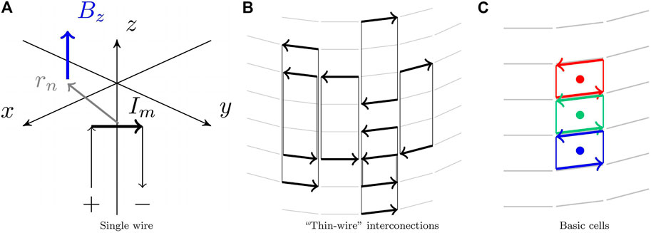
FIGURE 1. (A) One current carrying element which hosts a current Im generates a magnetic field component Bz at position rn. Multiple discrete thin wires which are oriented orthogonal to the direction of the main magnetic field, z, may be used to approximate a current density, J, on a regular surface. (B) A coil design may be realized with closed loops if there is a return path for each current flowing along z. (C) A basic rectangular cell of a boundary element is defined by combining two neighboring thin-wire elements with opposite current directions. Each color depicts one basic cell. If only Bz is considered this cell is composed of two parallel wires.
Combining these relations defines the sensitivity matrix Snm. By representing the currents in each thin wire segment as a vector, Im, and extracting only the Bz component of the field vector, simple algebraic expressions become possible. The resulting gradient field is defined by the column vector, Bz,n, according to
A corresponding current distribution for a given target field
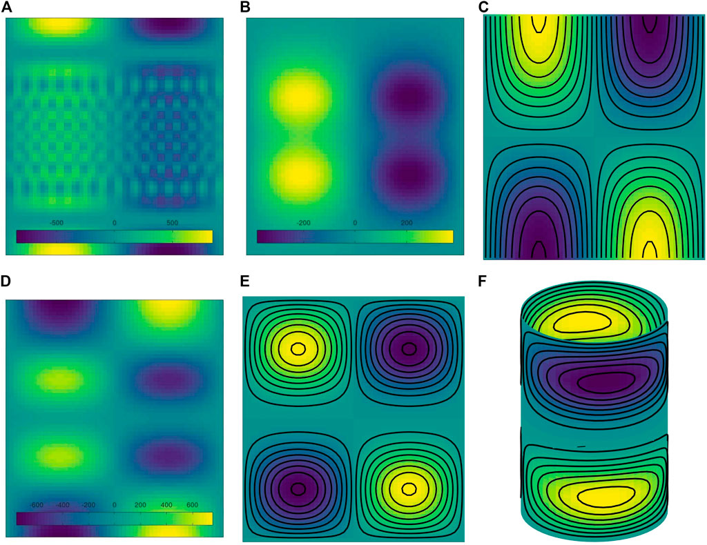
FIGURE 2. Different steps to illustrate gradient coil design based on a surface current density. Scales are in [A]. (A) An un-regularized current density results in high opposing currents and is therefore very inefficient. (B) Regularization penalizes opposing currents. (C) Integration along the z yields the stream function. However, the discrete wire paths which are given by streamlines are not realizable by closed loops. (D) An additional constraint is added to ensure that the sum of currents along z equals zero. (E) The corresponding wire paths are now realizable as closed loops. (F) A 3D-rendering may be plotted by the supplied code.
Power Optimization
A Tikhonov regularization may be used to find solutions with smaller norms, which penalizes high opposing currents according to the following minimization problem
Here,
The identity matrix in the Tikhonov regularization penalizes the sum of squares of the currents in each of the elements. This is proportional to the power dissipated by all elements and therefore acts to limit the total required electrical power. From a physics point of view the coefficient λ is related to the resistance of the wire segments. An appropriate choice of the weighting factor is balancing efficiency against accuracy of the resulting field. This free design parameter has to be chosen by the coil designer. Different approaches, e.g. the L-curve method [8] may be used to choose practical values. An exemplary regularized current distribution is shown in Figure 2B.
The Stream Function Representation and Discretization
Discrete wire layouts of gradient coil designs are usually derived from a stream function representation of surface currents. The stream function is then used to plot equidistant iso-contours, so called streamlines, representing trajectories of equally spaced steady flow of current. The number of streamlines is chosen according to engineering constraints, e.g. wire thickness, minimum wire spacing or maximum inductance.
The stream function is related to the current density by its integral. An integration of the previously regularized current density is depicted in Figure 2C. In matrix form, the integration may be directly acquired from the current density by calculating the cumulative sum along the z-direction according to
Here, it should be noted that the depicted discrete coil layout may not be realized by closed loops, leading to a gradient coil requiring many current terminals on each side. The example shown in Figure 2C would require current terminals and sinks of twice the number of iso-contours on each side, which is impractical.
Realizing Closed Loops
As depicted in Figure 2C, even the regularized current distribution may not be realizable in a straight-forward manner due to a high number of feeding ports. An additional constraint, enforcing the sum of currents along the z-axis to be zero along the surface boundaries, ensures for a design with closed loops. This constraint is given by
In this equation the index m is replaced by two indices, corresponding to the position of represented segments in the 2D matrix. Effectively, this is equivalent to Kirchhoff’s current law, which states the principle of the electric charge conservation. If this condition is fulfilled, for each current flowing along the direction orthogonal to z there is an opposing current, or currents with the same ij coordinate, present elsewhere along the z axis. Closed loops, including their feeding wires running in parallel to B0 needed to fulfill Eq. 8 are sketched in Figure 1B. Such interconnections along z might even be realized without altering the resulting target field Bz. On continuous surfaces of simple topologies this ensures a design which is realizable with closed current loops on this surface. In the practical implementation Eq. 8 can be converted to a matrix form and appended to Eq. 5 before solving the regularization problem.
Closed loop iso-contours derived from the stream function requires some manual interaction to get realizable gradient coil design, which can be manufactured by a single wire. Manual addition of connections between neighboring iso-contour lines transforms each quadrant into a spiral. Connections are usually chosen along the z-direction while return paths are positioned on top to mitigate effects from the introduced changes [9]. An automated process to interconnect multiple groups of streamlines has been proposed recently [10]. However, such an automatic approach is beyond the scope of this work.
Additional constraints may be added to enforce further design requirements. Exemplary mentioned here is the balance of force or torque which may be expressed by simple matrix operations, as well. Assuming thin wires which host currents In orthogonal to a strong and unidirectional main magnetic field Bz the force on each discrete element, n, is given by
To account for field inhomogeneities, the main magnetic field B needs to be defined at each wire location. Accordingly, the excess torque may now be calculated by summation over all moments from force F at position r. The resulting term
may be added and minimized during the optimization. A regularization parameter has to be added for an adequate weighting of the constraints. Balancing multiple regularization parameters is the art of coil design and usually requires a comparison of multiple designs within a reasonable parameter space [11].
From Current Distributions to Stream Functions
The thin-wire approximation provides an already powerful approach to find realizable gradient coil designs. However, the coil layout is not directly derived, but requires and intermediate step in the current domain.
For calculating stream functions, the boundary element method is usually deployed. Most methods are based on triangular meshes, each triangle describing one boundary element. However, finite element methods (FEMs) in general are not limited to triangular meshes. Boundary elements with a rectangular mesh may be used, as well (e.g. [12,13]). Considering only the z-component of the magnetic field, a simplified rectangular element may be derived from two neighboring thin wires, as used in the thin-wire approach. Since connecting paths along the z-axis do not contribute to Bz, they may be neglected. A basic cell from wire elements is sketched in Figure 1C.
Corresponding to the sensitivity matrix S (Eq. 4) a similar sensitivity matrix in the stream function domain Sstream may be derived. Size of the original sensitivity matrix S is given by the number of target points, n, the number of circumferential segments, mc, and number of segments along z, mz,
In analogy to the inverse problem stated in Eq. 5 a corresponding current value may be calculated. For regularizing this equation an effective current has to be used which consists of the combination from currents of two neighboring cells at the same location which can be achieved by an appropriate modification of the matrix Γ.
As previously shown, closed loops were enforced in the current domain by a constraint which was defined in a global manner (see Eq. 8). Due to the definition of the stream-function as spatial difference between two neighboring current carrying elements the same constraint does not lead to a meaningful result. Therefore closed loops have to be enforced using a different strategy. The approach chosen here was to demand the peripheral elements to carry zero current. This requires the addition of further terms to the inverse problem. Same currents of all outer elements, in this case zero, ensures closed stream lines. In analogy to the closed loops, further constraints may be added similarly. As stated above, this may include balance of force and torque, maximum current density or others.
The basic idea of the coil design method is demonstrated using the dimensions of a cylindrical whole-body gradient setup with a radius of 0.4 [m], a length of 1.2 [m], a mesh density of 56 angular by 61 longitudinal elements. A y-gradient with a 1 [mT/m] spherical target field with a radius of 0.2 [m] was chosen.
Besides a simple cylinder other geometries were simulated to demonstrate the variability of the method. This includes a shielded setup which consists of two independent cylindrical surfaces with radii of 0.4 [m] and 0.5 [m] and a length of 1.2 [m]. A thin-wire mesh of 48 angular by 61 longitudinal elements was chosen on each cylinder along with a spherical target with a radius of 0.15 [m].
A biplanar coil setup with two flat surfaces of 0.6 [m] × 0.6 [m] separated by 0.4 [m] with a mesh of 61 × 61 elements was used to demonstrate the feasibility of flat surfaces. The target region was chosen to be spherical with a radius of 0.15 [m].
An additional level of complexity is added for split gradient coils e.g. for multi-modality or combined MR-Linac systems [14,15]. Such coils in a shielded arrangement consist of four independent current carrying surfaces. Dimensions of the cylindrical shielded coil were used as a basis to simulate such a setup with radii of 0.4 [m] and 0.5 [m], a length of 0.6 [m] and a separation along z of 0.2 [m]. A thin-wire mesh of 48 angular by 61 longitudinal elements was chosen on each cylinder along with a spherical target with a radius of 0.15 [m]. Plots of each surface mesh are included in the code supplied with this paper.
The strength for each target field was set to 1 [mT/m] and the number of iso-contours was chosen to allow for a good visualization for plotting. It should be noted that the actual number of iso-contours is usually chosen based on constraints given by the overall system design. For larger coils the choice is a trade-off between efficiency and possible switching speed which is limited by the available maximum current and voltage. For smaller coils the number of iso-contours is mostly limited by the available space which is needed for a finite wire thickness.
3 Results
To demonstrate the versatility of the proposed method, stream functions based on discrete current distributions have been calculated for multiple different numbers of independent current carrying surfaces and different coil geometries. A gradient coil design on a single surface is given by the cylindrical design shown in Figure 2. The original target field along with the deviation of the resulting field is depicted in Figure 3. The regularization chosen here results in a deviation of about ±6%. This deviation may be controlled by the relation between the regularization and the chosen dimensions.
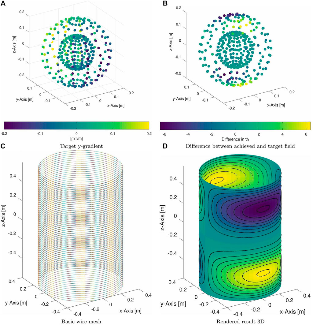
FIGURE 3. (A) A spherical y-gradient target with 1 [mT/m] was used for the cylindrical coil design. (B) The difference between target and generated field is depicted. (C) The mesh for the optimization consists of single individual wires which are oriented orthogonal to the main field direction. (D) 3D-rendering with dimensions of the resulting cylindrical whole-body gradient design.
Cylindrical shielded gradient coils are usually used in high-field MRI scanners to suppress eddy currents in the cryostat [16–18]. Therefore, a second target region is defined on a cylindrical surface at the position of the cold radiation shield. A wire mesh along with the main and shield target is shown in Figure 4. Compared to the main layer, the shield exhibits opposite polarity which corresponds to opposite direction of currents.
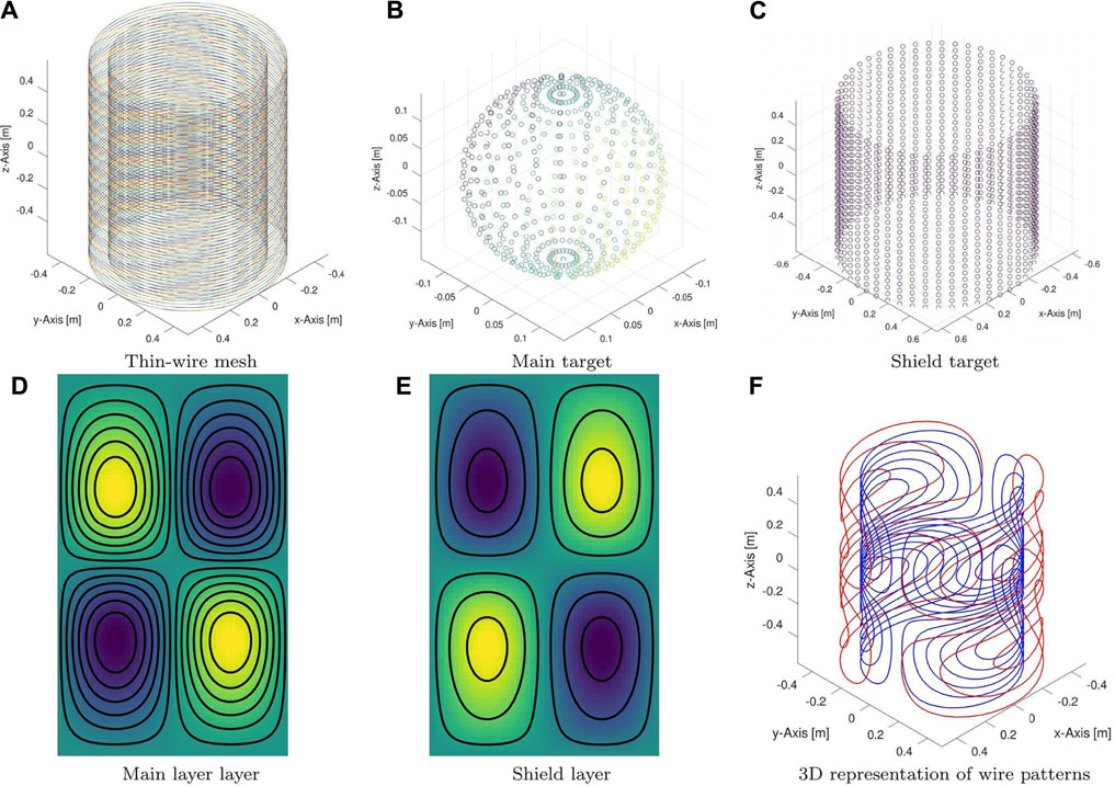
FIGURE 4. (A) The design of a shielded gradient coil hosts currents on two independent surfaces. In such a design the goal is to achieve a target field in center (B), while suppressing fields outside the coil. (C) The magnetic field on an additional cylindrical target surface, representing the cryostat, was set to zero. Depicted are (D) the main layer, (E) the shielding layer and (F) a combined representation of the resulting coil design.
A biplanar set of coils deploys two independent current carrying surfaces and is depicted in Figure 5. One should keep in mind that most biplanar setups in the literature are designed for a main magnetic field which is oriented along the vertical axis. However, this is not the case in the example shown here.
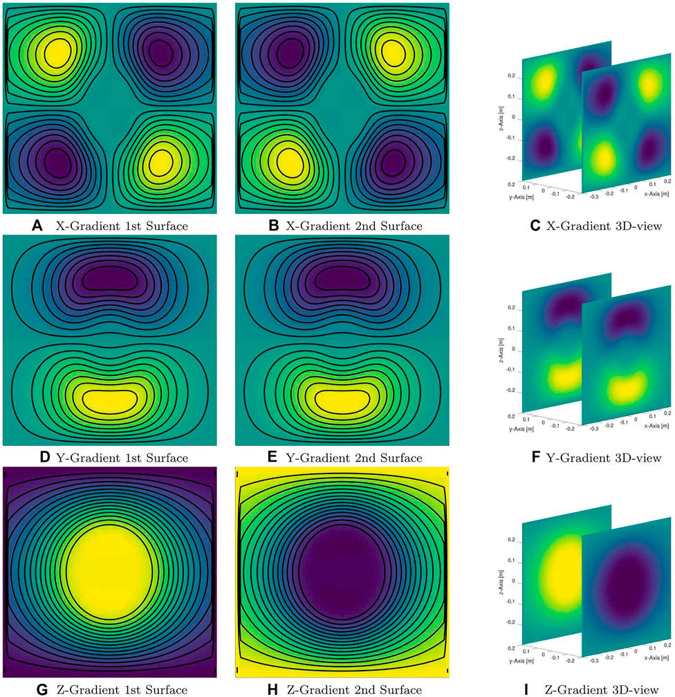
FIGURE 5. Bi-planar design to demonstrate the feasibility of using flat surface geometries. Direction of the main magnetic field is along the z-axis. Both surfaces (first and second row) along with a 3D visualization are shown for three different gradient fields. Currents on all edges of both surfaces had to be forced to zero for achieving closed loops.
An additional level of complexity is added in the design of split coils e.g. for multi-modality or combined MR-Linac systems [14,15]. Such coils in a shielded arrangement consist of four independent current carrying surfaces. Resulting wire layouts are shown in Figure 6. Same dimensions as for the previous shielded design and a gap of 0.2 m was chosen.
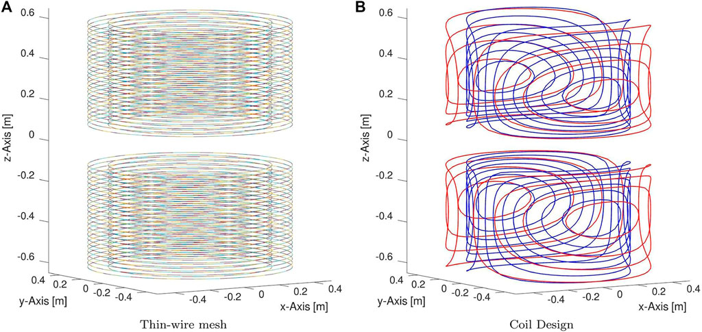
FIGURE 6. A shielded split coil design with four independent current carrying surfaces. Depicted are (A) the thin-wire mesh and (B) the resulting wire layout. Such designs are usually deployed in systems which combine linear accelerators for cancer treatment with MRI for imaging.
One of the main results is the code which was used to generate the rectangular thin-wire mesh and all designs within this manuscript. The full code is available as supporting material and under1.
4 Discussion
One of the main motivations for this work is the educational aspect, introducing gradient coil design in a straight-forward, intuitive and easy to understand way. To do so, we approach the gradient coil design from a current-density perspective. If the magnitude of the encoding field is much smaller than the main field strength a simplified representation becomes possible by considering the z-component of the magnetic field, only. Hence one field component instead of all three has to be calculated while significantly reducing the computational effort. Versatility of the proposed method is demonstrated by coil designs on flat and cylindrical surfaces. Coil designs on multiple independent current carrying surfaces are demonstrated by a shielded and a split shielded design.
The coil design methods shown are closely related to previously shown boundary element approaches, e.g. [3,4] which have been maximally reduced. Due to the reduction to Bz only, the optimization may not be usable directly for all magnet types. For classical and superconducting electromagnets the current carrying surface(s) are usually orthogonal to the main magnetic field, regardless of field strength. MRI systems based on rare Earth magnets are usually orientated such, that the current carrying surfaces of the gradient coils are not perpendicular to the direction of the main magnetic field. This includes u-shaped and Hallbach array type magnets [19–22] and others. However, the reduced form presented here may be easily adapted by adding longitudinal thin-wires to consider all field components, including Bxy, and closing the boundary element loops. Such a possible addition comes with an increased computational effort.
Due to the simplification using only wires orthogonal to the z-axis, the current method is limited to regular surface geometries. Methods for arbitrary surfaces have been shown e.g. in [5,23]. It should be noted that for manufacturing reasons most gradient coils are realized in fact on simple surfaces. However, with new manufacturing techniques based on 3D printed materials, such as shown in [24] other shapes might be used more often in the future. For such cases a full description of all components of the current density is also possible. For instance in the literature on the FEM methodology, approaches to shear and deform rectangular elements are usually covered, e.g. [12,13]. In the context of gradient coil design non-triangular mesh elements have been used, as well [25,26].
Minimum wire distance is one of the engineering constraints which has to be considered during the design. This has not been considered in the designs presented here and the associated problems are most apparent in the bi-planar designs in Figure 5. One approach is to choose the number of coil turns according to spatial constraints. More sophisticated approaches constrain the gradient of the stream function, the current density, using a minimax design or a p-norm [6,27]. Alternatively, an explicit constraint could be relatively trivially added directly to the thin-wire solver.
As a further step the iso-contour lines of the stream function have to be interconnected. A automatized interconnection algorithm has been demonstrated recently [10]. We hope that a combination of the intuitive approach to coil design shown here with an easy to use interconnection algorithm lowers the boundary for making experimental gradient coils.
A further goal of this publication was to make gradient coil design code which covers main aspects of the coil design problem, including surface mesh definition, available to the public. In addition to the supplemented materials, the code is available on GitHub under1. We hope that additional adaptations of the code are available in the future, including extensions to arbitrary orientations of the main magnetic field, e.g. for systems based on Halbach type magnets.
Data Availability Statement
The datasets presented in this study can be found in the Supplementary Material and on github: https://github.com/Sebastian-MR/ThinWire_MRIGradientCoilDesign.
Author Contributions
SL: Wrote code and manuscript FJ: Support with Code gradient design questions PA: Support with Code gradient design questions MZ: Initial code idea, supervision and guidance.
Funding
The article processing charge was funded by the Baden-Wuerttemberg Ministry of Science, Research and Art and the University of Freiburg in the funding program Open Access Publishing.
Conflict of Interest
The authors declare that the research was conducted in the absence of any commercial or financial relationships that could be construed as a potential conflict of interest.
Publisher’s Note
All claims expressed in this article are solely those of the authors and do not necessarily represent those of their affiliated organizations, or those of the publisher, the editors and the reviewers. Any product that may be evaluated in this article, or claim that may be made by its manufacturer, is not guaranteed or endorsed by the publisher.
Supplementary Material
The Supplementary Material for this article can be found online at: https://www.frontiersin.org/articles/10.3389/fphy.2021.699468/full#supplementary-material
Abbreviations
FEM, finite element method; MRI, magnetic resonance imaging; NMR, nuclear magnetic resonance.
Footnotes
1https://github.com/Sebastian-MR/ThinWire_MRIGradientCoilDesign
References
1. Turner R. Gradient Coil Design: A Review of Methods. Magn Reson Imaging (1993) 11:903–20. doi:10.1016/0730-725X(93)90209-V
2. Hidalgo-Tobon SS. Theory of Gradient Coil Design Methods for Magnetic Resonance Imaging. Concepts Magn Reson (2010) 36A:223–42. doi:10.1002/cmr.a.20163
3. Lemdiasov RA, Ludwig R. A Stream Function Method for Gradient Coil Design. Concepts Magn Reson (2005) 26B:67–80. doi:10.1002/cmr.b.20040
4. Poole M, Bowtell R. Novel Gradient Coils Designed Using a Boundary Element Method. Concepts Magn Reson (2007) 31B:162–75. doi:10.1002/cmr.b.20091
5. Handler WB, Harris CT, Scholl TJ, Parker DL, Goodrich KC, Dalrymple B, et al. New Head Gradient Coil Design and Construction Techniques. J Magn Reson Imaging (2014) 39:1088–95. doi:10.1002/jmri.24254
6. Jia F, Littin S, Layton KJ, Kroboth S, Yu H, Zaitsev M. Design of a Shielded Coil Element of a Matrix Gradient Coil. J Magn Reson (2017) 281:217–28. doi:10.1016/j.jmr.2017.06.006
7. Bringout G, Buzug TM. Coil Design for Magnetic Particle Imaging: Application for a Preclinical Scanner. IEEE Trans Magn (2015) 51:1–8. doi:10.1109/tmag.2014.2344917
8. Hansen PC The L-Curve and its Use in the Numerical Treatment of Inverse Problems In P. Johnston, editor Computational Inverse Problems in Electrocardiology Advances in Computational Bioengineering. Ashurst, UK: WIT Press (2000). p. 119–142.
9. Peeren GN. Stream Function Approach for Determining Optimal Surface Currents. J Comput Phys (2003) 191:305–21. doi:10.1016/s0021-9991(03)00320-6
10. Jia F, Littin S, Zaitsev M. Routing Algorithm for the Interconnection of Closed Wire Loops for Mr Gradient and Mr Shim Coils. Proceedings of the 2020 ISMRM and SMRT Virtual Conference and Exhibition (2020), 4070.
11. Cobos Sanchez C, Fernandez Pantoja M, Poole M, Rubio Bretones A. Gradient-coil Design: A Multi-Objective Problem. Conference Name: IEEE Transactions on Magnetics. IEEE Trans Magn (2012) 48:1967–75. doi:10.1109/TMAG.2011.2179943
13. Brenner SC, Scott LR. The Mathematical Theory of Finite Element Methods, 15. New York, NY: Springer (2008). doi:10.1007/978-0-387-75934-0
14. Poole M, Bowtell R, Green D, Pittard S, Lucas A, Hawkes R, et al. Split Gradient Coils for Simultaneous Pet-Mri. Magn Reson Med (2009) 62:1106–11. doi:10.1002/mrm.22143
15. Tang F, Freschi F, Sanchez Lopez H, Repetto M, Liu F, Crozier S. Intra-coil Interactions in Split Gradient Coils in a Hybrid MRI-LINAC System. J Magn Reson (2016) 265:52–8. doi:10.1016/j.jmr.2016.01.013
16. Mansfield P, Chapman B. Active Magnetic Screening of Coils for Static and Time-dependent Magnetic Field Generation in NMR Imaging. J Phys E: Sci Instrum (1986) 19:540–5. doi:10.1088/0022-3735/19/7/008
17. Roemer PB, Hickey JS. Self-shielded Gradient Coils for Nuclear Magnetic Resonance Imaging. Magn Reson Imaging (1986) 1986:1038–94. doi:10.1002/mrmp.22419860310
18. Bowtell R, Mansfield P. Gradient Coil Design Using Active Magnetic Screening. Magn Reson Med (1991) 17:15–21. doi:10.1002/mrm.1910170105
19. Halbach K. Strong Rare Earth Cobalt Quadrupoles. IEEE Trans Nucl Sci (1979) 26:3882–4. doi:10.1109/tns.1979.4330638
20. Halbach K. Design of Permanent Multipole Magnets with Oriented Rare Earth Cobalt Material. Nucl Instr Methods (1980) 169:1–10. doi:10.1016/0029-554X(80)90094-4
21. Raich H, Blümler P. Design and Construction of a Dipolar Halbach Array with a Homogeneous Field from Identical Bar Magnets: Nmr Mandhalas. Concepts Magn Reson (2004) 23B:16–25. doi:10.1002/cmr.b.20018
22. Cooley CZ, Haskell MW, Cauley SF, Sappo C, Lapierre CD, Ha CG, et al. Design of Sparse Halbach Magnet Arrays for Portable Mri Using a Genetic Algorithm. IEEE Trans Magn (2018) 54:1–12. doi:10.1109/tmag.2017.2751001
23. Lemdiasov RA, Ludwig R. A Stream Function Method for Gradient Coil Design. Concepts Magn Reson (2005) 26B:67–80. doi:10.1002/cmr.b.20040
24. Littin S, Jia F, Layton KJ, Kroboth S, Yu H, Hennig J, et al. Development and Implementation of an 84-channel Matrix Gradient Coil. Magn Reson Med (2018) 79:1181–91. doi:10.1002/mrm.26700
25. Zhu M, Xia L, Liu F, Zhu J, Kang L, Crozier S. A Finite Difference Method for the Design of Gradient Coils in MRI-An Initial Framework. IEEE Trans Biomed Eng (2012) 59:2412–21. doi:10.1109/TBME.2012.2188290
26. Kang L, Xia L, Wang Q, Wang Y, Tang F, Liu F. A Volumetric Finite-Difference Method for the Design of Three-Dimensional, Arbitrary-Structured Mri Gradient Coil. Rev Scientific Instr (2021) 92:034712. doi:10.1063/5.0035118
Keywords: magnetic resonance imaging, gradient coil design, MRI hardware, boundary element method, stream function, open source
Citation: Littin S, Jia F, Amrein P and Zaitsev M (2021) Methods: Of Stream Functions and Thin Wires: An Intuitive Approach to Gradient Coil Design. Front. Phys. 9:699468. doi: 10.3389/fphy.2021.699468
Received: 23 April 2021; Accepted: 31 August 2021;
Published: 28 September 2021.
Edited by:
Simone Angela S. Winkler, Cornell University, United StatesReviewed by:
Isabelle Saniour, Weill Cornell Medicine, United StatesFeng Liu, The University of Queensland, Australia
Copyright © 2021 Littin, Jia, Amrein and Zaitsev. This is an open-access article distributed under the terms of the Creative Commons Attribution License (CC BY). The use, distribution or reproduction in other forums is permitted, provided the original author(s) and the copyright owner(s) are credited and that the original publication in this journal is cited, in accordance with accepted academic practice. No use, distribution or reproduction is permitted which does not comply with these terms.
*Correspondence: Sebastian Littin, c2ViYXN0aWFuLmxpdHRpbkB1bmlrbGluaWstZnJlaWJ1cmcuZGU=