Determining the Maximum States of the Ensemble Distribution of Boolean Networks

Inference of the gene regulation mechanism from gene expression patterns has become increasingly popular, in recent years, with the advent of microarray technology. Obtaining the states of genes and their regulatory relationships would greatly enable the scientists to investigate and understand the mechanisms of the diseases. However, it is still a big challenge to determine relationships from several thousands of genes. Here, we simplify the above complex gene state determination problem as an inference of the distribution of the ensemble Boolean networks (BNs). In order to investigate and calculate the distribution of the BNs’ states, we first compute the probabilities of the different BNs’ states and obtain the number of states $\text{Ω}$. Then, we find the maximum possible distribution of the number of the BNs’ states and calculate the fluctuation of the distribution. Finally, two representative experiments are conducted, and the efficiency of the obtained results is verified. The proposed algorithm is conceptually concise and easily applicable to many other realistic models; furthermore, it is highly extensible for various situations.

1 Introduction

Gene network is an important tool to study the biological system from the molecular level. Gene network is an interaction network formed by DNA, RNA, protein, and metabolic intermediates involved in gene regulation. Gene network research is expected to reveal the function and behavior of genome from a systematic perspective. It is helpful in explaining the life process in detail from the genomic level, so as to achieve the goal of systematically explaining cell activity, life activity, disease, and treatment. Therefore, gene network has attracted great attention in the study of biological growth, development, and diseases. The research results of gene network have important theoretical significance and application value.

Genetic regulatory network (GRN) has aroused lots of interests over the past years [1–3]. There exists a large proportion of genes regulating or interacting with the other genes through proteins, which can be modeled by the GRN. Various types of GRNs, such as Boolean networks (BNs) and extended probabilistic Boolean networks, stochastic Boolean networks, and multiple-valued networks [4–6], have been developed for different applications. For example, BNs were first proposed by Kauffpman [7, 8] to model the complex and nonlinear biological systems. Furthermore, various factors, such as gene perturbation, context-sensitive, and asynchronous, are also thoroughly investigated [9, 10].

However, the research results of BNs are relatively limited, due to the difficulties for solving logical dynamic systems with a systematic tool [11]. In the viewpoint of biology, considering there are a huge number of genes expression states at the same time, this incurs the difficulties of inferring the states of the gene expression at a given time stamp.

Recently, Cheng et al. [11] proposed the semi-tensor product (STP) of matrices, which can only represent the logical equation as an algebraic equation, but also convert the dynamics of a BCN into a linear discrete-time control system. Based on such reformation, many interesting properties have been obtained for BCN [12–16]. The optimal control is an interesting topic in system control theory. Other than the STP technique, they developed statistical methods for solving problems in BNs. A Mayer-type optimal control problem for BCNs with multi-input and single-input has been well studied in Refs. [17] and [18], respectively. The states of biological networks and electronic networks are often influenced by instantaneous disturbances. In addition, they may still experience abrupt changes at certain points, because of the switching phenomenon and sudden noise, that is, impulsive effects. Impulsive dynamical networks have attracted the interests of many researchers for their various applications in information science, bioinformatics, and automated control systems.

There are many cells with the same function in an organ. However, it is hard to get the states of every single cell. Here in this study, we find that the states of a proportion of cells share one particular distribution. Thus, it is useful for biologists to conclude whether the illness is caused by the changes of the cell state distribution or not.

From a biological standpoint, inference of gene regulation mechanism from expression patterns is becoming increasingly important, along with the invent of DNA microarray technology. Thus, we need to get the ensemble distribution of the BNs and determine the states of genes, which is the key for further exploration of the expression profiles of thousands of genes. Specifically, in this study, we proposed an algorithm for inferring the distribution states of the BNs. First, we compute the probability of different BNs’ states and get the value of $\Omega$. Second, we find the maximum possible distribution of the number of BNs’ states, as well as the function of this distribution. Finally, two representative experiments are conducted to verify the efficiency of the obtained results. Although the practical genetic networks are different from the BNs in this study, the theoretical and practical results can be extended easily to the real-world scenarios. Moreover, the proposed algorithm is highly extensible in various scenarios because of the computational simpleness.

2 The Finite Number of Boolean Networks

2.1 The States of Boolean Networks

This section provides a base knowledge for Section 2.1. $\text{Ω}$ is the only hypothesis. In this section, we assume that the probability of each state is equivalent, which is used for the next efficiency.

First, we suppose that there are many Boolean networks in one group, and the probability of different BNs’ states is P.

$P\left(\text{Ω}\right)=\frac{1}{\text{Ω}},(1)$

where $\text{Ω}$ is the number of BNs.

We assume that ${\psi }_j$ is however the jth state, $M_j$ is the number of ${\psi }_j$ in the BNs, and $E_j$ is the weight of ${\psi }_j$. Evidently, the number of states is M, which is calculated as follows:

$M={\displaystyle \sum }_j{M}_j,(2)$

and the value of the cells $\mathrm{ℰ}$ is gives as

$\mathrm{ℰ}={\displaystyle \sum }_j{M}_j{E}_j.(3)$

Although we know the number of cells, it is difficult to determine, even if a distribution $M_j$ is given, what the specific state of each cell is. For example, suppose there are three cells in state 1 and five cells in state 2, we do not know which three cells are in state 1 and which five cells are in state 2. So the theorem 1 is given as follows in order to solve this problem.

Theorem 1 We know the number of BNs in the ensemble is M and the value of the ensemble $\mathrm{ℰ}$. Given a distribution {$M_j$}, it is easy to determine the number of states $\text{Ω}$ as

$\text{Ω}=\frac{M!}{{{\displaystyle \prod }}_j{M}_j}.(4)$

Proof: The system consists of M number of identical transforms, which have $M!$ permutations. Given the condition that the total number of states do not change, if there exists n transforms $M_1\to M_2$, denoted as the state 1 switching to the state 2, the number of $M_2$ states will increase by n, while the number of $M_1$ states will decrease by n. Therefore, the state permutation number is $\prod \left(pi\right)M_j!$, and

$\text{Ω}=\frac{M!}{{{\displaystyle \prod }}_j\left(M_j!\right)}.$

Two specific examples are given to illustrate Theorem 1, while there is an ensemble with 5 BNs. Thus, $M=5$.

(1) We assume that there are three Boolean networks in state $j_1$ and two Boolean networks in state $j_2$, then $\text{Ω}$ is

$\text{Ω}=\frac{5!}{3!2!}=10.(5)$

(2) We assume that there are four Boolean networks in state $j_1$ and one Boolean network in state $j_2$, then $\text{Ω}$ is

$\text{Ω}=\frac{5!}{4!1!}=5.(6)$

We can easily find that even if the number of M is very large, the conclusion still holds.

2.2 The Maximum Probabilistic Distribution of Boolean Networks

In this section, we study and prove the maximum probabilistic distribution of the Boolean network. The maximum probabilistic distribution is a Gaussian distribution, and then the cells’ states distribution can be determined as shown in Figure 1.

FIGURE 1

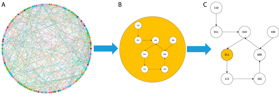
FIGURE 1. State change in a system: (A) all nodes’ state change, (B) one node of these nodes, and (C) the state change rule for one node, and there are eight states in these nodes.

Although given $\mathrm{ℰ}$, M, and the distribution $M_j$, it is not easy to figure out the particular states where the BNs are. The best probability of the distribution needs further calculation. Given Eq. 1, we can find that the more states in the system, the larger probability the states are. The probability of each distribution of the ensemble networks is proportional to the number of the BN state $\text{Ω}$. Thus, when determining the maximum probability, the maximum $\text{Ω}$ should be specified. Under the constrained conditions (2) and (3), we can use the differentiation to calculate the maximum value of the states. Two Lagrange multipliers α and ß will be utilized, and the condition of the peak can be written as follows:

$\frac{\partial }{\partial M_j}\text{lnΩ}-\alpha \frac{\partial {{\displaystyle \sum }}_j{M}_j}{\partial M_j}-\beta \frac{\partial {{\displaystyle \sum }}_j{M}_j{E}_j}{\partial M_j}=0.(7)$

To determine the probability, we need to assume that the number of M is relatively large. In contrast, the data of BNs do not need be large. When M goes to infinite, $M_j$ also goes to infinite. For $M\gg 1$, we can use the Stirring’s approximation to simulate $M!$

$M!={\left(\frac{M}{e}\right)}^M\sqrt{2\pi M}\left(1+\frac{1}{12M}+\frac{1}{288M}+\cdots \right).(8)$

Using Eq. 8 (the specific calculation process is shown in the Appendix), we can get the following equation:

$\text{ln}\text{Ω}=M\text{ln}M-M-{\displaystyle \sum }_j{M}_j\text{ln}{M}_j+{\displaystyle \sum }_j{M}_j.(9)$

When we compute the partial derivative of $\text{ln}\text{Ω}$, there are two ways to solve this problem (Eq. (8)), that is, one is fixing the M, while the other does not fix the M. The difference between the two solutions is a constant. In order to boost the computation, the second way for solving Eq. 9 is used.

$\frac{\partial \text{ln}\text{Ω}}{\partial M_j}=-\text{ln}{M}_j,(10)$

$\frac{\partial M}{\partial M_j}=1,(11)$

$\frac{\partial \mathrm{ℰ}}{\partial M_j}=E_j.(12)$

Substituting Eqs 10–12 into Eq. 7, we can get the following equations:

$-\text{ln}{M}_j-\alpha -\beta E_j=0,(13)$

$\text{ln}{M}_j=-\alpha -\beta E_j,(14)$

So there is

$M_j=e^{-\alpha -\beta E_j}.(15)$

When given the number of BN M, represented as the scale, we can get the distribution $M_j$, given that the parameters α and ß should be specified in advance. To prove Theorem 2, two definitions are given as follows.

Definition II1 When $P_j$ is the best probability distribution, the probability of system in the state j is

$P_j\equiv \frac{M_j}{M}=\frac{e^{-\beta E_j}}{{{\displaystyle \sum }}_j{e}^{-\beta E_j}}.(16)$

Definition II 2 Partition function [19] is

$Q\equiv {\displaystyle \sum }_j{e}^{-\beta E_j},(17)$

where Q indicates the sum of the probability of all the states. The partition of Eq. 17 plays an important role as a normalization constant.$E\equiv \frac{\mathrm{ℰ}}{M}$ and $E=\frac{1}{Q}{\displaystyle \sum }_j{E}_j{e}^{-\beta E_j}$ is the definition of E for succinctly, and the latter one in terms of formula expression is good for clarity and following computation.

After the computation of $P_j$, α can be eliminated, and ß can be expressed by the mean value E:

$E\equiv \frac{\mathrm{ℰ}}{M},(18)$

From Eq. 3, it can be rewritten as

$\begin{array}{cc}E& =\frac{{{\displaystyle \sum }}_j{M}_j{E}_j}{{{\displaystyle \sum }}_j{M}_j}\\ & =\frac{{{\displaystyle \sum }}_j{e}^{-\beta E_j}{E}_j}{{{\displaystyle \sum }}_j{e}^{-\beta E_j}}\end{array}.(19)$

Replacing Eq. 19 with Eq. 17, we can get

$E=\frac{1}{Q}{\displaystyle \sum }_j{E}_j{e}^{-\beta E_j}.(20)$

From the result, we can get the information about that in a canonical ensemble. When E is given, M tends to infinite, $P_j$ and ß do not have any relationship with M.

Theorem 2 When H and E are given and M tends to infinite, the best of the distribution M is the true distribution. In other words, the fluctuation is equal to 0.

Proof We need to talk about a function,

$f\equiv f\left(M_j\right)\equiv \text{ln Ω}-\alpha {\displaystyle \sum }_j{E}_j-\beta {\displaystyle \sum }_j{M}_j{E}_j.(21)$

However,

$\frac{{\partial }^{2}f}{\partial M_j^2}=\frac{{\partial }^2\text{ln Ω}}{\partial M_j^2}=-\frac{1}{M_j}<0.(22)$

Since the second term and the third term of f are the linear functions, the second derivative of $M_j$ equals to zero, which means the peak is stable.

Using the Taylor series which starts $f\left(M_j\right)$ at point $\overline{M_j}$, the equation can be obtained as follows:

$\begin{array}{l}f\left(M_j\right)=f\left(\overline{M_j}\right)+{\displaystyle \sum }_j\frac{\partial f}{\partial M_j}\left(M-\overline{M_j}\right)+{\displaystyle \sum }_j\frac{1}{2!}\frac{{\partial }^{2}f}{\partial M_j^2}{\left(M-\overline{M_j}\right)}^2+\cdots ,\\ =f\left(\overline{M_j}\right)-{\displaystyle \sum }_j\frac{\partial f}{\partial M_j}(M-\overline{M_j})+O\left(\frac{\text{Δ}M}{M}\right).p.\end{array}(23)$

The peak of f is as follows:

$\overline{f}=f\left(\overline{M_j}\right)=\ln \overline{\Omega }-\alpha M-\beta ME.(24)$

Substituting Eqs 21 and 24 into Eq. 23, we can get

$\ln \Omega =\ln \overline{\Omega }-{\displaystyle \sum }_j\frac{1}{2M{p}_j}{\left(M-\overline{M_j}\right)}^2+O\left(\frac{\text{Δ}M}{M}\right).(25)$

Ignoring the term $O\left(\frac{\text{Δ}M}{M}\right)$, we can get

$\text{ln}\frac{\text{Ω}}{\overline{\text{Ω}}}=-{\displaystyle \sum }_j\frac{1}{2M{p}_j}{\left(M-\overline{M_j}\right)}^2.(26)$

So there is

$\text{Ω}=\overline{\text{Ω}}{e}^{-{\displaystyle \sum }_j\frac{1}{2M{p}_j}{\left(M-\overline{M_j}\right)}^2}.(27)$

Thus, we complete the proof of this theorem.

2.3 The Fluctuation of the Distribution

This section is aiming to prove that cells are impossible in the same states, when the number of cells goes to infinity.

It is easy to find that Eq. 27 is a Gaussian distribution. Now, we need to prove the function Eq. 7 is a δ function. We need to prove the fluctuation would be eliminated when $M\to \infty$. Here, Theorem three is provided as follows:

Theorem 3 When $M\to \infty$, the value of fluctuation tends to be 0, that is,

$fluctuation\equiv \sqrt{\frac{\overline{M_j^2}-{\overline{M_j}}^2}{{\overline{M_j}}^2}}=\sqrt{\frac{M{P}_j}{{\left(M{P}_j\right)}^2}}\to 0.(28)$

Proof: There is a distribution that

$P\left(x\right)\propto e^{-\frac{x^2}{2{\text{Δ}}^2}}.$

Obviously, there is

$\overline{x}=0$

and

$\overline{x^2}=\frac{{\displaystyle \int x^2{e}^{-\frac{x^2}{2{\text{Δ}}^2}}}dx}{{\displaystyle \int e^{-\frac{x^2}{2{\text{Δ}}^2}}}dx}.(29)$

Then Eq. 29 can be rewritten as

$\begin{array}{c}\overline{x^2}=\frac{{\displaystyle \int x^2{e}^{-\frac{x^2}{2{\text{Δ}}^2}}}dx}{{\displaystyle \int e^{-\frac{x^2}{2{\text{Δ}}^2}}}dx}\\ =-2\frac{\partial }{\partial \left(\frac{1}{\frac{1}{{\text{Δ}}^2}}\right)}\text{ln}\left[{\displaystyle \int e^{-\frac{x^2}{2{\text{Δ}}^2}}}dx\right]\\ ={\text{Δ}}^3\frac{\partial }{\partial \left(\frac{1}{\text{Δ}}\right)}\text{ln Δ}\left[{\displaystyle \int e^{-\frac{x^2}{2}}}dx\right]\\ ={\text{Δ}}^3.\end{array}.(30)$

Comparing Eq. 27 with Eq. 30, we can get

${\left(M_j-\overline{M_j}\right)}^2=\overline{M_j^2}-{\overline{M_j}}^2=M{P}_j$

and substituting it into Eq. 28, there is

$fluctuation\equiv \sqrt{\frac{\overline{M_j^2}-{\overline{M_j}}^2}{{\overline{M_j}}^2}}=\sqrt{\frac{M{P}_j}{{\left(M{P}_j\right)}^2}}=\sqrt{\frac{1}{M{P}_j}}=0,$

where $M\to \infty$. Hence, the proof of the theorem is completed.

Until now, the proof of Theorem three is finished. When H and E are fixed and $M\to \infty$, the distribution with the maximum probability is the true distribution.

3 Experiments

In this section, we perform analysis of the cells’ states distribution model, that is, Eq 26. We establish that two experiments are conducted in order to illustrate the distribution of the BNs’ states, which can be used to verify our conclusions. Since there are no practical data for the state changes of the same type of cells, we can only simulate the transformation process of these cells through Boolean network, and then we also perform extensive analyses of the data of the state changes of these cells.

3.1 A Boolean Network with 100 Cells

In this example, we choose the state change function [17]. While the number of cells is 100, the number of the same Boolean is 1,000. And the Boolean network’s state change rule is illustrated as follows:

$\begin{array}{l}\{\begin{array}{cc}{x}_1\left(t+1\right)=x_1\left(t\right)\wedge x_2\left(t\right)& \\ x_2\left(t+1\right)=\mathrm{⌝}{x}_2\left(t\right)& \end{array},\\ \end{array}(31)$

where $\left(x_1,x_2\right)$ indicates the cell’s state, while $x=1$ or 0, and the function indicates the state change rule. Hence, in this example, there are four states in 100 cells, and the state change rule is shown in Figure 2B.

FIGURE 2

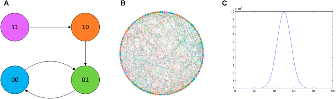
FIGURE 2. Cells of the system (31). The state change in the system (31), and the distribution of these states of combination. (A) Node’s states change, and there are four states in these cells; (B) the relation of 100 cells, and these cells were randomly generated; (C) main result of the system (31): the distribution of these states of combination.

Assume that the number of four initial states in the cells is shown in Table 1.

TABLE 1

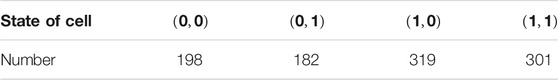
TABLE 1. Number of initial states of cells.

From Theorem 1, we can obtain the k combinations.

$k=\frac{1000!}{198!182!349!301!}=8.584\times {10}^{200}.$

We generate the particular network relationship between cells in a random manner, where each node represents a cell, and the edge indicates a connection between two cells. The probability of connecting the two cells is initialized as 0.05. The indicators of the association network between the cells are shown in the following table.

Through Figure 3; Table 2, we get the basic characteristics of this cellular network; there are 1,000 nodes, 2,781 edges, and so on. The visualization of the network is shown in Figure 2B. In this figure, different colors of the nodes are expressed as different states of the cells.

TABLE 2

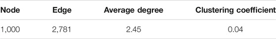
TABLE 2. Cellular network statistical characteristics.

FIGURE 3

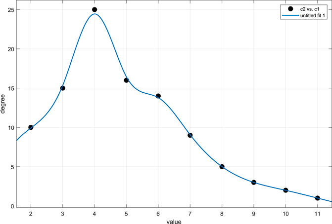
FIGURE 3. Distribution of the cellular network.

When the cell states change, they will be initialized with a random state, and the influence of states by other states is modeled as well. Assuming that the number of identical states between the connected cells is greater than 10, the other cells directly skip the changed state, and switch directly to the next state. Thus, the function $\text{Ω}$ can be obtained as follows:

$\text{Ω}=\overline{\text{Ω}}{e}^{-{\displaystyle \sum }_j\frac{1}{2M{p}_j}{\left(M-\overline{M_j}\right)}^2}.(32)$

where $\text{Ω}$ indicates the distribution, $P_i,i=\mathrm{1,2,3,4}$ is the probability of the cells state, M is the number of cells, and $\overline{M_j}$ is the number of jth states.

The state change rule as shown in Figure 2A demonstrates the end state is $\left(\mathrm{0,0}\right)$, meaning the cells getting the state $\left(\mathrm{0,0}\right)$ twice. In addition, the state of the cells will be randomly assigned, in Figure 2B, and it is easy to find that when $x=50$, the distribution reaches its mode, showing that when all the states of the cells are equal, the state in the collection of cells is the most prominent.

3.2 A Boolean Network with 150 Cells

In this example, we choose the state change function similar to the previous reported one [12]. Here, the number of cells is 500, meaning the number of the same Boolean is 500. Along with the Boolean network’s state change, the mathematical rules can be formatted as

$\{\begin{array}{cc}{x}_1\left(t+1\right)=x_2\left(t\right)\wedge x_3\left(t\right)& \\ x_2\left(t+1\right)=\mathrm{⌝}{x}_1\left(t\right)& \\ x_3\left(t+1\right)=x_2\left(t\right)\vee x_3\left(t\right)& \end{array}.(33)$

where $\left(x_1,x_2\right)$ mean the cell’s state, and $x=1$ or 0, and the function is the state change rule, so in this example, there are eight states in 450 cells, and the state change rule is shown in Figure 4B.

FIGURE 4

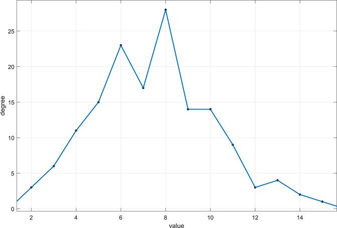
FIGURE 4. Distribution of the cellular network.

Assume that the number of four initial states in the cells is as shown in Table 3.

TABLE 3

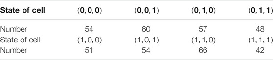
TABLE 3. Number of initial states of cells.

Form Theorem 1, we can get there are about k combinations.

$k=\frac{150!}{18!20!19!16!17!18!22!14!}=8.6616\times {10}^{367}.$

We generate a network relationship among cells in a random manner, where each node represents the cell, and the edge indicates that there is a connection between the two cells, and the probability of connecting the two cells is 0.05. The indicators of the association network between the cells are shown in the following Table 4.

TABLE 4

TABLE 4. Cellular network statistical characteristics.

Through Figure 4; Table 3, we get the basic characteristics of this cellular network; there are 450 nodes, 1890 edges, and so on. The visualization of the network is shown in Figure 5B. Here, different colors of the nodes are expressed as different states of the cells.

FIGURE 5

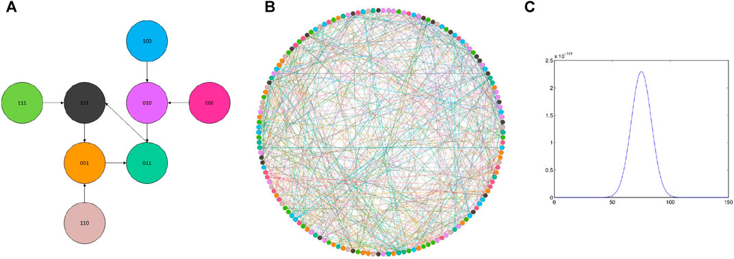
FIGURE 5. Cells of the system (33). State change in the system (33), and the distribution of these states of combination: (A) node’s state change, and there are eight states in these cells; (B) relation of 150 cells, and these cells were randomly generated; (C) result of the system (33): the distribution of these states of combination.

The state change rule as shown in Figure 5A, and the end state is $\left(\mathrm{0,0,1}\right)$, meaning the cells get the state $\left(\mathrm{0,0,1}\right)$ twice, and the state of the cells will be randomly assigned, in Figure 5B; it is easy to find that when $x\simeq 18$, the distribution reaches the peak. It means that when all the states of the cells are equal and the number of the eight states is approximately equal to 18, the collection of cells is the most prominent state.

From these two experiments, we verify that the distribution of these states is a Gaussian distribution, and these cells cannot be in the same state when the number of cells approaches to the infinity. Thus, the above theorems are right.

4 Conclusion

In this article, we study and calculate the distribution of the Boolean networks’ states. First, we compute the probability of different BNs’ states and get the value of $\text{Ω}$, then we find the maximum possible distribution of the number of BNs’ states. Furthermore, we calculate the fluctuation of the distribution. Finally, two representative experiments are conducted to verify the efficiency of the obtained results. Although the real genetic networks are different from the BNs, the theoretical and practical results in this study may be extended for more realistic models. Since the proposed algorithm is conceptually concise and efficient, it is highly extensible for various situations.

5 Data Availability Statement

The original contributions presented in the study are included in the article/Supplementary Material; further inquiries can be directed to the corresponding author.

6 Author Contributions

XC drafted the idea. ZL did the derivation, while BR drafted the manuscript. All authors have read through the manuscript.

7 Funding

This work was supported in part by National Natural Science Foundation of China (Grant Nos. 62003273, 62073263), Natural Science Foundation of Shaanxi Province (Grant No. 2020JQ-217), Fundamental Research Funds for the Central Universities (Grant No. 3102019HHZY03002).

Conflict of Interest

The authors declare that the research was conducted in the absence of any commercial or financial relationships that could be construed as a potential conflict of interest.

Publisher’s Note

All claims expressed in this article are solely those of the authors and do not necessarily represent those of their affiliated organizations, or those of the publisher, the editors and the reviewers. Any product that may be evaluated in this article, or claim that may be made by its manufacturer, is not guaranteed or endorsed by the publisher.

References

1. Ideker T, Galitski T, Hood L. A NEWAPPROACH TODECODINGLIFE: Systems Biology. Annu Rev Genom Hum Genet (2001) 2:343–72. doi:10.1146/annurev.genom.2.1.343

CrossRef Full Text | Google Scholar

2. Kim J, Park S-M, Cho K-H. Discovery of a Kernel for Controlling Biomolecular Regulatory Networks. Sci Rep (2013) 3:2223. doi:10.1038/srep02223

PubMed Abstract | CrossRef Full Text | Google Scholar

3. Zhang Z, Xia C, Chen Z. On the Stabilization of Nondeterministic Finite Automata via Static Output Feedback. Appl Math Comput (2020) 365:124687. doi:10.1016/j.amc.2019.124687

CrossRef Full Text | Google Scholar

4. Shmulevich I, Dougherty ER, Kim S, Zhang W. Probabilistic Boolean Networks: a Rule-Based Uncertainty Model for Gene Regulatory Networks. Bioinformatics (2002) 18(2):261–74. doi:10.1093/bioinformatics/18.2.261

PubMed Abstract | CrossRef Full Text | Google Scholar

5. Liang J, Han J. Stochastic Boolean Networks: An Efficient Approach to Modeling Gene Regulatory NetworksBMC Syst Biol (2012) 6:113. doi:10.1186/1752-0509-6-113

PubMed Abstract | CrossRef Full Text

6. Peican Zhu P, Jie Han J. Stochastic Multiple-Valued Gene Networks. IEEE Trans Biomed Circuits Syst (2014) 8(1):42–53. doi:10.1109/tbcas.2013.2291398

PubMed Abstract | CrossRef Full Text | Google Scholar

7. Kauffman SA. Metabolic Stability and Epigenesis in Randomly Constructed Genetic Nets. J Theor Biol (1969) 22:437–67. doi:10.1016/0022-5193(69)90015-0

CrossRef Full Text | Google Scholar

8. Kauffman SA. The Origins of Order. Self-Organization and Selection in Evolution. Oxford University Press (1993).

Google Scholar

9. Zhu P, Liang J, Han J. Gene Perturbation and Intervention in Context-Sensitive Stochastic Boolean Networks. BMC Syst Biol (2014) 8–60. doi:10.1186/1752-0509-8-60

CrossRef Full Text | Google Scholar

10. Zhu P, Han J. Asynchronous Stochastic Boolean Networks as Gene Network Models[J]. J Compu. Biol. (2014) 21(10):771–83. doi:10.1089/cmb.2014.0057

CrossRef Full Text | Google Scholar

11. Cheng D. Analysis and Control of Boolean Networks: A Semi-Tensor Product Approach[M]. Berlin: Springer (2010).

Google Scholar

12. Cheng D, Qi H. A Linear Representation of Dynamics of Boolean Networks. IEEE Trans Automat Contr (2010) 55:2251–8. doi:10.1109/tac.2010.2043294

CrossRef Full Text | Google Scholar

13. Li R, Yang M, Chu T. State Feedback Stabilization for Boolean Control Networks. IEEE Trans Automat Contr (2013) 58:1853–7. doi:10.1109/tac.2013.2238092

CrossRef Full Text | Google Scholar

14. Li B, Lu J, Liu Y, Wu Z-G. The Outputs Robustness of Boolean Control Networks via Pinning Control. IEEE Trans Control Netw Syst (2020) 7(1):201–9. doi:10.1109/tcns.2019.2913543

CrossRef Full Text | Google Scholar

15. Liu A, Li H. On Feedback Invariant Subspace of Boolean Control Networks. Sciece China Inf Sci (2020) 63(12):229201. doi:10.1007/s11432-019-9869-6

CrossRef Full Text | Google Scholar

16. Zhang Z, Xia C, Chen S, Yang T, Chen Z. Reachability Analysis of Networked Finite State Machine with Communication Losses: A Switched Perspective. IEEE J Select Areas Commun (2020) 38(5):845–53. doi:10.1109/jsac.2020.2980920

CrossRef Full Text | Google Scholar

17. Laschov D, Margaliot M. Observability of Boolean Networks: A Graph-Theoretic Approach. Cambridge, U.K.: Cambridge Scientific Publishers, Cambridge (2013).

Google Scholar

18. Laschov D, Margaliot M. A Maximum Principle for Single-Input Boolean Control Networks. IEEE Trans Automat Contr (2011) 56:913–7. doi:10.1109/tac.2010.2101430

CrossRef Full Text | Google Scholar

19. Baxter RJ. Partition Function of the Eight-Vertex Lattice Model. Ann Phys (2000) 281(1-2):187–222. doi:10.1006/aphy.2000.6010

CrossRef Full Text | Google Scholar

Appendix

Logarithm Eq. 4, we can get

$\begin{array}{ll}\ln \Omega \hfill & =\text{ln}M!-\left({\ln \Pi }_j{M}_j!\right)\hfill \\ \hfill & =\text{ln}M!-{\displaystyle \sum }_{j}ln{M}_j\hfill \end{array}.$A1

Replacing Eq. A2 with Eq. 8, we can get

$\begin{array}{ll}\ln \Omega \hfill & =\text{ln}{\left(\frac{M}{e}\right)}^M\sqrt{2\pi M}(1+\frac{1}{12M}+\frac{1}{288M+\dots })\hfill \\ \hfill & -{\displaystyle \sum }_j\text{ln}{\left(\frac{M_j}{e}\right)}^{M_j}\sqrt{2\pi M_j}(1+\frac{1}{12M_j}+\frac{1}{288M_j+\dots })\hfill \\ \hfill & =M\text{ln}M-M+ln\sqrt{2\pi M}\left(1+\frac{1}{12M}+\frac{1}{288M+\dots }\right)\hfill \\ \hfill & -{\displaystyle \sum }_j{M}_j\text{ln}{M}_j-M_j+ln\sqrt{2\pi M_j}(1+\frac{1}{12M_j}+\frac{1}{288M+\dots })\hfill \\ \hfill & =M\text{ln}M-M-{\displaystyle \sum }_j{M}_j\text{ln}{M}_j-{\displaystyle \sum }_j{M}_j+ln\frac{\sqrt{2\pi M_j}\left(1+\frac{1}{12M_j}+\frac{1}{288M_j+\dots }\right)}{{{\displaystyle \sum }}_{j}ln\sqrt{2\pi M_j}\left(1+\frac{1}{12M_j}+\frac{1}{288M+\dots }\right)}\hfill \\ \hfill & =M\text{ln}M-M-{\displaystyle \sum }_j{M}_j\text{ln}{M}_j-{\displaystyle \sum }_j{M}_j\hfill \end{array}.$A2