A Bistable Phenomena Induced by a Mean-Field SIS Epidemic Model on Complex Networks: A Geometric Approach

In this paper, we propose a degree-based mean-field SIS epidemic model with a saturated function on complex networks. First, we adopt an edge-compartmental approach to lower the dimensions of such a proposed system. Then we give the existence of the feasible equilibria and completely study their stability by a geometric approach. We show that the proposed system exhibits a backward bifurcation, whose stabilities are determined by signs of the tangent slopes of the epidemic curve at the associated equilibria. Our results suggest that increasing the management and the allocation of medical resources effectively mitigate the lag effect of the treatment and then reduce the risk of an outbreak. Moreover, we show that decreasing the average of a network sufficiently eradicates the disease in a region or a country.

1 Introduction

Mathematical modeling plays a crucial role in fighting against large scale infectious disease such as Tuberculosis, HIV, COVID-19, etc., Compartment models have been used to anticipate the progression of diseases and evaluate the effect of interventions on disease spread [1]. One of such models separates the total population into two distinct categories with respect to disease status. People who have not gotten the disease are labeled “susceptibles”; while those who have been infected by a certain disease are called “infectives”. This kind of compartment model is denoted by “an SIS epidemic model” [2–7], which has been extensively used to address the dynamics of those diseases, describing an individual infected by a disease as having no immunity, thus becoming a susceptible again.

Most of the existing models assume that all the individuals are well-mixed and they have homogeneous mixing of surfaces, which implies that each individual has the same probability to contact other individuals and ignores the degree of social heterogeneity induced by age, household, spatial structures, and social spheres, etc. Generally, the social interactions of individuals generate a certain pattern based on social preferences, which contributes to transmission heterogeneity. Indeed, such factors may play a decisive role in the disease transmission and they also may help health policymakers to take more effective control measures for curbing the disease spread [7, 8]. Epidemic models on complex networks incorporate such contact heterogeneity and take account for how the structures of the networks affect the disease prevalence. A popular degree-based SIS epidemic model has been built [9] and it exhibits threshold dynamics [4, 5]. Since then, many factors including vector-borne [10, 11], infective media [12], awareness reaction [13], and the gene diversity of pathogens [14], etc., have been incorporated into the study of the co-evolution of networks and epidemics.

In epidemiology, the basic reproduction number, ${\mathrm{ℛ}}_0$, denotes the average number of secondary cases produced by a typical disease carrier during their infectious period [15–17]. Generally, if ${\mathrm{ℛ}}_0<1,$ the infection will be eradicated as each infected individual suffers a disease, on average, to less than one other individual; if it is greater than one, then the outbreak will grow exponentially. For a degree-based SIS epidemic model, the expression of the basic reproduction number is given by

${\mathrm{ℛ}}_0=\frac{\beta }{\gamma }\frac{\langle k^2\rangle }{\langle k\rangle },\langle k^2\rangle ={\displaystyle \sum }_{k=1}^n{k}^{2}p\left(k\right),\langle k\rangle ={\displaystyle \sum }_{k=1}^{n}kp\left(k\right),$

with transmission rate β and treatment rate $\gamma ,$ which serves a vital role in mitigating a disease transmission. However, when people face an emerging infectious disease, such as COVID-19, SARS, H1N1 etc., it may lead to a sharp increase in the number of patients and may cause serious runs of medical resources. A delay phenomena occurs since some infected individuals can not be instantly treated in hospitals. Such properties can be addressed by a Hill function by

$T\left(I\right)=\frac{\gamma I}{1+\alpha I}.$

where α denotes a hysteretic effect due to medical limitations. Apparently, $T\left(I\right)\to 0$ when I is small enough and it tends towards to $\gamma /\alpha$ when I is large enough. The constant $\gamma /\alpha$ represents the capacity for treatment. Some scholars proposed a type of step function [18] and a Verhulst-type function [19], which have similar properties to $T\left(I\right)$.

In view of such epidemiological models incorporating a saturated treatment function, it is not hard to find that most of them enable such models, essentially changing their dynamics. Once a saturated function has been introduced, there always exists a backward bifurcation, which implies that even if some certain control measures make ${\mathrm{ℛ}}_0<1$, it does not guarantee the eradication of a disease in a region or a county. The presence of a backward bifurcation indicates that there exists a bistable phenomena, i.e, a stable endemic equilibria and a stable disease-free equilibrium coexist when ${\mathrm{ℛ}}_0<1.$ The epidemic curve converging to zero or a positive constant is definitely determined by initial sizes of an infection. Some other epidemiological mechanisms, including partial immunity by vaccination [20], death caused by the disease [21], and susceptible heterogeneity [22] etc., have been identified to produce a backward bifurcation. However, the existing results are usually shown in homogeneous models. Up to date, there are few results to study backward bifurcation phenomena in epidemic models on complex networks from theoretical view of points. Recently, Li and Yousef proposed two degree-based SIR and SIS models with a saturated function to study a backward bifurcation phenomena. They showed a sufficient condition for the occurrence of a backward bifurcation [23, 24]. Indeed, since network models have higher dimensions than those of well-mixed models, studying the complex dynamics of such models is a challenging issue from a theoretical view of points.

There are three main contributions in this paper. First, we propose a degree-based SIS epidemic model with a saturated function to study its long-term behaviors. Second, to overcome the difficulty of high dimensions for a network, we adopt an edge-based compartmental approach to lower the dimensions of an SIS epidemic model. Such an approach changes a complete degree-based model to a degree-edge-mixed model, and hence, it lowers the dimension of such a model from $2n$ to $n+1.$ Third, we proposed a geometric method to completely characterize the local stability of each equilibrium.

The organization of this paper is as follows: In Section 2, a degree-based SIS epidemic model on complex networks with a saturated function is proposed. Furthermore, we adopt an edge-compartmental approach to rewrite it as a degree-edge-mixed model. Section 3 gives a geometric approach to study the local stability of each equilibrium. In Section 4, we conducted some numerical simulations to illustrate our theoretical results. We give a brief discussion in the last section.

2 Model Formulation

In this paper, we focus on the complete stability of each equilibrium by a novel approach. Let us assume that the maximum contact number of an individual is n and then the degree set is $\mathrm{\mathbb{N}}=\left\{\mathrm{1,2},\cdots ,n\right\}.$ The total subpopulation $N_k\left(t\right)$ is categorized into two statuses: susceptible and infective. Let $S_k\left(t\right)$ and $I_k\left(t\right)$ represent the densities of susceptible nodes and infected nodes at time t and degree $k(k\in \mathrm{\mathbb{N}})$, respectively. Inspired by the modeling approach [9], we account for the limitation of medical resources and propose a mean-field SIS epidemic model as follows:

$\{\begin{array}{l}\frac{d{S}_k\left(t\right)}{dt}=-\beta k{S}_k\left(t\right)\text{Θ}\left(t\right)+\frac{\gamma I_k\left(t\right)}{1+\alpha \text{Θ}\left(t\right)},\\ \frac{d{I}_k\left(t\right)}{dt}=\beta k{S}_k\left(t\right)\text{Θ}\left(t\right)-\frac{\gamma I_k\left(t\right)}{1+\alpha \text{Θ}\left(t\right)},\end{array}(1)$

where β denotes the transmission rate and γ represents the treatment rate; α stands for the lag effect of the treatment due to the limitation of medical resources. From epidemiological view of points, the term

$\text{Θ}\left(t\right)=\frac{1}{\langle k\rangle }{\displaystyle \sum }_{k=1}^{n}kp\left(k\right)I_k\left(t\right),$

denotes the probability of a given node connecting to an infected node at time t. Hence, it can be considered as a density of an $\left[SI\right]$ edge at time t. Following the steps [10], model (1) can be rewritten as a degree-edge-mixed mode.

$\{\begin{array}{l}\frac{d{S}_k\left(t\right)}{dt}=-\beta k{S}_k\left(t\right)\text{Θ}\left(t\right)+\frac{\gamma \left[1-S_k\left(t\right)\right]}{1+\alpha \text{Θ}\left(t\right)},\\ \frac{d\text{Θ}\left(t\right)}{dt}=\frac{1}{\langle k\rangle }{\displaystyle \sum }_{k=1}^n\hspace{0.17em}\beta k^{2}p\left(k\right)S_k\left(t\right)\text{Θ}\left(t\right)-\frac{\gamma \hspace{0.17em}\text{Θ}\left(t\right)}{1+\alpha \text{Θ}\left(t\right)},\end{array}(2)$

with initial condition

$S_k\left(0\right)=S_{k0}>0,\text{Θ}\left(0\right)={\text{Θ}}_0\ge 0.$

Lemma 2.1. If $\text{Θ}\left(0\right)>0,$ system (2) has a positive solution, i.e, for all $k\in \mathrm{\mathbb{N}}$ and $t\in {\mathrm{ℝ}}_{+},$$S_k\left(t\right)>0$ and $\text{Θ}\left(t\right)>0.$Proof Observing the $\left(n+1\right)$ equation of system (2), we solve it and obtain

$\text{Θ}\left(t\right)=\text{Θ}\left(0\right)e^{{\displaystyle {\int }_0^{t}z\left(\tau \right)d\tau }},(3)$

where

$z\left(t\right)=\frac{\beta }{\langle k\rangle }{\displaystyle \sum }_{k=1}^n{k}^{2}p\left(k\right)S_k\left(t\right)-\frac{\gamma }{1+\alpha \text{Θ}\left(t\right)}.$

Obviously, $\text{Θ}\left(t\right)>0$ if $\text{Θ}\left(0\right)>0.$ Now, we will prove the positivity of $S_k\left(t\right)$ for $k\in \mathrm{\mathbb{N}}$ and $t\in {\mathrm{ℝ}}_{+}.$ By the continuity of the solution, if we claim that there exists a $t_0>0$ such that $S_k\left(t_0\right)=0$ for some $k\in \mathrm{\mathbb{N}}$. Then $S_k\left(t\right)>0$ for $t\in [0,t_0)$ and $S_k\text{′}\left(t_0\right)<0.$ However, from the first n equation of (2), it follows that

$\frac{d{S}_k\left(t\right)}{dt}{|}_{t=t_0}=\frac{\gamma }{1+\alpha \text{Θ}\left(t_0\right)}>0.$

This leads to a contradiction with the claim. Therefore, $S_k\left(t\right)>0$ for $k\in {\mathrm{\mathbb{N}}}_{+}$ and $t\in {\mathrm{ℝ}}_{+}$.

Remark 2.1. Lemma 2.1 ensures that the solution of system (2) is strictly positive if${\text{Θ}}_0>0$, which supports that$I_k\left(t\right)>0$for all$t\in {\mathrm{ℝ}}_{+}$and$k\in \mathrm{\mathbb{N}}.$The strong connectivity of a network guarantees the positivity of the solution as long as$I_k\left(0\right)\cancel{\ne }0$or there exists at least$k_0\in \mathrm{\mathbb{N}}$such that$I_{k_0}>0.$Noting that $N_k\left(t\right)=S_k\left(t\right)+I_k\left(t\right)=1,$ we have from Lemma 2.1 that $S_k\left(t\right)\le 1,$ and $I_k\left(t\right)<1,$ for all $k\in \mathrm{\mathbb{N}}$ and $t\in {\mathrm{ℝ}}_{+}.$ Employing the expression of $\text{Θ}$, we assert that

$\text{Θ}\left(t\right)=\frac{1}{\langle k\rangle }{\displaystyle \sum }_{k=1}^{n}kp\left(k\right)I_k\left(t\right)<1.$

Therefore, for all $t\in {\mathrm{ℝ}}_{+}$ and $k\in \mathrm{\mathbb{N}}$, the set

$\text{Γ}=\{\varphi \in {\left({\mathrm{ℝ}}_{+}\right)}^{n+1}|0<S_k\left(t\right)\le \mathrm{1,0}\le \text{Θ}\left(t\right)<1\}(4)$

is positively invariant associate with system (2) and $\varphi =\left(S_{k0},{\text{Θ}}_0\right).$ In what follows, we focus on the long term behaviors of system (2) taking the initial data from $\text{Γ}$.

3 Stability of Equilibria

In this section, we will consider the local stability of system (2) by a novel-geometric approach, which resolves such a matter once and for all. First, we try to give the basic reproduction number ${\mathrm{ℛ}}_0$ in an explicit form by the approach in [25]. Obviously, system (2) always has a disease-free equilibrium $E_0=\left(\mathrm{1,0}\right)$. Linearising the $n+1$ equation in system (2) yields to

$\frac{d\text{Θ}\left(t\right)}{dt}=\frac{\beta \langle k^2\rangle }{\langle k\rangle }\text{Θ}\left(t\right)-\gamma \hspace{0.17em}\text{Θ}\left(t\right),(5)$

Solving Eq. 5 by a constant variation method, one drives a renew equation

$\text{Θ}\left(t\right)={\text{Θ}}_0{e}^{-\gamma t}+\frac{\beta \langle k^2\rangle }{\langle k\rangle }{\displaystyle {\int }_0^t{e}^{-\gamma \hspace{0.17em}\tau }}\text{Θ}\left(t-\tau \right)d\tau .(6)$

So that the basic reproduction number is calculated in form of

${\mathrm{ℛ}}_0=\frac{\langle k^2\rangle }{\langle k\rangle }\frac{\beta }{\gamma }.(7)$

The epidemiological meaning of ${\mathrm{ℛ}}_0$ is the average number of secondary infected edges produced by a typical $\left[SI\right]$ edge during its infectious period. Now, let us account for the local stability of disease-free equilibrium $E_0$.

Theorem 3.1. If ${\mathrm{ℛ}}_0<1,$ then the disease-free equilibrium $E_0$ is locally asymptotically stable for any $\varphi \in \text{Γ}.$Proof Linearizing system (2) around the disease-free equilibrium $E_0$ results in

$\{\begin{array}{cc}\frac{d{s}_k\left(t\right)}{dt}=& -\gamma s_k\left(t\right)-\beta k{S}_k^0\theta ,\\ \frac{d\theta \left(t\right)}{dt}=& \left(\frac{\beta \langle k^2\rangle }{\langle k\rangle }-\gamma \right)\theta .\end{array}(8)$

Let us assume that system (8) has the solution with exponential forms, i.e, $s_k\left(t\right)=s_{k0}{e}^{\mathrm{\lambda }t}$ and $\theta \left(t\right)={\theta }_0{e}^{\lambda t}.$ Plugging them into (8), we have that

$\{\begin{array}{cc}\mathrm{\lambda }{s}_{k0}=& -\gamma s_{k0}-\beta k{\theta }_0,\\ \mathrm{\lambda }{\theta }_0=& \left(\frac{\beta \langle k^2\rangle }{\langle k\rangle }-\gamma \right){\theta }_0,\end{array}(9)$

If ${\theta }_0\ne 0$, we cancel ${\theta }_0$ on both sides of system (8) to derive that $\mathrm{\lambda }=\gamma \left({\mathrm{ℛ}}_0-1\right).$ Otherwise, ${\theta }_0=0.$ From the first equation of (8), it follows that $\mathrm{\lambda }=-\gamma <0.$ From what has been discussed, we conclude that if ${\mathrm{ℛ}}_0<1,$ then the disease-free equilibrium $E_0$ is locally stable for any $\varphi \in \text{Γ}.$

Theorem 3.2. If $\widehat{{\mathrm{ℛ}}_0}=\frac{\beta \left(1+\alpha \right)\langle k^2\rangle }{\gamma \langle k\rangle }\le 1,$ the disease-free equilibrium $E_0$ is globally asymptotically stable if $\varphi \in \text{Γ}.$Proof Let us candidate a Lyapunov function by

$V\left(t\right)=\text{Θ}\left(t\right).$

Differentiating V along the solution of system (2) leads to

$\begin{array}{c}\frac{dV\left(t\right)}{dt}{|}_{\left(2\right)}=\frac{d\text{Θ}\left(t\right)}{dt}=\frac{1}{\langle k\rangle }\stackrel{n}{{\displaystyle \sum }_{k=1}}\beta k^{2}p\left(k\right)S_k\left(t\right)\text{Θ}\left(t\right)-\frac{\gamma \text{Θ}\left(t\right)}{1+\alpha \text{Θ}\left(t\right)}\\ \le \left(\frac{\beta \langle k^2\rangle }{\langle k\rangle }-\frac{\gamma }{1+\alpha \text{Θ}}\right)\text{Θ}\left(t\right)\\ =\left(\frac{\beta \langle k^2\rangle }{\langle k\rangle }-\frac{\gamma }{1+\alpha }-\frac{\gamma \alpha \left(1-\text{Θ}\left(t\right)\right)}{\left(1+\alpha \right)\left(1+\alpha \text{Θ}\left(t\right)\right)}\right)\text{Θ}\left(t\right)\\ <\left(\frac{\beta \langle k^2\rangle }{\langle k\rangle }-\frac{\gamma }{1+\alpha }\right)\text{Θ}\left(t\right)\\ =\frac{\gamma }{1+\alpha }\left(\widehat{{\mathrm{ℛ}}_0}-1\right)\text{Θ}\left(t\right),\end{array}$

here we have used the fact that $\text{Θ}\left(t\right)<1$ and $S_k\left(t\right)\le 1$ for all $t\in {\mathrm{ℝ}}_{+}.$ Hence, if $\widehat{{\mathrm{ℛ}}_0}<1,$ then $\dot{V\left(t\right)}<0.$ While if $\widehat{{\mathrm{ℛ}}_0}=1,$ then

$\frac{dV\left(t\right)}{dt}{|}_{\left(2\right)}\le -\frac{\gamma \alpha \left(1-\text{Θ}\left(t\right)\right)}{\left(1+\alpha \right)\left(1+\alpha \text{Θ}\left(t\right)\right)}\text{Θ}\left(t\right)\le 0.$

The equality holds if and only if $\text{Θ}\left(t\right)=0.$ Hence, the largest invariant set $M=\{\varphi \in \text{Γ}|\dot{V\left(t\right)}=0\}$ only contains a singleton point $E_0.$ Consequently, the Lyapunov-Kasovskii-LaSalle theorem ensures that $E_0$ is globally asymptotically stable if $\widehat{{\mathrm{ℛ}}_0}<1.$Now, we are in a position to study the existence of the endemic steady state, whose components of that feasible equilibrium satisfy

$\{\begin{array}{cc}0=& -\beta k{S}_k^{\text{*}}{\text{Θ}}^{\text{*}}+\frac{\gamma \left(1-S_k^{\text{*}}\right)}{1+\alpha {\text{Θ}}^{\text{*}}},\\ 0=& \frac{1}{\langle k\rangle }{\displaystyle \sum }_{k=1}^n\beta k^{2}p\left(k\right)S_k^{\text{*}}{\text{Θ}}^{\text{*}}-\frac{\gamma {\text{Θ}}^{\text{*}}}{1+\alpha {\text{Θ}}^{\text{*}}}.\end{array}(10)$

From the first equation of (10), we get

$S_k^{\text{*}}=\frac{\frac{\gamma }{1+\alpha {\text{Θ}}^{\text{*}}}}{\beta k{\text{Θ}}^{\text{*}}+\frac{\gamma }{1+\alpha {\text{Θ}}^{\text{*}}}},k\in \mathrm{\mathbb{N}}.(11)$

Substituting Eq. 11 into the second equation of (10) and canceling $\frac{\gamma {\text{Θ}}^{\text{*}}}{1+\alpha {\text{Θ}}^{\text{*}}}$, we have that

$F\left({\text{Θ}}^{\text{*}}\right):=1-\frac{\beta }{\langle k\rangle }{\displaystyle \sum }_{k=1}^n{k}^{2}p\left(k\right)\frac{1}{\beta k{\text{Θ}}^{\text{*}}+\frac{\gamma }{1+\alpha {\text{Θ}}^{\text{*}}}}.(12)$

Apparently, if $F\left(\text{Θ}\right)=0$ has a solution $\text{Θ}>0$, then system (10) has an endemic equilibrium. Note that $F\left(\text{Θ}\right)$ has the following properties:

$F\left(0\right)=1-{\mathrm{ℛ}}_0,F\left(1\right)=1-\frac{\beta }{\langle k\rangle }\stackrel{n}{{\displaystyle \sum }_{k=1}}{k}^{2}p\left(k\right)\frac{1}{\beta k+\frac{\gamma }{1+\alpha }}>0.(13)$

Consequently, we conclude the following theorem on the existence of system (2).

Theorem 3.3 If ${\mathrm{ℛ}}_0>1,$ then $F\left(\text{Θ}\right)$ has at least one positive solution ${\text{Θ}}^{\text{*}}.$ In turn, system (2) has at least one positive endemic equilibrium $E^{\text{*}}.$

Proof If ${\mathrm{ℛ}}_0>1,$ then $F\left(0\right)<0$ and $F\left(1\right)>0.$ The Immediate Value Theorem ensures that $F\left({\text{Θ}}^{\text{*}}\right)=0$ has at least one positive point in $\left(\mathrm{0,1}\right).$

From Theorem 3.3, we assert that system (2) has the existence of the endemic equilibrium, but it does not guarantee the uniqueness of the positive solution when ${\mathrm{ℛ}}_0>1.$ However, if α is too small or large enough, it is easy to find that the function F is a decreasing function associated with $\text{Θ}.$ Then we can claim the uniqueness of the endemic equilibrium whereas ${\mathrm{ℛ}}_0>1.$ However, for ${\mathrm{ℛ}}_0<1,$ we do not catch the existence of such equilibria due to the complex structure of $F.$ To overcome that difficulty, we select a sensitive analysis for model parameters to investigate the existence of a backward bifurcation of that model for ${\mathrm{ℛ}}_0<1.$

Now, we are concerned with the endemic curve which bifurcates backwards at $\left({\mathrm{ℛ}}_0,{\text{Θ}}^{\text{*}}\right)=\left(\mathrm{1,0}\right).$ If a backward bifurcation takes place, there always exist some additional conditions except ${\mathrm{ℛ}}_0<1.$ To assess such a phenomena, we express $\beta ={\mathrm{ℛ}}_0\gamma \frac{\langle k\rangle }{\langle k^2\rangle }$ from ${\mathrm{ℛ}}_0.$ Substituting this expression into Eq. 12, one arrives at

$F\left({\text{Θ}}^{\text{*}}\right)=1-{\mathrm{ℛ}}_0\langle k^2\rangle \stackrel{n}{{\displaystyle \sum }_{k=1}}{k}^{2}p\left(k\right)\frac{1}{{\mathrm{ℛ}}_0\frac{\langle k\rangle }{\langle k^2\rangle }k{\text{Θ}}^{\text{*}}+\frac{1}{1+\alpha {\text{Θ}}^{\text{*}}}}=0.(14)$

Calculating the derivative of Eq. 14 with respect to ${\mathrm{ℛ}}_0$ by the Implicit Function Theorem, we obtain

$\frac{\partial {\text{Θ}}^{\text{*}}}{\partial {\mathrm{ℛ}}_0}=\frac{{{\displaystyle \sum }}_{k=1}^n{k}^{2}p\left(k\right)\tau \left(k,{\mathrm{ℛ}}_0,{\text{Θ}}^{\text{*}}\right)\left[1-{\mathrm{ℛ}}_0\tau \left(k,{\mathrm{ℛ}}_0,{\text{Θ}}^{\text{*}}\right)Q\left(k,{\mathrm{ℛ}}_0,{\text{Θ}}^{\text{*}}\right)\right]}{{\mathrm{ℛ}}_0{{\displaystyle \sum }}_{k=1}^n{k}^{2}p\left(k\right)M\left(k,{\mathrm{ℛ}}_0,{\text{Θ}}^{\text{*}}\right){\tau }^2\left(k,{\mathrm{ℛ}}_0,{\text{Θ}}^{\text{*}}\right)},(15)$

where

$\begin{array}{l}\tau \left(k,{\mathrm{ℛ}}_0,\text{Θ}\right)=\frac{1}{{\mathrm{ℛ}}_0\frac{\langle k\rangle }{\langle k^2\rangle }k\text{Θ}+\frac{1}{1+\alpha \text{Θ}}},\\ M\left(k,{\mathrm{ℛ}}_0,\text{Θ}\right)=k{\mathrm{ℛ}}_0\frac{\langle k\rangle }{\langle k^2\rangle }-\frac{\alpha }{{\left(1+\alpha \text{Θ}\right)}^2},\\ Q\left(k,{\mathrm{ℛ}}_0,\text{Θ}\right)=k\frac{\langle k\rangle }{\langle k^2\rangle }\text{Θ}.\end{array}$

After a simple computation, we have that

$\frac{\partial {\text{Θ}}^{\text{*}}}{\partial {\mathrm{ℛ}}_0}{|}_{\left({\mathrm{ℛ}}_0,\text{Θ}\right)=\left(\mathrm{1,0}\right)}=\frac{{\langle k^2\rangle }^2}{\langle k\rangle \langle k^3\rangle -\alpha {\langle k^2\rangle }^2}.(16)$

Lemma 3.4. Suppose ${\mathrm{ℛ}}_0<1.$ A backward bifurcation occurs if the following inequality holds:

$\alpha >\frac{\langle k\rangle \langle k^3\rangle }{{\langle k^2\rangle }^2}.(17)$

Proof This is a direct result from Section 2.3 [26].Next, let us move our attention on to the local stability of equilibria if they exist, which is a challenge issue for a degree-based epidemic model due to the complex structure. We will propose a geometric approach to deal with such an issue.Linearising system (2) around $E^{\text{*}}$ and taking the exponential perturbation solution similar to Theorem 3.1, we obtain

$\left(\mathrm{\lambda }+\beta k{\text{Θ}}^{\text{*}}+\frac{\gamma }{1+\alpha {\text{Θ}}^{\text{*}}}\right)s_{k0}+\left(\beta k{S}_k^{\ast }+\frac{\alpha \gamma \left(1-S_k^{\text{*}}\right)}{{\left(1+\alpha {\text{Θ}}^{\text{*}}\right)}^2}\right){\theta }_0=0,(18)$

$-\frac{1}{\langle k\rangle }{\displaystyle \sum _{k=1}^n\beta k^{2}p\left(k\right){\text{Θ}}^{\text{*}}{s}_{k0}}+\left(\mathrm{\lambda }+\frac{\gamma }{{\left(1+\alpha {\text{Θ}}^{\text{*}}\right)}^2}-\frac{1}{\langle k\rangle }{\displaystyle \sum \beta k^{2}p\left(k\right)S_k^{\text{*}}}\right){\theta }_0=0(19)$

If $\mathrm{\lambda }\ne -\left(\beta k{\text{Θ}}^{\text{*}}+\frac{\gamma }{1+\alpha {\text{Θ}}^{\text{*}}}\right),$ solving Eq. 18 yields to

$s_{k0}=-\frac{\left(\beta k{S}_k^{\text{*}}+\frac{\alpha \gamma \left(1-S_k^{\text{*}}\right)}{{\left(1+\alpha {\text{Θ}}^{\text{*}}\right)}^2}\right){\theta }_0}{\mathrm{\lambda }+\beta k{\text{Θ}}^{\text{*}}+\frac{\gamma }{1+\alpha {\text{Θ}}^{\text{*}}}}.(20)$

Replacing $s_{k0}$ in Eq. 19 by Eq. 20 and canceling ${\theta }_0$, one admits

$H\left(\mathrm{\lambda }\right)=:\frac{\beta {\text{Θ}}^{\text{*}}}{\langle k\rangle }\stackrel{n}{{\displaystyle \sum }_{k=1}}{k}^{2}p\left(k\right)\frac{\beta k{S}_k^{\text{*}}+\frac{\alpha \gamma \left(1-S_k^{\text{*}}\right)}{{\left(1+\alpha {\text{Θ}}^{\text{*}}\right)}^2}}{\mathrm{\lambda }+\beta k{\text{Θ}}^{\text{*}}+\frac{\gamma }{1+\alpha {\text{Θ}}^{\text{*}}}}+\mathrm{\lambda }+\frac{\gamma }{{\left(1+\alpha {\text{Θ}}^{\text{*}}\right)}^2}-\frac{\beta }{\langle k\rangle }\stackrel{n}{{\displaystyle \sum }_{k=1}}{k}^{2}p\left(k\right)S_k^{\text{*}}=0.(21)$

Recall that

$\frac{\beta }{\langle k\rangle }{\displaystyle \sum }_{k=1}^n{k}^{2}p\left(k\right)S_k^{\text{*}}=\frac{\gamma }{1+\alpha {\text{Θ}}^{\text{*}}},$

and hence,

$\begin{array}{c}H\left(0\right)=\frac{\beta }{\langle k\rangle }\stackrel{n}{{\displaystyle \sum }_{k=1}}{k}^{2}p\left(k\right)\frac{\beta k{S}_k^{\text{*}}{\text{Θ}}^{\text{*}}+\frac{\gamma \alpha \left(1-S_k^{\text{*}}\right){\text{Θ}}^{\text{*}}}{{\left(1+\alpha {\text{Θ}}^{\text{*}}\right)}^2}}{\beta k{\text{Θ}}^{\text{*}}+\frac{\gamma }{1+\alpha {\text{Θ}}^{\text{*}}}}-\frac{\gamma }{1+\alpha {\text{Θ}}^{\text{*}}}\frac{\alpha {\text{Θ}}^{\text{*}}}{1+\alpha {\text{Θ}}^{\text{*}}}\\ =\frac{\gamma }{1+\alpha {\text{Θ}}^{\text{*}}}\frac{\beta }{\langle k\rangle }\stackrel{n}{{\displaystyle \sum }_{k=1}}{k}^{2}p\left(k\right)\frac{1-S_k^{\text{*}}+\frac{\alpha \left(1-S_k\right){\text{Θ}}^{\text{*}}}{1+\alpha {\text{Θ}}^{\text{*}}}-\frac{\alpha {\text{Θ}}^{\text{*}}}{1+\alpha {\text{Θ}}^{\text{*}}}}{\beta k{\text{Θ}}^{\text{*}}+\frac{\gamma }{1+\alpha {\text{Θ}}^{\text{*}}}}\\ =\frac{\gamma }{1+\alpha {\text{Θ}}^{\text{*}}}\frac{\beta }{\langle k\rangle }\stackrel{n}{{\displaystyle \sum }_{k=1}}{k}^{2}p\left(k\right)\frac{1-S_k^{\text{*}}-\frac{\alpha S_k{\text{Θ}}^{\text{*}}}{1+\alpha {\text{Θ}}^{\text{*}}}}{\beta k{\text{Θ}}^{\text{*}}+\frac{\gamma }{1+\alpha {\text{Θ}}^{\text{*}}}}.\end{array}(22)$

Alternatively, taking the derivative of F with respect to ${\text{Θ}}^{\text{*}}$ leads to

$\begin{array}{c}F\text{′}\left({\text{Θ}}^{\text{*}}\right)=-\frac{\beta }{\langle k\rangle }\stackrel{n}{{\displaystyle \sum }_{k=1}}{k}^{2}p\left(k\right)\frac{-\beta k{S}_k{\text{Θ}}^{\text{*}}+\frac{\gamma \alpha S_k{\text{Θ}}^{\text{*}}}{{\left(1+\alpha {\text{Θ}}^{\text{*}}\right)}^2}}{{\left(\beta k{\text{Θ}}^{\text{*}}+\frac{\gamma }{1+\alpha {\text{Θ}}^{\text{*}}}\right)}^2{S}_k{\text{Θ}}^{\text{*}}}\\ =\frac{\gamma }{1+\alpha {\text{Θ}}^{\text{*}}}\frac{\beta }{\langle k\rangle }\stackrel{n}{{\displaystyle \sum }_{k=1}}{k}^{2}p\left(k\right)\frac{1-S_k-\frac{\alpha S_k{\text{Θ}}^{\text{*}}}{1+\alpha {\text{Θ}}^{\text{*}}}}{{\left(\beta k{\text{Θ}}^{\text{*}}+\frac{\gamma }{1+\alpha {\text{Θ}}^{\text{*}}}\right)}^2{S}_k^{\text{*}}{\text{Θ}}^{\text{*}}}\\ =\frac{\beta }{{\text{Θ}}^{\text{*}}\langle k\rangle }\stackrel{n}{{\displaystyle \sum }_{k=1}}{k}^{2}p\left(k\right)\frac{1-S_k^{\text{*}}-\frac{\alpha S_k{\text{Θ}}^{\text{*}}}{1+\alpha {\text{Θ}}^{\text{*}}}}{\beta k{\text{Θ}}^{\text{*}}+\frac{\gamma }{1+\alpha {\text{Θ}}^{\text{*}}}}.\end{array}(23)$

Plugging Eq. 23 into Eq. 22, we have that

$H\left(0\right)=\frac{\gamma \text{Θ}}{1+\alpha \text{Θ}}F\text{′}\left(\text{Θ}\right).(24)$

If $\mathrm{\lambda }=-\left(\beta k{\text{Θ}}^{\text{*}}+\frac{\gamma }{1+\alpha {\text{Θ}}^{\text{*}}}\right),$ then ${\theta }_0=0.$ From Eq. 19, it follows the positivity of $\beta ,k,p\left(k\right)$, and $\langle k\rangle$ that $s_{k0}=0.$ This case is impossible since $\left(s_{k0},{\theta }_0\right)$ is an eigenvector of the eigenvalue $\mathrm{\lambda }=-\left(\beta k{\text{Θ}}^{\text{*}}+\frac{\gamma }{1+\alpha {\text{Θ}}^{\text{*}}}\right).$. From what has been discussed, we give some local stability of endemic equilibria.

Theorem 3.5. Let $E^{\text{*}}=\left({\mathbf{S}}_{\mathbf{k}}^{\text{*}},{\text{Θ}}^{\text{*}}\right)$ be any feasible endemic equilibrium. The following statements are valid.

(1) If$F\text{′}\left({\text{Θ}}^{\text{*}}\right)>0$, then$E^{\text{*}}$is locally asymptotically stable;

(2) If$F\text{′}\left({\text{Θ}}^{\text{*}}\right)<0$, then$E^{\text{*}}$is unstable.

Proof To address the stability of case (1), we rewrite $H\left(\lambda \right)$ defined by Eq. 21 in the form of

$\begin{array}{l}\widehat{H}\left(\mathrm{\lambda }\right)=\frac{{\text{Θ}}^{\text{*}}}{\langle k\rangle }\stackrel{n}{{\displaystyle \sum }_{k=1}}\beta k^{2}p\left(k\right)\left[\beta k{S}_k^{\text{*}}+\frac{\alpha \gamma \left(1-S_k^{\text{*}}\right)}{{\left(1+\alpha {\text{Θ}}^{\text{*}}\right)}^2}\right]\stackrel{n}{{\displaystyle \prod }_{i\ne k}}\left[\mathrm{\lambda }+L\left(i,{\text{Θ}}^{\text{*}}\right)\right]\\ +\left(\mathrm{\lambda }-\frac{\gamma }{1+\alpha {\text{Θ}}^{\text{*}}}\frac{\alpha {\text{Θ}}^{\text{*}}}{1+\alpha {\text{Θ}}^{\text{*}}}\right)\stackrel{n}{{\displaystyle \prod }_{k=1}}\left[\mathrm{\lambda }+L\left(k,{\text{Θ}}^{\text{*}}\right)\right]=0,\end{array}(25)$

where $L\left(k,\text{Θ}\right)=\beta k\text{Θ}+\frac{\gamma }{1+\alpha \text{Θ}},k\in \mathrm{\mathbb{N}}.$ Suppose (6) has a solution ${\mathrm{\lambda }}^{\text{*}}$ with $Re\mathrm{\lambda }\ge 0$. Noting that

$\left|\widehat{H}\left(\mathrm{\lambda }\right)\right|\ge \widehat{H}\left(Re\mathrm{\lambda }\right)\ge \widehat{H}\left(0\right)=\stackrel{n}{{\displaystyle \prod }_{k=1}}L\left(k,{\text{Θ}}^{\text{*}}\right)H\left(0\right)=\stackrel{n}{{\displaystyle \prod }_{k=1}}L\left(k,{\text{Θ}}^{\text{*}}\right)\frac{\gamma \hspace{0.17em}\text{Θ}}{1+\alpha \hspace{0.17em}\text{Θ}}F\text{'}\left(\text{Θ}\right).(26)$

Hence, if $F\text{′}\left({\text{Θ}}^{\text{*}}\right)>0$. Then $\left|\widehat{H}\left(\mathrm{\lambda }\right)\right|>0$ contradicts with Eq. 6. This implies that Eq. 6 has no solution with nonnegative real parts. Consequently, the endemic equilibrium $E^{\text{*}}$ is locally stable if $F\text{′}\left({\text{Θ}}^{\text{*}}\right)>0.$On the contrary, if $F\text{′}\left({\text{Θ}}^{\text{*}}\right)<0,$ it follows from Eq. 21 that

$\underset{\mathrm{\lambda }\to +\infty }{\text{lim}}H\left(\mathrm{\lambda }\right)=0,H\left(0\right)=\frac{\gamma \hspace{0.17em}\text{Θ}}{1+\alpha \hspace{0.17em}\text{Θ}}F\hspace{0.17em}\text{′}\left(\text{Θ}\right)<0(27)$

This, together with the Intermediate Value Theorem, ensures that Eq. 21 has at least one positive real solution. Hence, the endemic equilibrium $E^{\text{*}}$ is unstable. This completes the proof.If a backward bifurcation takes place, Lemma 3.4 and Theorem 3.5 give the stability of two positive endemic equilibria.

Theorem 3.6. If ${\mathrm{ℛ}}_0<1$, and $\alpha >\frac{\langle k\rangle \langle k^3\rangle }{{\langle k^2\rangle }^2}$, system (2) has two endemic equilibria. The one with a smaller quantitative of infected nodes is unstable; while the other, with a higher value of infected nodes, is locally asymptotically stable.

Theorem 3.7. Suppose${\mathrm{ℛ}}_0>1.$If$\alpha \ll 1,$or α is large enough, then the endemic equilibrium$E^{\text{*}}$is globally asymptotically stable if$\varphi \in \text{Γ}\backslash \left\{E_0\right\}.$

Proof Let us pick up a candidate Lyapunov function by

$V[S,\text{Θ}]\left(t\right)=V_S\left(t\right)+V_{\text{Θ}}\left(t\right),t\in {\mathrm{ℝ}}_{+},$

where

$V_S\left(t\right)=\frac{1}{\langle k\rangle }\stackrel{n}{{\displaystyle \sum }_{k=1}}kp\left(k\right)S_k^{\text{*}}g\left[\frac{S_k\left(t\right)}{S_k^{\text{*}}}\right],(28)$

$V_{\text{Θ}}\left(t\right)={\text{Θ}}^{\text{*}}g\left[\frac{\text{Θ}\left(t\right)}{{\text{Θ}}^{\text{*}}}\right],(29)$

where $g\left(x\right)=x-1-\text{ln}x$ with $x>0.$

Taking the derivative of $V_S$ along the trajectory of Eq. 2, we obtain

$\begin{array}{c}\frac{d{V}_S\left(t\right)}{dt}{|}_{\left(2\right)}=\frac{1}{\langle k\rangle }\stackrel{n}{{\displaystyle \sum }_{k=1}}kp\left(k\right)\left[1-\frac{S_k^{\text{*}}}{S_k\left(t\right)}\right]\frac{d{S}_k\left(t\right)}{dt}\\ =\frac{\beta }{\langle k\rangle }\stackrel{n}{{\displaystyle \sum }_{k=1}}kp\left(k\right)S_k^{\text{*}}{\text{Θ}}^{\text{*}}[\frac{1-S_k\left(t\right)}{1-S_k^{\text{*}}}\frac{1+\alpha {\text{Θ}}^{\text{*}}}{1+\alpha \text{Θ}\left(t\right)}-\frac{S_k\left(t\right)}{S_k^{\text{*}}}\frac{\text{Θ}\left(t\right)}{{\text{Θ}}^{\text{*}}}\\ -\frac{1-S_k\left(t\right)}{1-S_k^{\text{*}}}\frac{1+\alpha {\text{Θ}}^{\text{*}}}{1+\alpha \text{Θ}}\frac{S_k^{\text{*}}}{S_k\left(t\right)}+\frac{\text{Θ}\left(t\right)}{{\text{Θ}}^{\text{*}}}].\end{array}(30)$

On the contrary, differentiating $V_{\text{Θ}}$ along the solution of Eq. 2 leads to

$\frac{d{V}_{\text{Θ}}\left(t\right)}{dt}{|}_{\left(2\right)}=\left(1-\frac{{\text{Θ}}^{\text{*}}}{\text{Θ}\left(t\right)}\right)\frac{d\text{Θ}\left(t\right)}{dt}$

$=\frac{\beta }{\langle k\rangle }\stackrel{n}{{\displaystyle \sum }_{k=1}}kp\left(k\right)S_k^{\text{*}}{\text{Θ}}^{\text{*}}\left[\frac{S_k\left(t\right)}{S_k^{\text{*}}}\frac{\text{Θ}\left(t\right)}{{\text{Θ}}^{\text{*}}}-\frac{\text{Θ}\left(t\right)}{{\text{Θ}}^{\text{*}}}\frac{1+\alpha {\text{Θ}}^{\text{*}}}{1+\alpha \text{Θ}\left(t\right)}-\frac{S_k\left(t\right)}{S_k^{\text{*}}}+\frac{1+\alpha {\text{Θ}}^{\text{*}}}{1+\alpha \text{Θ}\left(t\right)}\right].(31)$

Adding Eqs 30, 31 together, one derives that

$\begin{array}{c}\frac{dV[S,\text{Θ}]\left(t\right)}{dt}{|}_{\left(2\right)}=\frac{\beta }{\langle k\rangle }\stackrel{n}{{\displaystyle \sum }_{k=1}}kp\left(k\right)S_k^{\text{*}}{\text{Θ}}^{\text{*}}\frac{1+\alpha {\text{Θ}}^{\text{*}}}{1+\alpha \text{Θ}\left(t\right)}\left[\begin{array}{c}\frac{1-S_k\left(t\right)}{1-S_k^{\text{*}}}-\frac{1-S_k\left(t\right)}{1-S_k^{\text{*}}}\frac{S_k^{\text{*}}}{S_k\left(t\right)}-\frac{\text{Θ}\left(t\right)}{{\text{Θ}}^{\text{*}}}+1+\frac{S_k\left(t\right)}{S_k^{\text{*}}}\frac{1+\alpha \text{Θ}\left(t\right)}{1+\alpha {\text{Θ}}^{\text{*}}}+\frac{\text{Θ}\left(t\right)}{{\text{Θ}}^{\text{*}}}\frac{1+\alpha \text{Θ}\left(t\right)}{1+\alpha {\text{Θ}}^{\text{*}}}\end{array}\right]\\ =\frac{\beta }{\langle k\rangle }\stackrel{n}{{\displaystyle \sum }_{k=1}}kp\left(k\right)S_k^{\text{*}}{\text{Θ}}^{\text{*}}\frac{1+\alpha {\text{Θ}}^{\text{*}}}{1+\alpha \text{Θ}\left(t\right)}\left[g\left(\frac{1-S_k\left(t\right)}{1-S_k^{\text{*}}}\right)+g\left(\frac{1-S_k^{\text{*}}}{1-S_k\left(t\right)}\right)\right]\\ -\hspace{0.17em}\frac{\beta }{\langle k\rangle }\stackrel{n}{{\displaystyle \sum }_{k=1}}kp\left(k\right)S_k^{\text{*}}{\text{Θ}}^{\text{*}}\frac{1+\alpha {\text{Θ}}^{\text{*}}}{1+\alpha \text{Θ}\left(t\right)}\left[\begin{array}{c}g\left(\frac{1-S_k^{\text{*}}}{1-S_k\left(t\right)}\right)+g\left(\frac{1-S_k\left(t\right)}{1-S_k^{\text{*}}}\frac{S_k^{\text{*}}}{S_k\left(t\right)}\right)+\hspace{0.17em}g\left(\frac{1+\alpha \text{Θ}\left(t\right)}{1+\alpha {\text{Θ}}^{\text{*}}}\frac{S_k\left(t\right)}{S_k^{\text{*}}}\right)\end{array}\right]+\frac{\beta }{\langle k\rangle }\stackrel{n}{{\displaystyle \sum }_{k=1}}kp\left(k\right)S_k^{\text{*}}{\text{Θ}}^{\text{*}}\frac{1+\alpha {\text{Θ}}^{\text{*}}}{1+\alpha \text{Θ}\left(t\right)}\\ \times \hspace{0.17em}\hspace{0.17em}\left[g\left(\frac{\text{Θ}\left(t\right)}{{\text{Θ}}^{\text{*}}}\frac{1+\alpha \text{Θ}\left(t\right)}{1+\alpha {\text{Θ}}^{\text{*}}}\right)-g\left(\frac{\text{Θ}\left(t\right)}{{\text{Θ}}^{\text{*}}}\right)\right].\end{array}(32)$

If $\alpha \ll 1$ or it is large enough, then the term

$\frac{1+\alpha \text{Θ}\left(t\right)}{1+\alpha {\text{Θ}}^{\text{*}}}\to 1,$

here we have used the fact that ${\text{Θ}}^{\text{*}}$ and $\text{Θ}$ are both smaller than one. Therefore, the first and the last terms move towards to zero. Apparently, $\frac{dV[S,\text{Θ}]\left(t\right)}{dt}\le 0.$ The equality holds if and only if

$\frac{S_k\left(t\right)}{S^{\text{*}}}=\frac{1+\alpha \text{Θ}\left(t\right)}{1+\alpha {\text{Θ}}^{\text{*}}}=1.$

Consequently, the largest invariant set of $M=\left\{\varphi \in \text{Γ}|\dot{V}[S,\text{Θ}]\left(t\right)=0\right\}$ contains only a singleton point $E^{\text{*}}$. From LaSalle’s invariance principle, it follows that the endemic equilibrium $E^{\text{*}}$ is globally asymptotically stable.

4 Numerical Simulation

In this section, we will proceed with some numerical experiments to validate our theoretical results. We account for an epidemic spreading on a scale-free network. Hence, we assume that the degree distribution of that network is $p\left(k\right)=\xi k^{-2.5}$ and maximum degree $n=100$. Then $\xi =1/{\displaystyle \sum }_{k=1}^{100}\hspace{0.17em}p\left(k\right)=\mathrm{0.7458.}$ Hence, the average degree, the second movement and the third movement of this network are $\langle k\rangle =1.7995,$$\langle k^2\rangle =13.8643$, and $\langle k^3\rangle =\mathrm{500.7832.}$

First, we fix $\alpha =\mathrm{0.01.}$ If we take $\beta =0.032$, we calculate ${\mathrm{ℛ}}_0=0.9862<1$ and $\widehat{{\mathrm{ℛ}}_0}=0.9960<1.$ Theorem 3.2 ensures that the disease-free equilibrium $E_0$ is globally asymptotically stable. Let us pick up twenty different initial conditions for system (2). We find that the densities of infected edges associated with those initial data converge to zero (see Figure 1A). Enlarging $\beta =0.33$, we estimate ${\mathrm{ℛ}}_0=1.071>1.$ Since $\alpha =0.01\ll 1,$ Theorem 3.7 ensures that the endemic equilibrium $E^{\text{*}}$ is globally asymptotically stable. Figure 1B displays that all the trajectories of system (2) move towards to a positive constant.

FIGURE 1

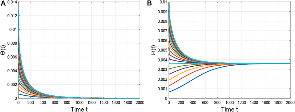
FIGURE 1. The evolution of the densities of infected edges with different initial values $S_{k0}=1-0.02\times i,\text{Θ}=0.02\times i$, $i=\mathrm{1,2},\cdots ,20.$(A) With $\beta =\mathrm{0.032.}$(B) With $\beta =\mathrm{0.033.}$

Second, we fix $\beta =0.033$ and hence ${\mathrm{ℛ}}_0=\mathrm{1.071.}$ We verify α and consider the existence and the uniqueness of the endemic equilibria. If we choose $\alpha =100$ and it is large enough, Theorem 3.7 shows that the endemic equilibrium $E^{\text{*}}$ is globally asymptotically stable. Figure 2A depicts that the densities of infected edges from differential initial data converge to an endemic equilibrium ${\text{Θ}}^{\text{*}}=0.9546$. If we pick up $\alpha =\mathrm{5,10,15,20,25},$ which are mediated values, all the trajectories of system (2) converge to their corresponding positive equilibria. From Figure 2B we find that increasing values of α gradually advances the arrival times and increases the sizes of the associated endemic equilibria. This indicates that enriching the adequate medical resources effectively reduce the risk of an infection.

FIGURE 2

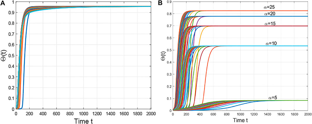
FIGURE 2. The evolution of the densities of infected edges with different initial values $S_{k0}=1-0.02\times i,{\text{Θ}}_0=0.02\times i$, $i=\mathrm{1,2},\cdots ,20.$(A) With $\alpha =100.$(B) With $\alpha =\mathrm{5,10,15,20,25.}$

Third, if we fix the structure of the network, then a key value ${\alpha }_0=\frac{\langle k\rangle \langle k^3\rangle }{{\langle k^2\rangle }^2}=4.6883$ determines whether or not a backward bifurcation happens when ${\mathrm{ℛ}}_0<1.$ If we select $\alpha =6>{\alpha }_0$ and $\beta =0.032$, then ${\mathrm{ℛ}}_0<1.$ From Lemma 3.4, system exhibits a backward bifurcation at $\left({\mathrm{ℛ}}_0,{\text{Θ}}^{\text{*}}\right)=\left(\mathrm{1,0}\right).$ From Figure 3, it follows that the trajectories of system (2) partially converge to a positive level or partially move towards to zero. However, when we take $\alpha =4<{\alpha }_0,$ however, $\widehat{{\mathrm{ℛ}}_0}=4.9308>1$ does not satisfy the conditions of Theorem 3.2. Figure 3B shows that the disease-free equilibrium $E_0$ is still asymptotically stable.

FIGURE 3

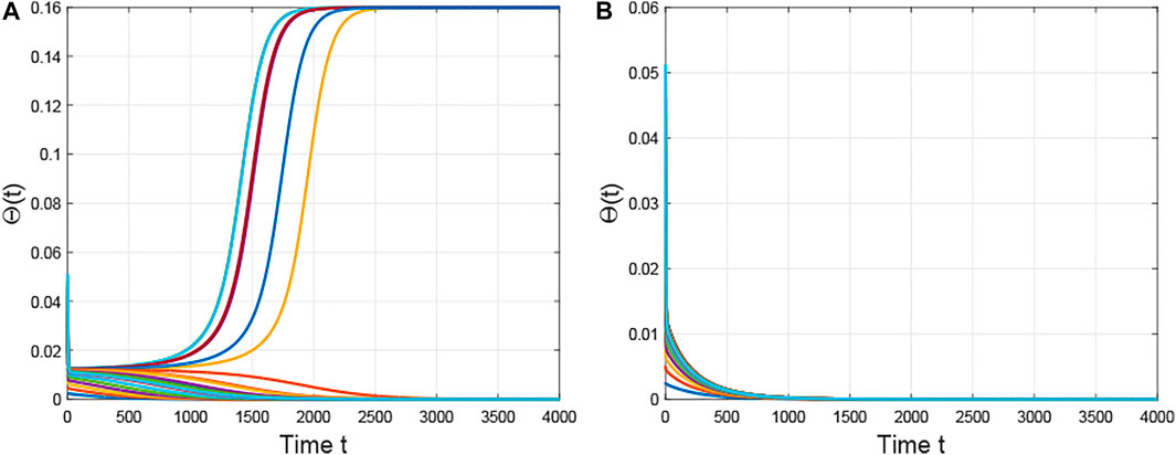
FIGURE 3. The evolution of the densities of infected edges with different initial values $S_{k0}=1-0.02\times i,{\text{Θ}}_0=0.02\times i$, $i=\mathrm{1,2},\cdots ,20.$(A) with $\alpha =6.$(B) with $\alpha =4.$

Finally, we want further insight into the existence of endemic equilibria when ${\mathrm{ℛ}}_0<1.$ We take the parameters similar to case one except α. In this case, ${\mathrm{ℛ}}_0=0.9862<1.$ As we know, the endemic ${\text{Θ}}^{\text{*}}$ is a function with respect to α and ${\mathrm{ℛ}}_0$. If we change values of α from 4.8 to 6.8 with step 0.5. Figure 4 suggests that there always exists a backward bifurcation; In addition, the lag effect α controls the depth of the backward bifurcation; the larger α, the bigger the depth of the bifurcation. α is bigger in case of strength of lag effects of medical resources. Figure 4B displays the distributions of the positive equilibria in a given region $\left({\mathrm{ℛ}}_0,\alpha \right).$ In the blue region, system (2) has only unique disease-free equilibrium $E_0$, which is globally asymptotically stable; In the grey region, a backward bifurcation occurs, i.e, system (2) exhibits a bistable phenomena, one endemic equilibria with a large value is stable and the other one with a small value is unstable; Moreover, the disease-free equilibrium $E_0$ is locally stable. In the green region, system (2) has a unique endemic equilibrium and it is stable.

FIGURE 4

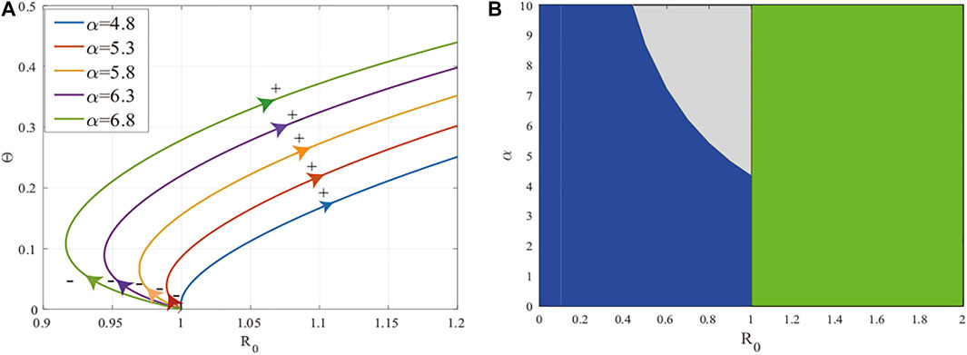
FIGURE 4. Backward bifurcation in system (2). (A) The figure of function $\text{Θ}$ associated with ${\mathrm{ℛ}}_0$ with different values of $\alpha .$(B) The diagram of bifurcation phase on the $\left({\mathrm{ℛ}}_0,\alpha \right)-$ plane.

5 Discussion

In this paper, we considered a mean-field degree-based SIS epidemic model with a saturated treatment function. First, we adopted an edge-compartmental approach to simplify a pure degree-based model to a degree-edge-mixed model. Second, we proposed a novel method-a geometric approach to completely study the stability of each feasible equilibrium. The proposed model exhibits a backward bifurcation, i.e, ${\mathrm{ℛ}}_0<1$ does not sufficiently guarantee the eradication of an outbreak.

Compared with the results in [5, 25], a degree-based SIS epidemic model on complex networks shows a threshold dynamic, in the sense that, if ${\mathrm{ℛ}}_0<1,$ then the disease-free equilibrium $E_0$ is globally asymptotically stable; Otherwise, the unique endemic equilibrium $E^{\text{*}}$ is globally asymptotically stable. However, in our system, a saturated treatment function radically altered such a threshold property. Lemma 3.4 suggests that the hysteretic effect leads to the occurrence of backward bifurcation.

The basic reproduction number ${\mathrm{ℛ}}_0$ has no relationship with the lag effect of α. However, it is a vital value which determines whether or not a backward bifurcation occurs. In view of most existing results about that phenomena, they usually showed the existence and did not point out the stability of each equilibrium except some simple models with lower dimensions [2, 3, 18, 19]. In this paper, we proposed a geometric approach to completely solve such an issue. Our results suggest that whereas ${\mathrm{ℛ}}_0<1$ and $\alpha >\frac{\langle k\rangle \langle k^3\rangle }{{\langle k^2\rangle }^2}$, one positive equilibrium with a larger value is stable; the other with small data is unstable. Their stabilities definitely depend on those signs of tangent slopes of the epidemic curve $F\left(\text{Θ}\right).$ To establish it, we build a bridge between the local stability and the derivative of the epidemic curve, which is a universal result for any system even if it has a more complex structure [23].

Generally, the contact magnitude of an outbreak is characterized by the average degree $\langle k\rangle$ and its heterogeneity is measured by the two movement degrees $\langle k^2\rangle$ of a network. To assess how the heterogeneity of a network affects the transmission of an infection, we fixed all the parameters as in part one of Section 4. Then we take the degree distribution function $p\left(k\right)=k^{-r}$ with $r=-2.49,-2.5,-2.505,$ respectively. Then $\langle k\rangle =1.840,1.7995$ and 1.7924. As $\langle k\rangle$ increases, the system undergoes three different phenomena: the extinction of an outbreak, the occurrence of a backward bifurcation, and the persistence of the disease (see Figure 5). This expounds that the system (2) undergoes a phase transition with the change of the network structure.

FIGURE 5

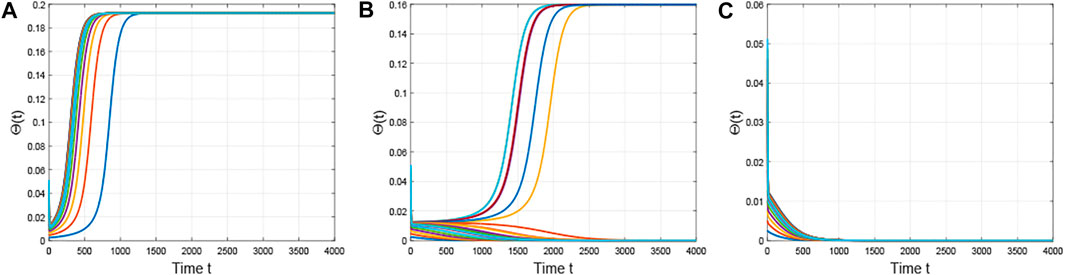
FIGURE 5. Time series of the densities of $\text{Θ}$ with different degree distributions. (A) With $\langle k\rangle =\mathrm{1.840.}$(B) With $\langle k\rangle =1.7995$(C) With $\langle k\rangle =1.7924$.

From an epidemiological viewpoint, the occurrence of a backward bifurcation implies that those control measures enabling ${\mathrm{ℛ}}_0<1$ do not efficiently ensures the eradication of an infection. In this case, the evolution of the disease heavily depends on the initial numbers of infected individuals. If it is small, the disease will die out; Otherwise, it will maintain a positive level and it cannot be radically eradicated from a region or a county. Hence, enhancing the management and allocations of medical resources plays an important role in slowing down a disease prevalence. Those control measures are in favor of effectively reducing the lag effect due to the limitations of medical resources as long as people face an emerging disease.

However, there are some limitations of this paper. First, we do not incorporate the population demography into the modeling process because introducing birth and death nodes essentially changes the topology of a network [27, 28]. This makes the model become too complex and then it has been become an unresolved issue to analyze its dynamical behaviors from mathematical view of points. Second, we do not couple individual contact data with some reported data for a realistic disease to study its evolutionary behaviors [29]. Third, we do not consider the convolution of information spread and epidemic transmission on multi-layered networks [30]. To carry out such a project, it may provide some valuable control suggestions for policymakers and public health government. We leave these for our future works.

Data Availability Statement

The original contributions presented in the study are included in the article/Supplementary Material, further inquiries can be directed to the corresponding author.

Author Contributions

JY and XW conceived of the presented idea. JY developed the theory and performed the computations. XW verified the analytical methods. All authors discussed the results and contributed to the final manuscript. JY designed the modeling process and analyzed theoretical results. XW conceived of the study and helped to draft the manuscript. All the authors read and approved the final manuscript.

Funding

This work is partially supported by the National Natural Science Foundation of China (No.12001339, No.61573016), and the Shanxi Province Science Foundation for Youths (No. 201901D211413). Shanxi University of Finance and Economics Youth Research Fund Project (QN-2019017).

Conflict of Interest

The authors declare that the research was conducted in the absence of any commercial or financial relationships that could be construed as a potential conflict of interest.

References

1. Kermack W, McKendrick A. A Contribution to the Mathematical Theory of Epidemics. Proc R Soc Lond A (1927) 115:700–21. doi:10.1098/rspa.1927.0118

CrossRef Full Text | Google Scholar

2. van den Driessche P, Watmough J. A Simple Sis Epidemic Model with a Backward Bifurcation. J Math Biol (2000) 40:525–40. doi:10.1007/s002850000032

PubMed Abstract | CrossRef Full Text | Google Scholar

3. Kribs-Zaleta CM, Velasco-Hernández JX. A Simple Vaccination Model with Multiple Endemic States. Math Biosciences (2000) 164:183–201. doi:10.1016/s0025-5564(00)00003-1

CrossRef Full Text | Google Scholar

4. Wang L, Dai G-z. Global Stability of Virus Spreading in Complex Heterogeneous Networks. SIAM J Appl Math (2008) 68:1495–502. doi:10.1137/070694582

CrossRef Full Text | Google Scholar

5. d’Onofrio A. A Note on the Global Behaviour of the Network-Based Sis Epidemic Model. Nonlinear Anal Real World Appl (2008) 9:1567–72. doi:10.1016/j.nonrwa.2007.04.001

CrossRef Full Text | Google Scholar

6. Zhu L, Guan G, Li Y. Nonlinear Dynamical Analysis and Control Strategies of a Network-Based Sis Epidemic Model with Time Delay. Appl Math Model (2019) 70:512–31. doi:10.1016/j.apm.2019.01.037

CrossRef Full Text | Google Scholar

7. Xie Y, Wang Z, Lu J, Li Y. Stability Analysis and Control Strategies for a New Sis Epidemic Model in Heterogeneous Networks. Appl Math Comput (2020) 383:125381. doi:10.1016/j.amc.2020.125381

CrossRef Full Text | Google Scholar

8. Lau MSY, Dalziel BD, Funk S, McClelland A, Tiffany A, Riley S, et al. Spatial and Temporal Dynamics of Superspreading Events in the 2014-2015 West Africa Ebola Epidemic. Proc Natl Acad Sci USA (2017) 114:2337–42. doi:10.1073/pnas.1614595114

PubMed Abstract | CrossRef Full Text | Google Scholar

9. Pastor-Satorras R, Vespignani A. Epidemic Spreading in Scale-free Networks. Phys Rev Lett (2001) 86:3200–3. doi:10.1103/physrevlett.86.3200

PubMed Abstract | CrossRef Full Text | Google Scholar

10. Wang X, Yang J. Dynamical Analysis of a Mean-Field Vector-Borne Diseases Model on Complex Networks: An Edge Based Compartmental Approach. Chaos (2008) 30:013103. doi:10.1063/1.5116209

PubMed Abstract | CrossRef Full Text | Google Scholar

11. Wang Y, Jin Z, Yang Z, Zhang Z-K, Zhou T, Sun G-Q. Global Analysis of an Sis Model with an Infective Vector on Complex Networks. Nonlinear Anal Real World Appl (2012) 13:543–57. doi:10.1016/j.nonrwa.2011.07.033

CrossRef Full Text | Google Scholar

12. Yang M, Chen G, Fu X. A Modified Sis Model with an Infective Medium on Complex Networks and its Global Stability. Physica A: Stat Mech its Appl (2011) 390:2408–13. doi:10.1016/j.physa.2011.02.007

CrossRef Full Text | Google Scholar

13. Wu Q, Fu X, Small M, Xu X-J. The Impact of Awareness on Epidemic Spreading in Networks. Chaos (2012) 22:013101. doi:10.1063/1.3673573

PubMed Abstract | CrossRef Full Text | Google Scholar

14. Yang J, Kuniya T, Luo X. Competitive Exclusion in a Multi-Strain Sis Epidemic Model on Complex Networks. Electron J Differ Equat (2019) 2019:1–30.

Google Scholar

15. van den Driessche P, Watmough J. Reproduction Numbers and Sub-threshold Endemic Equilibria for Compartmental Models of Disease Transmission. Math Biosciences (2002) 180:29–48. doi:10.1016/s0025-5564(02)00108-6

CrossRef Full Text | Google Scholar

16. Keeling MJ, Grenfell BT. Individual-based Perspectives on R0. J Theor Biol (2000) 203:51–61. doi:10.1006/jtbi.1999.1064

PubMed Abstract | CrossRef Full Text | Google Scholar

17. Diekmann O, Heesterbeek JA, Metz JA. On the Definition and the Computation of the Basic Reproduction Ratio R0 in Models for Infectious Diseases in Heterogeneous Populations. J Math Biol (1990) 28:365–82. doi:10.1007/BF00178324

PubMed Abstract | CrossRef Full Text | Google Scholar

18. Wang W. Backward Bifurcation of an Epidemic Model with Treatment. Math Biosciences (2006) 201:58–71. doi:10.1016/j.mbs.2005.12.022

PubMed Abstract | CrossRef Full Text | Google Scholar

19. Cui J, Mu X, Wan H. Saturation Recovery Leads to Multiple Endemic Equilibria and Backward Bifurcation. J Theor Biol (2008) 254:275–83. doi:10.1016/j.jtbi.2008.05.015

PubMed Abstract | CrossRef Full Text | Google Scholar

20. Buonomo B, Lacitignola D. On the Backward Bifurcation of a Vaccination Model with Nonlinear Incidence. Namc (2011) 16:30–46. doi:10.15388/na.16.1.14113

CrossRef Full Text | Google Scholar

21. Garba SM, Gumel AB, Abu Bakar MR. Backward Bifurcations in Dengue Transmission Dynamics. Math Biosciences (2008) 215:11–25. doi:10.1016/j.mbs.2008.05.002

PubMed Abstract | CrossRef Full Text | Google Scholar

22. Gumel AB. Causes of Backward Bifurcations in Some Epidemiological Models. J Math Anal Appl (2012) 395:355–65. doi:10.1016/j.jmaa.2012.04.077

CrossRef Full Text | Google Scholar

23. Li C-H, Yousef AM. Bifurcation Analysis of a Network-Based Sir Epidemic Model with Saturated Treatment Function. Chaos (2019) 29:033129. doi:10.1063/1.5079631

PubMed Abstract | CrossRef Full Text | Google Scholar

24. Huang Y-J, Li C-H. Backward Bifurcation and Stability Analysis of a Network-Based Sis Epidemic Model with Saturated Treatment Function. Physica A: Stat Mech its Appl (2019) 527:121407. doi:10.1016/j.physa.2019.121407

CrossRef Full Text | Google Scholar

25. Yang J, Xu F. The Computational Approach for the Basic Reproduction Number of Epidemic Models on Complex Networks. IEEE Access (2019) 7:26474–9. doi:10.1109/access.2019.2898639

CrossRef Full Text | Google Scholar

26. Martcheva M. Methods for Deriving Necessary and Sufficient Conditions for Backward Bifurcation. J Biol Dyn (2019) 13:538–66. doi:10.1080/17513758.2019.1647359

PubMed Abstract | CrossRef Full Text | Google Scholar

27. Jin Z, Sun G, Sun G, Zhu H. Epidemic Models for Complex Networks with Demographics. Math Biosci Engin (2014) 11:1295–317. doi:10.3934/mbe.2014.11.1295

CrossRef Full Text | Google Scholar

28. Yin Q, Wang Z, Xia C, Dehmer M, Emmert-Streib F, Jin Z. A Novel Epidemic Model Considering Demographics and Intercity Commuting on Complex Dynamical Networks. Appl Math Comput (2020) 386:125517. doi:10.1016/j.amc.2020.125517

CrossRef Full Text | Google Scholar

29. Yang J, Wang G, Wang G, Zhang S. Impact of Household Quarantine on SARS-Cov-2 Infection in mainland China: A Mean-Field Modelling Approach. Math Biosci Engin (2020) 17:4500–12. doi:10.3934/mbe.2020248

PubMed Abstract | CrossRef Full Text | Google Scholar

30. Wang Z, Xia C. Co-evolution Spreading of Multiple Information and Epidemics on Two-Layered Networks under the Influence of Mass media. Nonlinear Dyn (2020) 102:3039–52. doi:10.1007/s11071-020-06021-7

CrossRef Full Text | Google Scholar