Using a Heliospheric Upwinding eXtrapolation Technique to Magnetically Connect Different Regions of the Heliosphere

Understanding how coronal structure propagates and evolves from the Sun and into the heliosphere has been thoroughly explored using sophisticated MHD models. From these, we have a reasonably good working understanding of the dynamical processes that shape the formation and evolution of stream interaction regions and rarefactions, including their locations, orientations, and structure. However, given the technical expertize required to produce, maintain, and run global MHD models, their use has been relatively restricted. In this study, we refine a simple Heliospheric eXtrapolation Technique (HUX) to include not only forward mapping from the Sun to 1 AU (or elsewhere), but backward mapping toward the Sun. We demonstrate that this technique can provide substantially more accurate mappings than the standard, and often applied “ballistic” approximation. We also use machine learning (ML) methods to explore whether the HUX approximation to the momentum equation can be refined without loss of simplicity, finding that it likely provides the optimum balance. We suggest that HUX can be used, in conjunction with coronal models (PFSS or MHD) to more accurately connect measurements made at 1 AU, Stereo-A, Parker Solar Probe, and Solar Orbiter with their solar sources. In particular, the HUX technique: 1) provides a substantial improvement over the “ballistic” approximation for connecting to the source longitude of streams; 2) is almost as accurate, but considerably easier to implement than MHD models; and 3) can be applied as a general tool to magnetically connect different regions of the inner heliosphere together, as well as providing a simple 3-D reconstruction.

1 Introduction

Plasma is heated in the corona and accelerates away from it to form the solar wind. It is convenient (although probably an oversimplification) to separate what we believe to be intrinsically spatial variations from temporal variations [1]. The former is the repeating large-scale structure we observe in the interplanetary medium from one rotation to the next, while the latter manifests as sporadic eruptions of transient phenomena, including coronal mass ejections (CMEs) as well a rich set of other effects, such as jets, plumes, small-scale flux ropes, etc., We recognize, however, that even the structure we label as “spatial”, is undoubtedly driven, at least to some extent, by time-dependent phenomena. Nevertheless, it remains useful to treat the large-scale, quasi-corotating structure as a predominantly time-stationary process. This is supported by many observations over the last 50+ years, which show that, particularly during the declining phase of the solar activity cycle, and the interval surrounding solar minimum, in particular, global models relying on steady-state solutions can capture the essential features of solar wind streams (e.g., [2–4]).

Being able to connect in situ measurements back to their solar sources, or explore the evolution of plasma as it propagates away from the Sun is both scientifically and operationally important. For example, the source of the slow solar wind remains the topic of considerable debate; thus, being able to estimate from which regions on the Sun specific plasma came from could shed light on its origin (e.g., [5]). Operationally, both ambient solar wind and empirically based coronal mass ejections (CMEs) can be mapped from the Sun to the Earth to improve space weather forecasts (e.g., [6]). Over the years, a number of techniques have been developed to map solar wind plasma from one point in the solar wind to another. The simplest is the so-called “ballistic” approximation [7], which assumes that parcels of plasma travel radially, and maintain a constant speed as they propagate from one location to another (either inwards or outwards). The technique is simple to implement, but can lead to substantial errors, particularly at compression regions, where the interaction between plasma of different speeds is dynamic. Sophisticated global MHD models (e.g., [8], address these limitations by providing three-dimensional dynamic evolution of the plasma. However, they are difficult to develop and require significant resources to run them.

[9]; herein referred to as Paper 1, introduced the concept of Heliospheric Upwinding eXtrapolation (HUX). This simplified method bridged the gap between kinematic (i.e., constant speed) mapping (e.g., [7]) and full MHD calculations (e.g., [2]), providing a surprisingly accurate extrapolation of solar wind speeds close to the Sun to 1 AU or beyond. By neglecting the pressure gradient and gravity terms, they were able to show that the momentum equation reduced to the inviscid Burger’s equation, which could be easily converted to a difference algorithm and used to evolve speed profiles near the Sun radially outwards. Additionally, to account for the general acceleration of the solar wind near the Sun, a simple expression was derived and applied. Together, these two components allowed MHD solutions to be reproduced with high accuracy (Pearson correlation coefficient, $CC\sim 0.98$).

Several studies have leveraged the HUX technique to improve space weather forecasts of solar wind streams. [6]; for example, developed ensemble solutions of solar wind conditions at Earth by sampling a range of latitudes about the sub-Earth point, resulting in more accurate forecasts and variances that accurately captured the model uncertainty [10]. used HUX to propagate several competing models for defining the speed of the solar wind in the high corona out to 1 AU, allowing them to assess forecasting performance among them. They also found that the ability to incorporate multiple realizations (which would not have been computationally feasible with global MHD model solutions), they were able to improve forecasting performance of all the models considered. More recently [11], refined HUX by generalizing it to a form similar to that of the viscous Burger’s equation (Tunable HUX, or THUX), essentially adding an additional term to mimic the effects of viscosity. It is worth noting that this also introduced a new free parameter, η, that can be tuned to make the model comparisons better, and, the changes in the forecasted speeds were found to be modest, and not obviously improvements (see their Figure 1) [12]. combined the HUX approach with a machine learning (ML) algorithm (specifically, Gradient Boosting Regressors), to produce a fast and accurate model for forecasting ambient solar wind conditions at Earth.

The HUX technique is also being incorporated into space weather programs. [13]; for example, have integrated HUX into a pilot program for developing space weather capabilities for the Indian Space Research Organization (ISRO). Additionally [14], have used HUX within an ensemble-based CME arrival prediction model (ELEvoHI), finding that the combination of the WSA model for prescribing the speed at the inner boundary and HUX resulted in a reduction in the Mean Absolute Error (MAE) by almost 2 h, in comparison to other techniques using the observed solar wind speed at L1.

The HUX technique has also been generalized to study time-dependent phenomena [15]. interpreted the $\partial /\partial t$ term not in terms of longitude, but explicitly as time, to allow them to consider both time-stationary evolution as well as direct temporal evolution, such as the propagation of simple “pulse-like” ICME structures. The so-called HUXt generalization was shown to produce results in the equatorial plane that were comparable to 3D global MHD solutions, but at a tiny fraction of the computational resources, positioning it to be a useful, complementary tool for generating ensemble-based forecasts.

In this study, we describe a simple refinement to the HUX allowing the user to map solar wind streams from 1 AU (or elsewhere) back to the Sun, which can have a substantial impact on the inferred source longitudes of the observed plasma. Additionally, using a data-driven sparse regression method, we explore whether there are any simple improvements that can be applied to the HUX approach. Finally, we explore the possible impacts of including differential rotation, as well as any constraints imposed by resolution.

2 Models

Here, we introduce the three main modeling techniques that are applied in our study. Specifically: 1) ballistic mapping; 2) MHD modeling; and 3) the HUX technique.

2.1 Ballistic Mapping

The simplest (but least useful) approximation we could make for evolving the speed of the solar wind as it propagates away from the Sun is to assume that it does not change speed in response to dynamical interactions between adjacent parcels of plasma. This has a number of obvious problems, perhaps largest of which is that in mapping the speeds out, it becomes possible for faster parcels to outrun slower ones. By virtue of the fact that the solar wind can be reasonably approximated as a fluid, this is patently nonphysical. When the procedure is instead applied in the reverse direction, this can lead to the well known problems of “dwells”, where parcels of plasma observed at a later times in the solar wind map back to earlier launch times at the Sun, again by apparently “crossing paths” [16].

In spite of its simplicity, for completeness, we formally define the ballistic approximation as:

$v_{i+1,j}=v_{i,j}(1)$

which simply states that the speed at $i+1$ is the same as the speed at i, where i is the radial index and j is the azimuthal or longitudinal index. In terms of mapping solar wind streams from one location to another, and usually back to the Sun from 1 AU, this allows us to estimate the change in longitude as follows:

$\text{Δ}\varphi =-{\text{Ω}}_{rot}\frac{\text{Δ}r}{v_i}(2)$

where $\text{Δ}r$ is the total radial distance along which the plasma is mapped and ${\Omega }_{rot}$ is the angular frequency of the Sun’s rotation, equal to $2\pi /25.38$ days at the solar equator.

2.2 Magnetohydrodynamic Model

For our numerical experiments, we use the Magnetohydrodynamic Algorithm outside a Sphere (MAS) code, which solves the time-dependent resistive magnetohydrodynamic (MHD) equations (e.g., [8]). Although the model can be run with a range of increasingly complex energy transport processes, for the purposes of our study, we rely on either polytropic or thermodynamic solutions [4]. The inner boundary of the calculation is set to $R=30R_S$, by which point, all flow is super-Alfvénic. The outer boundary is set to 1 AU. The results presented here were undertaken with a relatively modest resolution of $281\times 181\times 361$ points in radius (r), colatitude (θ), and azimuth (ϕ), respectively; however, the analyses were performed at both higher and lower resolution without any substantial differences in the results. Although MAS is a time-dependent code, capable of modeling CMEs (e.g., [17]), in this study, we drove the model with a synoptic map of the photospheric magnetic field, allowing it to evolve in time until it reached a steady-state equilibrium [2]. We focus on Carrington Rotation (CR) 2068, which was a generally quiescent time period, but also representative of the declining phase of the solar cycle, with two strong high-speed streams per rotation. Thus, it is ideal for exploring the evolution of large-scale structure in the solar wind. However, we also analyzed a number of other periods (e.g., CRs 2050, 2068, 2100, 2170, and 2231) to verify that the results held in general. Please see the GitHub repository supporting this study for more examples (https://github.com/predsci/HUX).

2.3 Heliospheric Upwinding eXtrapolation Technique

In an earlier study [9], herein referred to as paper 1, we developed a simple mapping technique that approaches the simplicity of the ballistic approach but retains most of the accuracy of the MHD approach, by reducing the momentum equation to the much simpler Burger equation.

Briefly, the solar wind motion can be described as the fluid momentum equation in a corotating frame of reference:

$-{\text{Ω}}_{\mathit{rot}}\frac{\partial \mathbf{v}}{\partial \varphi }+\left(\mathbf{v}\cdot \partial \right)\mathbf{v}=\frac{1}{\rho }\nabla P-\frac{G{M}_S}{r^2}{\mathrm{e}}_{\mathrm{r}}(3)$

where ρ is the proton mass density, V is the velocity, p is the thermal pressure, G is the gravitational constant, M_s is the mass of the Sun, and γ is the polytropic index. This contrasts the more common form of the momentum equation in that the time derivative, $\partial /\partial t$, has been replaced by the term $-{\text{Ω}}_{rot}\partial /\partial \varphi$, which is exact for time-stationary flows in a corotating frame of reference. By neglecting magnetic field, pressure gradient and gravity, the fluid momentum equation reduces to the inviscid Burgers’ equation:

$\frac{\partial v_r}{\partial \varphi }=\frac{1}{{\text{Ω}}_{rot}}{v}_r\frac{\partial v_r}{\partial r}(4)$

Using the forward upwind difference algorithm, we can represent this as:

$v_{i+1,j}=v_{i,j}+\frac{\text{Δ}r{\text{Ω}}_{rot}}{v_{i,j}}\left(\frac{v_{i,j+1}-v_{i,j}}{\text{Δ}\varphi }\right)(5)$

Equation 5, thus, allows us to take a set of velocity measurements at some radius, i, as a function of longitude (j), and march them forward to larger heliocentric distances. We denote this operation as HUX-forward, or HUX-f. It is straightforward to show that given a set of measurements at some radius, i, we can march them back to the Sun with the following expression:

$v_{i-1,j}=v_{i,j}+\frac{\text{Δ}r{\text{Ω}}_{rot}}{v_{i,j}}\left(\frac{v_{i,j-1}-v_{i,j}}{\text{Δ}\varphi }\right)(6)$

We denote this form as HUX-backward, or HUX-b.

As discussed in more detail in paper 1, we can apply an acceleration term to the forward mapped speeds of the form:

$v_{acc}\left(r\right)=\alpha v_{ro}\left(1-\text{exp}\left(-r/r_h\right)\right),(7)$

where $v_{ro}$ is the speed at the inner boundary $\left(r_o\right)$, α is some factor by which the initial speed is increases, and $r_h$ is the scale length over which the acceleration spans. Thus, the final speed is enhanced as follows:

$v_f\left(r\right)=v_0+v_{acc}\left(r\right)(8)$

Similarly, by inspection, we can define a deceleration term for the HUX-b mapping as follows:

$v_b\left(r\right)=v_0-v_{acc}\left(r\right)(9)$

3 Results

3.1 A “Ground Truth” From the Magnetohydrodynamic Results and Comparison With the Ballistic Approximation

As in paper 1, we use a global MHD solution as the “ground truth” for validating the more approximate HUX results. We focus again on CR 2068, but also add a number of other Carrington rotations to the analysis, to ensure that we do not over-generalize the results from one solution. In Figure 2A we summarize the equatorial magnetic field lines from CR 2068. In contrast to the usual way that field lines are drawn by tracing along the magnetic field vectors, in this case, we use the velocity field directly to evolve the field lines since they are convected out along the plasma flow, and there are no time-dependent effects to complicate matters. Thus, strictly speaking, these “field lines” are really streamlines. They are arbitrarily colored, but, importantly, each source longitude is drawn with the same color in subsequent plots, allowing us to directly compare the relative evolution of the “field lines” between approaches.

FIGURE 1

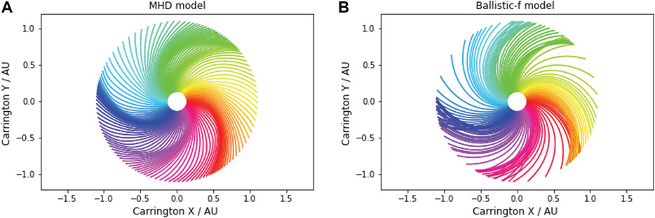
FIGURE 1. (A) Field lines traced out from the inner boundary of the MHD solution using the MHD velocity solution. (B) Field lines traced out from the inner equatorial boundary assuming that the speed for that field line remains the same (i.e., the ballistic approximation).

FIGURE 2

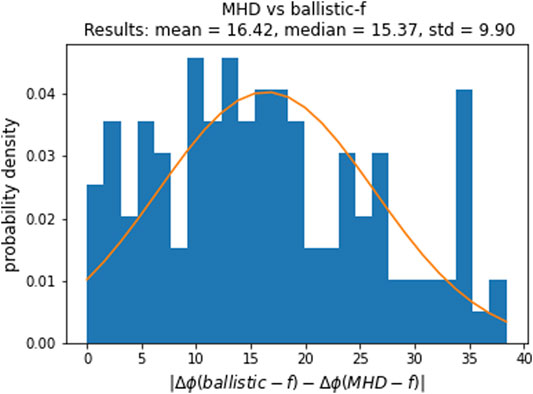
FIGURE 2. Probability density (histogram) of the difference between the ballistically mapped longitudes and the MHD-mapped longitudes of the field lines from the inner boundary at 30R_s to 1 AU. The blue blocks show the actual frequency while the orange curve provides a Gaussian fit to the data. The Gaussian fit is used only as a practical way to estimate the spread in the values, and not to suggest that the errors are normally distributed.

In Figure 2B we have drawn field lines from the same sources under the assumption that the speed does not evolve as the field is dragged radially out with the flow. This is the so-called ballistic approximation. We note that while field lines generally terminate near the correct location, there is considerable variability in the accuracy of the mapping. More importantly, we see that the “field lines” overlap one another; a physically forbidden result.

To more quantitatively assess the difference between the MHD mapping and the ballistic mapping, in Figure 1, we show the difference between the ballistically mapped longitudes and the MHD-mapped longitudes of the field lines. The orange curve is a Gaussian fit to the data to enable an estimate of the statistical parameters for the distribution of errors. We find that the mean/median error in the ballistic mapping is ${16.42/15.37}^{\circ }$, with a SD of ${9.9}^{\circ }$. Thus, even under the absolutely quietest of conditions, we can expect errors in mapping the source longitudes from the Sun to 1 AU of at least ${15}^{\circ }$. Moreover, this assumes that we know what was the initial speed of the plasma dragging the field out. When that must be assumed, say, 400 km/s⁻¹, the errors would be substantially larger. It should be noted, however, that when mapping out to different radial distances, the associated errors would be proportional to the distance mapped. Between, Solar Orbiter and Parker Solar Probe (PSP), for example, when separated by fractions of an AU, the errors may be considerably smaller.

3.2 Mapping Solar Wind Streams Out From the Sun With HUX-f

Figure 3 (top panel) shows the radial speed at the inner boundary of the MHD calculation ($30R_S$). This profile shows a typical structure for the declining phase of the solar cycle, with slow flow organized about the equator, and including the presence of an equatorial coronal hole centred at approximately ${100}^{\circ }$. The undulation of the slow-flow band about the heliographic equator reflects the fact that the wind structure is organized about the heliomagnetic equator, and that a tilted dipole field component dominates during this period. The equatorial coronal hole also underscores the presence of pseudo-streamer structure during this time [18]. As this wind propagates into the heliosphere and the Sun rotates underneath it, the corotating sources move westward; thus, by 1 AU even in the absence of dynamical evolution, the global pattern appears to have precessed to earlier Carrington longitudes (middle panel). Dynamical evolution, however, also modifies the picture such that where fast wind lies to the east of slower wind, it is compressed, whereas where fast wind lies to the west of slower wind, a rarefaction is created. These features are, to a large extent, captured by the HUX-f procedure (bottom panel). Although there are some quantitative differences between the MHD and HUX-f solutions, overall, the main inference is positive: The HUX-f technique has captured the evolution of the streams. To investigate this in more detail, we can extract slices at specific latitudes, which would correspond to time series under the assumption that the structure at the Sun is not changing in time.

FIGURE 3

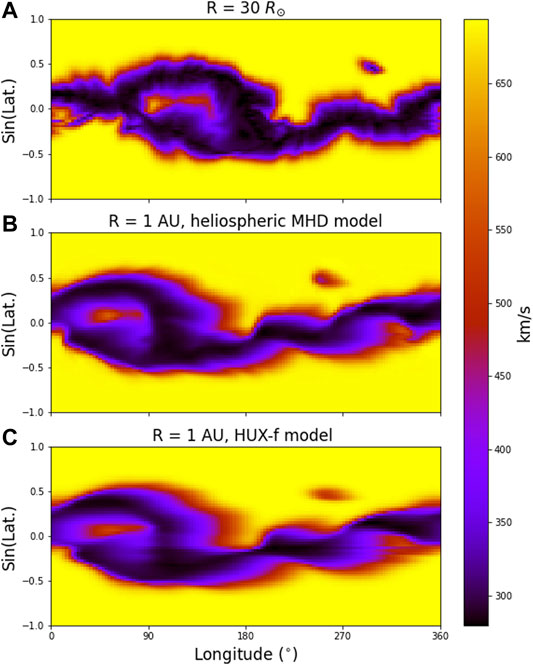
FIGURE 3. (A) Solar wind radial speed as a function of Carrington longitude and sin (latitude) at the inner boundary of the MHD simulation. (B) solar wind speed at 1 AU as computed by the MHD solution. (C) Solar wind speed at 1 AU as estimated using the HUX-f technique.

Before doing this, however, it is useful to assess how much evolution has taken place from the inner radial boundary to 1 AU in the MHD model. In Figure 4A, we compare the equatorial solar wind at $30R_S$ (red) against the final speed at 1 AU. Clearly, the streams have evolved substantially in moving from the inner to the outer boundary. Much of this evolution is intuitively easy to understand. First, there is a general progression to early longitudes (eastward) due to the fact that the Sun and hence source of a particular high-speed stream is moving westward. Second, there is a general acceleration of all plasma. Third, the western edge of each stream tends to steepen (this is the compression side of the stream), while the eastern edge broadens, as an expansion wave propagates into the wind ahead and behind (e.g., [19]). In Figure 4B we compare the same 1 AU MHD result with the HUX-f-mapped stream. As described in paper 1 in more detail, this simple method has captured a significant fraction of the aforementioned evolution (CC = 0.96). The most noteworthy discrepancy is that it underestimates the peak values and overestimates the troughs.

FIGURE 4

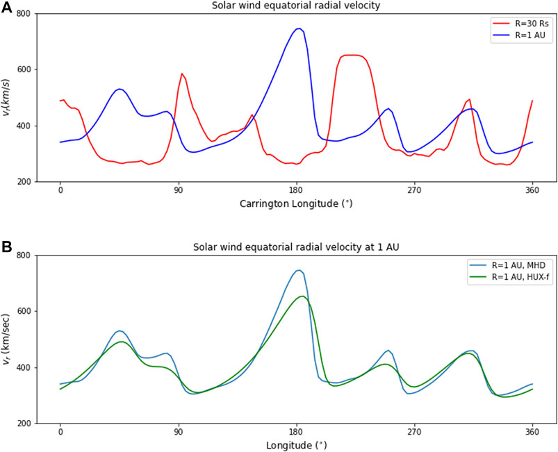
FIGURE 4. (A) Comparison of solar wind speed at the equator at 30 solar radii (blue) and 1 AU (red) from MHD solution. (B) Comparison of solar speed at the equator at 1 AU from the MHD solution (blue) and HUX-f technique (green).

We explore the errors more quantitatively in Figure 5, which shows the difference between the HUX-f and MHD speeds, normalized to the MHD speeds at 1 AU. On average, the errors associated with the HUX-f approach are 0.086, or approximately 9%. Comparison with Figure 3 also suggests that the sense of the errors are systematic, with positive errors associated with compression regions, and negative errors associated with rarefactions. This is reinforced qualitatively in Figure 4, which, as already noted, showed that the HUX-f technique underestimates the peak of the high-speed streams, but also tends to overestimate the troughs. Nevertheless, the key point is that the average errors are substantially smaller than, say, a ballistic approximation would produce.

FIGURE 5

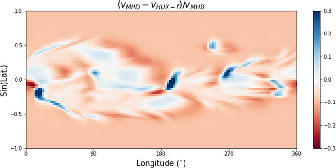
FIGURE 5. Estimate of the error in the HUX-f mapping as compared to the MHD result at 1 AU. Positive errors are shown in blue, negative errors are red, and an exact match appears as white.

As a final consideration of the errors associated with the mapped speeds, in Figure 6A we show the point-by-point relationship between all grid points (i.e., all latitudes and longitudes) at 1 AU for the HUX-f and MHD solutions. The computed Pearson correlation coefficient for this was found to be 0.997. However, it should be noted that this is likely heavily biased by the large fraction of the solar wind volume that is not undergoing any significant evolution, that is, the fastest and slowest wind pinning the extremes of the correlation. A more appropriate estimate is to limit the comparison to the equator. This is accomplished in Figure 6B, where the equatorial values as well as one slice on either side have been plotted. The correlation coefficient for this subset, while still remarkably high (0.96) is lower than for the full comparison.

FIGURE 6

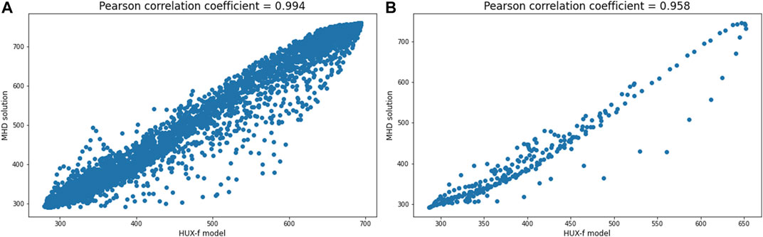
FIGURE 6. Point by point scatter plot between MHD and HUX-f results. (A) For all latitudes, the Pearson correlation coefficient (PCC) was 0.994. (B) For a narrow band about the heliographic equator, the PCC was 0.958.

3.3 Outward Extrapolation of Field Lines Using HUX-f

We can also map out field lines using the HUX-f technique and compare them with the MHD results. In Figure 7B we have drawn field lines from the same sources as in Figure 1. At least qualitatively, comparison between panels (a) and (b) suggests a very close match between the MHD and HUX-f approaches.

FIGURE 7

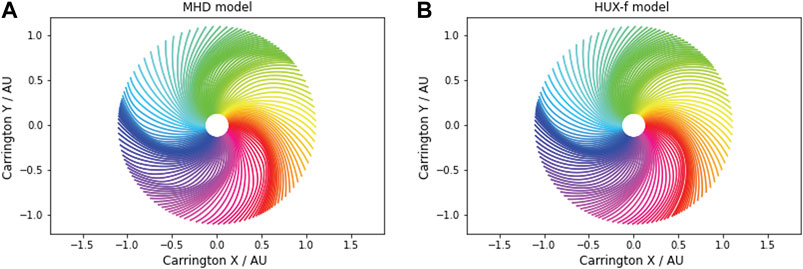
FIGURE 7. (A) Field lines traced out from the inner boundary of the MHD solution using the MHD velocity solution. (B) Field lines traced out from the inner equatorial boundary assuming that the speed for that field line remains the same.

Again, to more quantitatively assess the difference between the MHD mapping and the HUX-f mapping, in Figure 8, we show the difference between the HUX-f-mapped longitudes and the MHD-mapped longitudes of the field lines. This time, we find that the mean/median error in the ballistic mapping is $1.14/{1.00}^{\circ }$, with a SD of ${0.82}^{\circ }$. These values are a factor of 15 or more smaller than the errors associated with the ballistic mapping. Thus, given accurate values of solar wind speed, we can map them out with an accuracy of $\sim 1^{\circ }$.

FIGURE 8

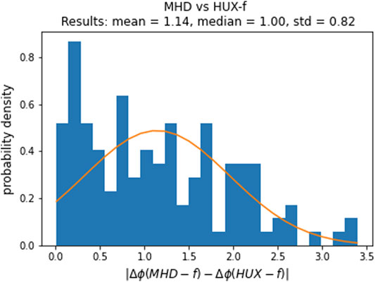
FIGURE 8. Probability density (histogram) of difference between the ballistically mapped longitudes and the MHD-mapped longitudes of the field lines. The blue blocks show the actual frequency while the orange curve provides a Gaussian fit to these data.

3.4 Inward Extrapolation of Field Lines Using Heliospheric Upwinding eXtrapolation-B

Finally, we can repeat the analysis using the HUX-b technique. In this case, we start the mapping at 1 AU and draw the field lines back to the Sun. In Figure 9B we have drawn field lines from the same MHD sources at 1 AU using the HUX-b formulation. Again, at least qualitatively, comparison between panels (a) and (b) suggest a close match between the MHD and HUX-b approaches. However, it can be noted that in the high-speed streams (where the field lines are more radial and show more space between them), the HUX-b field lines are not separated to the same degree. Additionally, where the field lines are closer together, the effect is reduced in the HUX-b solution. We can interpret this in terms of compression and rarefaction regions, suggesting that the HUX-b solutions would produce weaker compression regions and less tenuous rarefaction regions that would, in reality, be present. Nevertheless, a novel application of such a visualization is that it allows one to infer the location of compression/rarefaction regions with only a knowledge of the velocity field.

FIGURE 9

FIGURE 9. (A) Field lines traced out from the inner boundary of the of the MHD solution using the MHD velocity solution. (B) Field lines traced out from the inner equatorial boundary assuming that the speed for that field line remains the same.

Considering the distribution in the errors, in Figure 10, we show the difference between the HUX-b-mapped longitudes and the MHD-b-mapped longitudes of the field lines. This time, we find that the mean/median error in the ballistic mapping is $2.64/{2.36}^{\circ }$, with a standard deviation (s.d.) of ${1.67}^{\circ }$. These values are a factor of seven smaller than the errors associated with the ballistic mapping. Thus, even though they are larger than the HUX-f results, they are significantly less than the ballistic mapping.

FIGURE 10

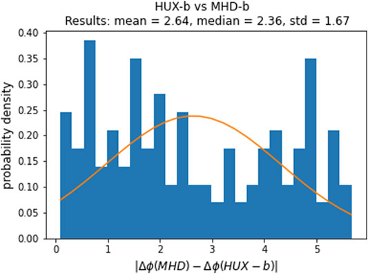
FIGURE 10. Probability density (histogram) of difference between the ballistically mapped longitudes and the MHD-mapped longitudes of the field lines. The blue blocks show the actual frequency while the orange curve provides a Gaussian fit to these data.

3.5 Potential Improvements to the Heliospheric Upwinding eXtrapolation Approach

The HUX approach is simple. In fact, it is probably the simplest physically based improvement to a ballistic approximation that could be made. As noted earlier, several refinements have been made, principally to better address the mixing of temporal and spatial variations at the source. However, here we would like to ask specific questions. First, does differential rotation affect the tuning of the free parameters in the HUX model? Second, does the inclusion of more terms from the momentum equation would improve the approach? And third, is the HUX mapping sensitive to grid resolution?

3.5.1 Effects of Differential Rotation

In paper 1, we estimated the two free parameters of the HUX technique ($\alpha =0.15$ and $r_h=50$) rather subjectively by choosing values that were physically reasonable and produced results that matched with the MHD output at 1 AU for a specific Carrington rotation. We also did not consider the effects of differential rotation on the mapping; a reasonable assumption given the focus on near-equatorial solutions. To address both limitations, we generalized the HUX model to include an angular rotation frequency of the form:

${\text{Ω}}_{rot}\left(\theta \right)=\frac{2\pi }{25.38}-\frac{2.77\pi }{180}cos{\left(\theta \right)}^2(10)$

where θ is colatitude. Thus, at the equator, this produces a rotation rate corresponding to a period of 25.38 days, while at the pole, the period is 31.5 days.

To estimate the error associated with these solutions, we define the residuals between the MHD model (the “data”, or “ground truth” in this case) and the HUX model to be:

$r_i=y_i-f\left(x_i,\alpha ,r_h\right)(11)$

and use the mean square error (MSE) as a measure of the goodness-of-fit of the model:

$MSE=\frac{1}{m}{\displaystyle \sum }_{i=1}^m{r}_i^2(12)$

For CR 2068 (Figure 3), using the values of α and $r_h$ derived in Paper 1, produced a MSE of 3435 over all latitudes and longitudes. By including differential rotation, and allowing the two free parameters to then be optimized, however, we were able to reduce the MSE by a factor of three. We repeated the analysis for a number of other rotations, finding comparable good improvements. However, such optimization is biased in the sense that much of the reduction in error comes from improving the match at mid and high latitudes, and not the equator. When we limited the comparison to the region $\pm {7.25}^{\circ }$ about the heliographic equator, the average optimal α and $r_h$ were found to be 0.16 and 52.6 $R_S$, respectively.

3.5.2 Incorporation of the Pressure Term Into the Heliospheric Upwinding eXtrapolation Model

As shown in paper 1, we could reduce the momentum equation to the inviscid Burgers’ equation under the assumption that the magnetic field, pressure gradient, and gravity can be neglected. But, to what extent is this a reasonable approximation, or, stated another way, what errors are likely introduced? As a secondary question, we can ask whether there is a more speculative formalism that might produce better mappings of the streams from the Sun to 1 AU?

To investigate this, we consider the following generalized expression for $\frac{\partial v_r}{\partial \varphi }$:

$\frac{\partial v_r}{\partial \varphi }=\text{Θ}\xi (13)$

where: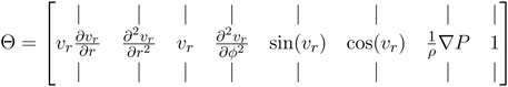(14) Here, $\text{Θ}$ represents the library of potential terms and ξ is a sparse vector containing the optimal coefficients. To build a library of $\text{Θ}$ terms requires us to numerically differentiate the magnetofluid variables. In general, using a central finite difference approach with noisy data would result in terms that are dominated by the amplification of the noise. However, fortunately, since we have smooth-valued MHD solutions, it produces reasonable estimates.

To fully explore the parameter space defined by Eq. 14, we employed the PDE-FIND package, developed by [20]; which searches through a library of terms to fit the optional subset for time-series-like data (or model results).

The details of the analysis are provided in the supplemental information (SI, GitHub), but briefly, we used ridge sparse regression to find the optimal number of terms:

${\xi }^{\text{*}}=argmi{n}_{\xi }\left|\right|\frac{\partial v_r}{\partial \varphi }-\text{Θ}\xi |{|}_2^2+\lambda |\left|\xi \right|{|}_2^2(15)$

The results (SI) showed that the terms $v_r\frac{\partial v_r}{\partial r}$ and $\frac{1}{\rho }\nabla P$ are the most dominant in the library. The resulting equation for CR 2068 was $\frac{\partial v_r}{\partial \varphi }=3.59v_r\frac{\partial v_r}{\partial r}+3.14\frac{1}{\rho }\nabla P$, with a Pearson coefficient of 0.977 and a MSE of 136.0. On the other hand, when excluding $\frac{1}{\rho }\nabla P$ from the library $\text{Θ}$, the resulting underlying equation was $\frac{\partial v_r}{\partial \varphi }=3.398v_r\frac{\partial v_r}{\partial r}$, with a Pearson coefficient of 0.956 and a MSE = 296.1. As an aside, we note that the magnitude of these coefficients makes intuitive sense. The coefficient has units of days/radians, or, the inverse of an angular frequency. During the course of a solar rotation, the implied number of degrees advanced would be: $\left(180/\pi \right)\times 25.38/3.6,or,\sim {400}^{\circ }$. So, at least approximately, the coefficient is consistent with the inverse of the solar rotation rate. Thus, adding $\frac{1}{\rho }\nabla P$ to model solar wind proton velocity, reduced the model’s relative error by 8.65 percent. Repeating this exercise for a total of five rotations, produced relative errors of: 5.8, 8.7, 8.2, 2.9, and 3.1% (CR 2050, 2068, 2100, 2170, and 2231), or, an average relative error of 5.7%. Given the complexity of including the $\nabla P/\rho$ term into the HUX methodology suggests that this modest improvement in accuracy is not worth the cost. Moreover, given the fact that the pressure and density would be very difficult to define at the inner radial boundary, it is not clear that–in practice–the resulting mapping would actually be more accurate. Since the combined ion-electron plasma-β is approximately 2 in the solar wind, this suggests that thermal and magnetic pressures are comparable. Thus, although we have not demonstrated it, we anticipate that the inclusion of magnetic forces would, at best provide a minor improvement that would not be worth the added complexity.

Finally, it is worth noting that PDE-FIND is a physics-agnostic approach, thus, our inclusion of various combinations of first and second-order partial derivatives of was a useful test for validating the approach since it correctly and independently identified the term $v_r\partial v_r/\partial r$ as the dominant term, as well as the secondary contribution from the pressure term, which we had inferred from the full momentum equation. More details outlining this analysis can be found in the SI.

3.5.3 Numerical Convergence of the Heliospheric Upwinding eXtrapolation Mapping

Although the HUX approach is extremely simple, it is still derived from a partial differential equation, and subject to potential convergence issues, such as the Courant–Friedrichs–Lewy (CFL) condition. For the HUX technique, this requires that:

$\frac{\left|v_r\right|\text{Δ}\varphi }{\text{Δ}r{\text{Ω}}_{rot}}\le 1(16)$

In Figure 11 we compare speed traces as a function of longitude for a range of radial resolutions, from a maximum of $n_r=1000$ down to $n_r=n_{min}$, where $n_{min}$ for this case was found to be 32 (below this value no solution could be found). Several points are worth noting. First, resolution does not appear to impact the mappings significantly. There are some systematic differences in moving from the lowest to highest resolutions, but the differences are modest. Second, decreasing the resolution has a tendency of stretching both the peaks and troughs of the profiles, that is increasing the peak speeds and reducing the minimum speeds. On one hand, this could be considered a net improvement for predicting the height of high-speed streams, which tend to be underestimated by the HUX technique; however, it also tends to pull the lowest speeds below those in the “true” MHD solution. The next effect, at least qualitatively, is that any benefits from the two effects would tend to cancel. Overall, then, resolution appears to play a minor role when applying the HUX technique. This may turn out to be important when mapping in situ measurements, particularly inwards, where noise in the highest resolution data may lead to nonphysical artifacts being generated and/or amplified, necessitating some form of smoothing and interpolation onto a coarser mesh.

FIGURE 11

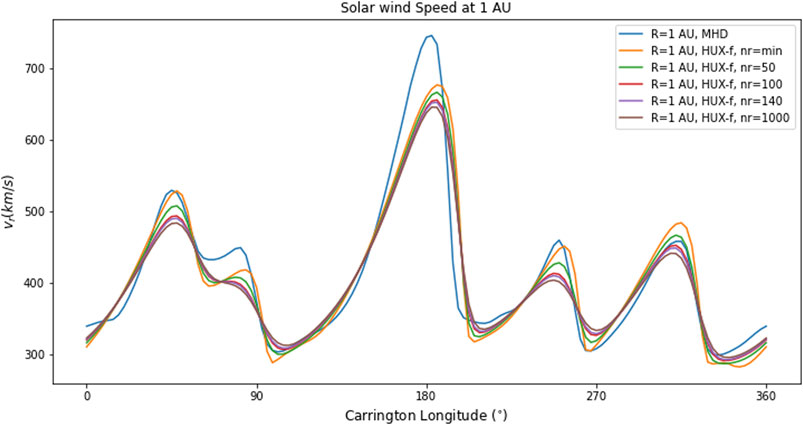
FIGURE 11. Comparison of MHD model speeds with HUX-f solutions of different radial resolution. In this case $n{r}_{min}=32$.

4 Conclusions and Discussion

In this study, we have further developed the Heliospheric Upwinding eXtrapolation (HUX) technique. Specifically, we have: 1) Demonstrated how the approach can be used to map solar wind streams back to the Sun; and 2) Shown that the current formalism is probably as complicated as it needs to be to produce useful results. In addressing these questions, we were able to show how much the HUX technique would improve the accuracy of ballistic mapping studies, which are typically used to identify the source regions of solar wind streams or energetic particles, for example.

This study is not without limitations. In particular, we used MHD model results as the “ground truth”. Although this is reasonable in the sense that we have no other global dataset of solar wind speeds, it assumes that the MHD formalism is accurate enough to evolve solar wind streams through the heliosphere. This, of course breaks down at sufficiently high frequencies. Thus we can only claim that the HUX approach is reasonable on the largest spacial and temporal scales (i.e., macroscopic structure). Additionally, any artifacts introduced by the MHD model, such as numerical diffusion, which are also mimicked by the HUX technique would also contribute to a higher accuracy of the results, but which might not exist in practice. However, given the many studies that have validated the MHD approach for studying solar wind evolution (e.g., [2, 18, 21, 22]), it seems reasonable to conclude that the MHD solutions provide a sufficiently good “ground truth” for such tests.

It is worth noting that our application of PDE-FIND included the viscous term ($\eta {\partial }^2{v}_r/{\partial }^2\varphi$), and this was identified as a contributor when the damping term was small. However, as the damping was increased, it ceased to be important. On average, we estimated that the addition of the viscous term would result in a $\sim 1\text{\%}$ improvement in the linear fit. Thus, we argue that it does not improve the accuracy of the HUX technique sufficiently to merit inclusion. This is consistent with the results of [11] in the sense that they found that it did modify the fit, but did not establish that it made a robust improvement.

In closing, we reiterate that in this study, we have focused on the procedure that could be applied to various in situ datasets, allowing them to be mapped back toward the Sun, or outward from one spacecraft location to another. With the successful launch and commissioning of PSP and Solar Orbiter, as well as the presence of 1 AU spacecraft, including ACE and DSCOVR at Earth, and STEREO-A offset from the Earth Sun line to varying degrees, the technique we have described should be a useful tool for exploring the evolution of streams from one location to another. The approach can also be applied to a broad set of historical datasets including Helios, Ulysses, Pioneer, and Voyagers 1 and 2, just to mention a few. In a future study, we will describe the application of HUX-b and HUX-f to a variety of heliospheric in situ datasets.

Data Availability Statement

The model results used in this study can be found in the HUX repository, located at https://github.com/predsci/HUX.

Author Contributions

PR developed the theoretical formalism for the ideas presented here, with contributions from OI. OI wrote the Python code to test the concepts with minor contributions from PR. PR wrote the paper with input from OI.

Funding

The authors gratefully acknowledge support from NASA (80NSSC18K0100, NNX16AG86G, 80NSSC18K1129, 80NSSC18K0101, 80NSSC20K1285, 80NSSC18K1201, and NNN06AA01C)

Conflict of Interest

Authors PR and OI were employed by Predictive Science Inc.

Acknowledgments

Additionally, the authors would like to express their gratitude to both reviewers for constructive comments that improved the clarity of the manuscript.

References

1. Gosling JT. Corotating and Transient Solar Wind Flows in Three Dimensions. Annu Rev Astron Astrophys (1996) 34:35–73. doi:10.1146/annurev.astro.34.1.35

CrossRef Full Text | Google Scholar

2. Riley P, Linker JA, Mikić Z. An Empirically-Driven Global MHD Model of the Solar Corona and Inner Heliosphere. J Geophys Res (2001) 106:15889–901. doi:10.1029/2000JA000121

CrossRef Full Text | Google Scholar

3. Riley P, Lionello R, Linker JA, Mikic Z, Luhmann J, Wijaya J. Global MHD Modeling of the Solar Corona and Inner Heliosphere for the Whole Heliosphere Interval. Sol Phys (2011b) 274:361–77. doi:10.1007/s11207-010-9698-x

CrossRef Full Text | Google Scholar

4. Riley P, Downs C, Linker JA, Mikic Z, Lionello R, Caplan RM. Predicting the Structure of the Solar Corona and Inner Heliosphere during Parker Solar Probe 's First Perihelion Pass. Astrophysical J Lett (2019) 874:L15. doi:10.3847/2041-8213/ab0ec3

CrossRef Full Text | Google Scholar

5. Riley P, Linker JA, Arge CN. On the Role Played by Magnetic Expansion Factor in the Prediction of Solar Wind Speed. Space Weather (2015) 13:154–69. doi:10.1002/2014sw001144

CrossRef Full Text | Google Scholar

6. Owens MJ, Riley P. Probabilistic Solar Wind Forecasting Using Large Ensembles of Near-Sun Conditions with a Simple One-Dimensional "Upwind" Scheme. Space Weather (2017) 15:1461–74. doi:10.1002/2017sw001679

PubMed Abstract | CrossRef Full Text | Google Scholar

7. Snyder CW, Neugebauer M. The Relation of Mariner-2 Plasma Data to Solar Phenomena. In: RJ Mackin, and M Neugebauer, editors. The Solar Wind. Oxford: Permanon Press (1966). p. 25.

Google Scholar

8. Riley P, Linker JA, Lionello R, Mikic Z. Corotating Interaction Regions during the Recent Solar Minimum: The Power and Limitations of Global MHD Modeling. J Atmos Solar-Terrestrial Phys (2012a) 83:1–10. doi:10.1016/j.jastp.2011.12.013

CrossRef Full Text | Google Scholar

9. Riley P, Lionello R. Mapping Solar Wind Streams from the Sun to 1 AU: A Comparison of Techniques. Sol Phys (2011) 270:575–92. doi:10.1007/s11207-011-9766-x

CrossRef Full Text | Google Scholar

10. Reiss MA, MacNeice PJ, Mays LM, Arge CN, Möstl C, Nikolic L, et al. Forecasting the Ambient Solar Wind with Numerical Models. I. On the Implementation of an Operational Framework. Astrophysical J Suppl Ser (2019) 240:35. doi:10.3847/1538-4365/aaf8b3

CrossRef Full Text | Google Scholar

11. Reiss MA, MacNeice PJ, Muglach K, Arge CN, Möstl C, Riley P, et al. Forecasting the Ambient Solar Wind with Numerical Models. Ii. An Adaptive Prediction System for Specifying Solar Wind Speed Near the Sun. Astrophysical J (2020) 891:165. doi:10.3847/1538-4357/ab78a0

CrossRef Full Text | Google Scholar

12. Bailey RL, Reiss MA, Arge CN, Möstl C, Henney CJ, Owens MJ, et al. Using gradient boosting regression to improve ambient solar wind model predictions. Space Weather (2021). doi:10.1029/2020SW002673

Google Scholar

13. Kumar S, Paul A, Vaidya B. A Comparison Study of Extrapolation Models and Empirical Relations in Forecasting Solar Wind. Front Astron Space Sci (2020) 7:92. doi:10.3389/fspas.2020.572084

CrossRef Full Text | Google Scholar

14. Amerstorfer T, Hinterreiter J, Reiss MA, Möstl C, Davies JA, Bailey RL, et al. Evaluation of Cme Arrival Prediction Using Ensemble Modeling Based on Heliospheric Imaging Observations. Space Weather (2021) 19:e2020SW002553. doi:10.1029/2020sw002553

CrossRef Full Text | Google Scholar

15. Owens M, Lang M, Barnard L, Riley P, Ben-Nun M, Scott CJ, et al. A Computationally Efficient, Time-dependent Model of the Solar Wind for Use as a Surrogate to Three-Dimensional Numerical Magnetohydrodynamic Simulations. Solar Phys (2020) 295:1–17. doi:10.1007/s11207-020-01605-3

CrossRef Full Text | Google Scholar

16. Nolte JT, Roelof EC. Large-scale Structure of the Interplanetary Medium. Sol Phys (1973) 33:241–57. doi:10.1007/bf00152395

CrossRef Full Text | Google Scholar

17. Riley P, Lionello R, Mikić Z, Linker J. Using Global Simulations to Relate the Three‐Part Structure of Coronal Mass Ejections to In Situ Signatures. Astrophysical J (2008) 672:1221–7. doi:10.1086/523893

CrossRef Full Text | Google Scholar

18. Riley P, Stevens M, Linker JA, Lionello R, Mikic Z, Luhmann JG. Modeling the Global Structure of the Heliosphere during the Recent Solar Minimum: Model Improvements and Unipolar Streamers. AIP Conf Proc (2012) 1436:337–43. doi:10.1063/1.4723628

CrossRef Full Text | Google Scholar

19. Riley P. CME Dynamics in a Structured Solar Wind. In: SR Habbal, R Esser, V Hollweg, and PA Isenberg, editors. Solar Wind Nine, Am. Inst. Phys. Conf. Proc. (1999). p. 131

Google Scholar

20. Rudy SH, Brunton SL, Proctor JL, Kutz JN. Data-driven Discovery of Partial Differential Equations. Sci Adv (2017) 3:e1602614. doi:10.1126/sciadv.1602614

PubMed Abstract | CrossRef Full Text | Google Scholar

21. Riley P, Luhmann J, Opitz A, Linker JA, Mikic Z. Interpretation of the Cross-Correlation Function of ACE and STEREO Solar Wind Velocities Using a Global MHD Model. J Geophys Res (2010) 115:11104–+. doi:10.1029/2010JA015717

CrossRef Full Text | Google Scholar

22. Riley P, Lionello R, Caplan RM, Downs C, Linker JA, Badman ST, et al. Using Parker Solar Probe Observations during the First Four Perihelia to Constrain Global Magnetohydrodynamic Models. arXiv preprint arXiv:2102.05101 (2021). doi:10.1051/0004-6361/202039815

CrossRef Full Text | Google Scholar