Infinite Series of Singularities in the Correlated Random Matrices Product

We consider the product of a large number of two 2 × 2 matrices chosen randomly (with some correlation): at any round there are transition probabilities for the matrix type, depending on the choice at previous round. Previously, a functional equation has been derived to calculate such a random product of matrices. Here, we identify the phase structure of the problem with exact expressions for the transition points separating “localized” and “ergodic” regimes. We demonstrate that the latter regime develops through a formation of an infinite series of singularities in the steady-state distribution of vectors that results from the action of the random product of matrices on an initial vector.

1. Introduction

Products of random matrices are one of the most important subjects in the statistical physics of disordered systems [1–8], with a large number of interdisciplinary applications [5]. The continuous distribution of random matrices has been intensively studied in condensed matter physics, see, e.g., references [7, 8], while biological applications typically deal with discrete sets of matrices [9–15]. Another difference is that in the condensed-matter problems the choice of matrices in random products is usually a random process, while for interdisciplinary applications one considers correlations between the choice of matrices at different rounds.

In this paper, we treat the random choice of matrices type as a Markov process. Let us take a reference vector, then consider how the reference vector changes after multiplying it by the random product of n matrices of two types. The vector's norm after n steps is characterized by the Lyapunov exponent for the product of matrices, see reference [16]. In references [17, 18] we gave the semi-analytical solution for the probability distribution for the resulting vector. We derived a system of functional equations, and expressed the maximum Lyapunov index via the steady-state solution of this system of equations.

Previously, a closed functional equation had been obtained in reference [19] for the one-dimensional Ising model in a random magnetic field. Similar functional equations had been derived also in reference [20] to describe the transmission of electrons trough a chain of disordered random scatterers. The main difference between our model and those of reference [20] is that here we consider a correlated choice of matrices, such that the probability of choosing of the next matrix depends on the choice at the last step (“dynamically correlated disorder”), whereas those references studied the case of uncorrelated choice of predefined (static) disorder. Here we identify the phase structure of the correlated random product of matrices, and derive an exact analytical expression for the transition points between different phases of this random product.

Let us now set the stage and specify the model. Consider two 2 × 2 matrices M₀ and M₁. In this paper, we focus on the case of real-valued matrices and vectors. Assume that at the start, we have M₁. We define the transition probabilities q_ij to choose the matrix of type i = 0, 1, when at the previous round we have the matrix of type j = 0, 1. The balance condition for the transition probabilities reads:

$q_{00}+q_{01}=1,q_{10}+q_{11}=1.$

We choose the vector |z₀〉 ≡ (x₀, y₀) at the start and denote the sequence of vectors in the course of evolution as |z_n〉 = (x_n, y_n). We then formulate the following iteration rule to deduce z_n from the values at previous rounds:

$\begin{array}{l}|{\text{z}}_{n+1}\rangle =M_{i_n}|{\text{z}}_n\rangle \equiv M|{\text{z}}_0\rangle ,\\ M={\displaystyle \prod _{k=1}^n}{M}_{i_k}& (1)\end{array}$

for the i_n = 0 or i_n = 1 choices of the matrix type at the n-th round.

It is convenient to introduce the following representation of vector z_n in terms of the polar coordinates:

$\begin{array}{ll}|{\text{z}}_n\rangle =(e^{v_n}cos{\alpha }_n,e^{v_n}sin{\alpha }_n),& (2)\end{array}$

where α is the angle of the vector, and v parameterizes the norm of the vector. We assume that the norm of |z_n〉 grows exponentially with n:

$\begin{array}{ll}\langle {\text{z}}_n|{\text{z}}_n\rangle ~e^{2Rn},& (3)\end{array}$

Then R is identified as the maximum Lyapunov exponent of the matrix product. The main idea of the derivation of R is to consider a correlated random matrix product as a random walk on a two-channel one-dimensional chain.

In addition to the calculation of the Lyapunov exponent, the random product of matrices is characterized by the distribution of angles α_n after nth step (and in the steady state at n → ∞). Below, we will analyze this distribution and identify the phase transition points (depending on the switching probabilities q₀₁ and q₁₀) between the phases where the angles in the steady state remain localized and those where they cover the whole phase space.

The structure of the paper is as follows: in section 2, we briefly overview the main analytical results of reference [17], which will serve as the basis for the following analysis. In section 3.1, we perform a numerical analysis for the case of non-singular matrices. We discuss the phenomenon of emergence of “reflected singularities” in the distribution of angles in section 3.2. In section 3.3, we consider the case of singular matrices. Finally, in section 4, we discuss the obtained results and present the outlook for further studies.

2. The Known Results About the Functional Equation

To describe the random process, we consider an ensemble of the states. We should then look at the probability distribution for the vector z_n or, equivalently, for α_n and v_n. Introducing the master equation for ρ_i(n, α) (where i = 0, 1) describing the distributions of α when the matrix M_i is applied at round n, we derive the following system of functional equations [17]:

$\begin{array}{l}{\rho }_0(n+1,\alpha )=\left[q_{00}{\rho }_0(n,f_0(\alpha ))+q_{01}{\rho }_1(n,f_0(\alpha ))\right]f_0^{\prime }(\alpha ),\\ {\rho }_1(n+1,\alpha )=\left[q_{10}{\rho }_0(n,f_1(\alpha ))+q_{11}{\rho }_1(n,f_1(\alpha ))\right]f_1^{\prime }(\alpha ),& (4)\end{array}$

where we define the functions f_i as

$\begin{array}{l}{f}_i(\alpha )=arccos\frac{{(M_i^{-1})}_{11}cos\alpha +{(M_i^{-1})}_{21}sin\alpha }{\sqrt{\langle \alpha |{(M_i^{-1})}^2|\alpha \rangle }}\\ \text{ for }{(M_i^{-1})}_{21}cos\alpha +{(M_i^{-1})}_{22}sin\alpha \ge 0,& (5)\end{array}$

and

$\begin{array}{l}{f}_i(\alpha )=2\pi -arccos\frac{{(M_i^{-1})}_{11}cos\alpha +{(M_i^{-1})}_{21}sin\alpha }{\sqrt{\langle \alpha |{(M_i^{-1})}^2|\alpha \rangle }},\\ \text{ for }{(M_i^{-1})}_{21}cos\alpha +{(M_i^{-1})}_{22}sin\alpha <0,& (6)\end{array}$

where

$|\alpha \rangle =(cos\alpha ,sin\alpha )$

Assuming a steady-state distribution, we get for such a distribution the set of functional equations

$\begin{array}{l}{\rho }_0(\alpha )=\left[q_{00}{\rho }_1(f_0(\alpha ))+q_{01}{\rho }_2(f_0(\alpha ))\right]f_0^{\prime }(\alpha ),\\ {\rho }_1(\alpha )=\left[q_{10}{\rho }_1(f_1(\alpha ))+q_{11}{\rho }_1(f_1(\alpha ))\right]f_1^{\prime }(\alpha ),& (7)\end{array}$

and calculate the Lyapunov index as [17].

$\begin{array}{ll}R=-{\displaystyle \int }d\alpha \left[{\rho }_0(\alpha )g_0(\alpha )+{\rho }_1(\alpha )g_1(\alpha )\right],& (8)\end{array}$

where the function g_i(α) is given by

$\begin{array}{ll}{g}_i(\alpha )=\frac{1}{2}ln\langle \alpha |{(M_i^{-1})}^2|\alpha \rangle .& (9)\end{array}$

For the case of singular matrices, we use an alternative system of equations:

$\begin{array}{l}{\rho }_0({\bar{f}}_0(\alpha )){\bar{f}}_0^{\prime }(\alpha )=q_{00}{\rho }_0(\alpha )+q_{10}{\rho }_1(\alpha ),\\ {\rho }_1({\bar{f}}_1(\alpha )){\bar{f}}_1^{\prime }(\alpha )=q_{01}{\rho }_0(\alpha )+q_{11}{\rho }_1(\alpha ),& (10)\end{array}$

where the functions ${\bar{f}}_i$ are defined similarly to f_i, with the replacement of matrices $M_i^{-1}$ with M_i:

$\begin{array}{l}{\bar{f}}_i(\alpha )=arccos\frac{{(M_i)}_{11}cos\alpha +{(M_i)}_{21}sin\alpha }{\sqrt{\langle \alpha |{(M_i)}^2|\alpha \rangle }}\\ \text{ for }{(M_i)}_{21}cos\alpha +{(M_i)}_{22}sin\alpha \ge 0,& (11)\end{array}$

and

$\begin{array}{l}{\bar{f}}_i(\alpha )=2\pi -arccos\frac{{(M_i)}_{11}cos\alpha +{(M_i)}_{21}sin\alpha }{\sqrt{\langle \alpha |{(M_i)}^2|\alpha \rangle }},\\ \text{ for }{(M_i)}_{21}cos\alpha +{(M_i)}_{22}sin\alpha <0.& (12)\end{array}$

Similarly, we introduce the function

$\begin{array}{ll}{ḡ}_i(\alpha )=\frac{1}{2}ln\langle \alpha |{(M_i)}^2|\alpha \rangle & (13)\end{array}$

that determines the Lyapunov exponent, as in Equation (8). When deriving Equations (4) and (10), we have assumed a continuous distribution in some interval (that can be the case, e.g., for a continuous distribution of the initial vector z₀), and an asymptotically stable distribution for the steady state.

3. The Phase Structure and Singularities

3.1. The Phase Transitions Between Phases for Non-singular Matrices

For the non-zero transition probabilities, let us first consider the symmetric case q₀₁ = q₁₀ ≡ q. Let us assume that the maximal eigenvalue of the first matrix corresponds to the eigenvector

$\begin{array}{ll}|{\alpha }_0\rangle =(cos{\alpha }_0,sin{\alpha }_0)& (14)\end{array}$

and for the second matrix to the eigenvector

$\begin{array}{ll}|{\alpha }_1\rangle =(cos{\alpha }_1,sin{\alpha }_1)& (15)\end{array}$

We also denote also α₀ = 2πX₀ and α₁ = 2πX₁. For the zero transition rate q = 0, we will have the steady-state distributions

${\rho }_0(\alpha )=\delta (\alpha -{\alpha }_0),{\rho }_1(\alpha )=\delta (\alpha -{\alpha }_1).$

The main question we are going to answer is: How would these angular delta-distributions evolve when the transition rate is non-zero. We start by numerically solving the functional equations for the steady-state angular distributions in the case of non-singular matrices. We take for our numerics the two non-commuting matrices:

$M_0=\left(\begin{array}{cc}3.& 1.\\ 1.& -1.\end{array}\right)$

$M_1=\left(\begin{array}{cc}0.01& 1.01\\ 1.01& 0.01\end{array}\right)$

For q ≪ 1, we observe that ρ₀(α) has a maximum at α₀ and ρ₁(α) has a maximum at α₁, i.e., the delta-distribution for q = 0 are only slightly broadened and remain localized. For our choice of matrices the positions of the maxima are at X₀ = 0.231 and X₁ = 0.785.

With increasing the transition rate q, we encounter different situations. Let us look at the distribution ρ₁(α). For the small transition rates q, we have a peak in Figure 1. This corresponds to the first phase. It disappears while increasing q (Figure 2), and we enter to the second phase (see Figure 3). In the second phase we get a wider distribution for ρ₁. Thus, we observe numerically a transition between the phases where the angular distributions are “localized” and “de-localized” in the phase space.

FIGURE 1

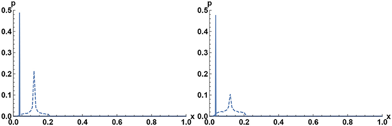
Figure 1. The numerical results for probability distribution of x = α/(2π). The smooth line is ρ₀(x), the dashed line ρ₁(x). (Left) q₀₁ = q₁₀ = 0.005, and (Right) q₀₁ = q₁₀ = 0.010.

FIGURE 2

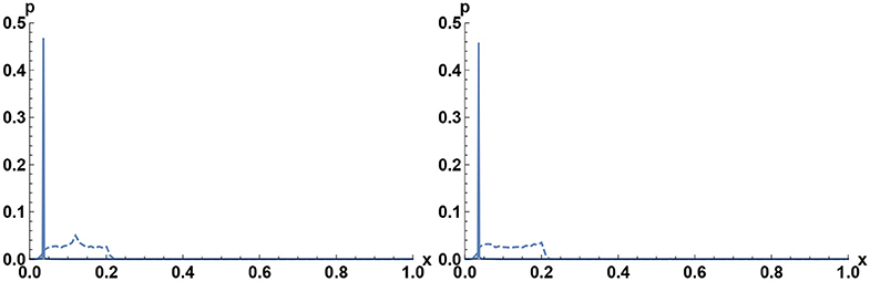
Figure 2. The numerical results for probability distribution of x = α/(2π). The smooth line is ρ₀(x), the dashed line ρ₁(x). (Left) q₀₁ = q₁₀ = 0.015, and (Right) q₀₁ = q₁₀ = 0.020.

FIGURE 3

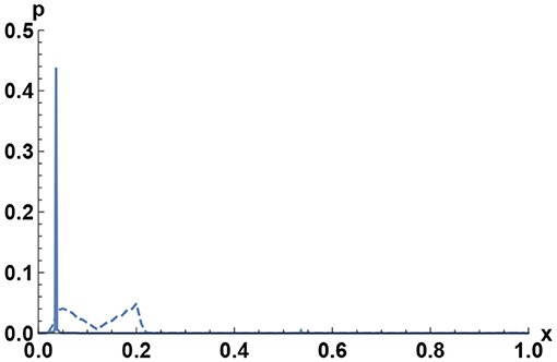
Figure 3. The numerical results for probability distribution of x = α/(2π), q₀₁ = q₁₀ = 0.03. The smooth line is ρ₀(x), the dashed line ρ₁(x).

We can identify the transition point between the first and second phases. Let us assume a singularity of the distribution ρ₁(α) near the point X₁,

$\begin{array}{ll}{\rho }_1(\alpha )~\frac{K_1}{|\alpha -{\alpha }_1{|}^{\gamma }}& (16)\end{array}$

with γ → 1 and K₁ → 0 for q → 0. For q → 0, this distribution becomes a delta-distribution, as it should:

$\begin{array}{ll}{\rho }_1(\alpha )~\frac{ϵ}{|\alpha -{\alpha }_1{|}^{1-ϵ}}{|}_{ϵ\to 0}=\delta (\alpha -{\alpha }_1).& (17)\end{array}$

For the small transition rate for almost diagonal matrices, an exact solution with the scaling singularity has been derived in reference [11], which supports our ansatz. Moreover, this scaling ansatz allows for a correct solution of our functional equation near the singularity point.

Let us denote

$\begin{array}{l}{b}_0={\bar{f}}_0^{\prime }({\alpha }_0),\\ b_1={\bar{f}}_1^{\prime }({\alpha }_1).& (18)\end{array}$

Then we get from the second equation in Equation (7)

$\begin{array}{ll}{(b_1)}^{1-\gamma }=1-q& (19)\end{array}$

and find γ from this equation. The transition point from the behavior by Figure 1 to the one by Figure 2 is at γ = 0,

$\begin{array}{ll}1-q=b_1.& (20)\end{array}$

Equation (20) has a solution for

$\begin{array}{ll}|b_1|<1& (21)\end{array}$

In our case, the transition point for the ρ₁ is at q ≈ 0.02. Figures 1, 2 confirm well this our findings about transition point.

Similarly, we can assume a singular behavior for the distribution ρ₀,

$\begin{array}{ll}{\rho }_0(\alpha )~\frac{K_0}{|\alpha -{\alpha }_0{|}^{\bar{\gamma }}},& (22)\end{array}$

and derive the following expression for the critical index

$\begin{array}{ll}{(b_0)}^{1-\bar{\gamma }}=1-q.& (23)\end{array}$

The transition point is at q = 0.62.

3.2. The Reflected Singularities

In Figure 1 we have single peaks for the distributions (within our accuracy of numerics). In Figures 2, 3, we see several peaks for ρ₁, and many peaks in Figures 4, 5. Further, in Figure 5 we observe five high and eight low peaks in ρ₁. Some of the peaks have identical locations with the peaks in ρ₀, while other peaks have independent locations.

FIGURE 4

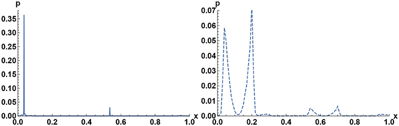
Figure 4. The numerical results for probability distribution of x = α/(2π), q₀₁ = q₁₀ = 0.060. (Left) The smooth line is ρ₀(x), and (Right) the dashed line ρ₁(x).

FIGURE 5

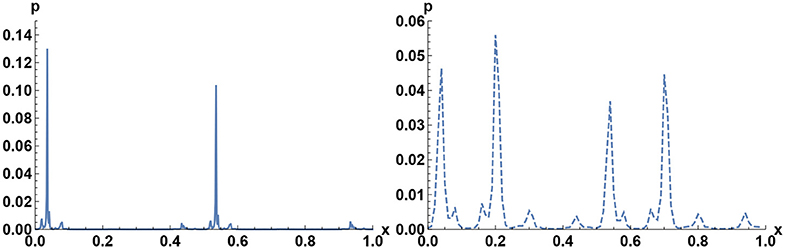
Figure 5. The numerical results for probability distribution of x = α/(2π), q₀₁ = q₁₀ = 0.20. (Left) The smooth line is ρ₀(x), and (Right) the dashed line ρ₁(x).

How can we explain this phenomenon? Here, it is convenient to use the representation of the functional equations for the distributions that we derived for the singular matrices (it is also applicable for the non-singular matrices). Let us look at the distributions near the point α₁ in the equation for ρ₁ and near the point α₀ in the equation for ρ₀. From these equations, we get a new singularity near the point

$\begin{array}{ll}{\alpha }_{01}={\bar{f}}_0({\alpha }_1)& (24)\end{array}$

for ρ₀(α), as well as a new singularity near the point

$\begin{array}{ll}{\alpha }_{10}={\bar{f}}_1({\alpha }_0)& (25)\end{array}$

for ρ₁(α). In fact, iterating this analysis, we find singularities at any of the points

$\begin{array}{ll}{\alpha }_{00..1}={\bar{f}}_0(\dots {\bar{f}}_0({\bar{f}}_0({\alpha }_1)))& (26)\end{array}$

for ρ₀(α), and singularities near the points

$\begin{array}{ll}{\alpha }_{11..0}={\bar{f}}_1(\dots {\bar{f}}_1({\bar{f}}_1({\alpha }_0)))& (27)\end{array}$

for the ρ₁(α).

Consider the case of the power-law singularity addressed above. We assume

$\begin{array}{l}{\rho }_0(\alpha )~\frac{K_{10}}{|\alpha -{\alpha }_{10}{|}^{\bar{\gamma }}},\\ {\rho }_1(\alpha )~\frac{K_{01}}{|\alpha -{\alpha }_{01}{|}^{\gamma }}& (28)\end{array}$

Then we can express K₀₁ and K₁₀ via K₀ and K₁.

In Figure 2, the distribution ρ₁ is just between α₀ and α₁₀. Actually we have peaks for the mixed choice of functions ${\bar{f}}_0,{\bar{f}}_1$ in Equations (26) and (27); only the heights are suppressed via higher powers of q:

$\begin{array}{ll}K~q.& (29)\end{array}$

Let us find the reflected singularities near the point α₁₀. Considering

$\begin{array}{ll}{f}_0(\alpha )\approx f_0({\alpha }_1)+f_0^{\prime }({\alpha }_1)(\alpha -{\alpha }_1),& (30)\end{array}$

we get

$\begin{array}{ll}{K}_{01}=K_1\frac{q}{{\bar{f}}_0{({\alpha }_1)}^{1-\gamma }}.& (31)\end{array}$

In the same way, we get

$\begin{array}{ll}{K}_{10}=K_0\frac{q}{{\bar{f}}_1{({\alpha }_0)}^{1-\bar{\gamma }}}.& (32)\end{array}$

The distribution ρ₁ is extended between α₀ and α₁₀, even after the transition point (see Figure 3).

Then we observe a copy singularities: Further increase of the transition rate brings to the new groups of the peaks (see Figures 4, 5). We can identify the locations of first and second high peaks, then the last peak in Figure 5. We have also done numerical calculations with a different matrix M₀,

$M_0=\left(\begin{array}{cc}1.2& 1.\\ 1.& -1.\end{array}\right)$

getting qualitatively similar results.

3.3. Singular Matrices

We have done numerics for the choice

$M_0=\left(\begin{array}{cc}3.& 1.\\ 1.& -1.\end{array}\right)$

$M_1=\left(\begin{array}{cc}1& 1\\ 1& 1\end{array}\right)$

Let us look at ${\bar{f}}_0^{\prime }(\alpha )$:

The singular case is described by Equation (10). Here, we have a zero value for the derivative of ${\bar{f}}_0^{\prime }$ (see Figure 6), so there is no transition in the behavior of ρ₁(α).

FIGURE 6

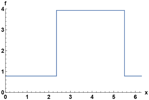
Figure 6. The function $f={\bar{f}}_0(x)$. We take a singular matrix for M₁.

4. Discussion

We have considered the correlated random product of two distinct 2 × 2 matrices, establishing a rich phase structure of the problem. We have identified the transition points between the regimes of “localized” and “extended” behavior of the steady-state distribution of vectors emerging after multiplying an initial vector with an infinite random product of matrices.

Important characteristics of the system are the values of the steady-state vector angle α for the pure case with zero transition rates, α₀ and α₁, corresponding to the maximum eigenvalues of the two matrices involved. For very weak small transition rates, we have two singular power-law distributions, each representing a broadened delta-function around the steady-state values α₀, α₁. We assumed a scaling singularity, as was rigorously derived in reference [10], where an exact solution for the small transition rates was obtained for nearly diagonal matrices. Here, we have assumed such a singular behavior for the general case of matrices M₀ and M₁ that do not commute with each other.

We can define the order parameter of delocalized phase 1/ρ₀(α₀), 1/ρ₁(α₁). They are zero at localized phase, while becoming non-zero in de-localized phase.

Introducing ansatz (16), it is straightforward to identify the critical indices for the angular distributions. While in the related evolution model with the fluctuating fitness landscape (which randomly chooses one of the two landscapes) the distributions of α in the steady state, ρ₀, ρ₁, are located in the interval [α₀, α₁], now the distribution is non-zero outside of these intervals (see Figure 1), with the singularities at α₀ and α₁.

Increasing the transition rates, we enter the phase where ρ₁ is smooth, without any singularity (see Figure 2). We have identified the transition point between the first (“localized”) and second (“extended”) phases. With further increasing the switching probability, we obtain a series of new peaks, one of them at the point near α₀ (Figure 2).

What we have observed, besides the singularities at the points α₀, α₁, is that there is an infinite sequence of singularities, originating from the two original ones. We refer to these emergent singularities as to reflected singularities. It is a general property of functional equations of the type determining the steady-state distributions in the present problem. We have identified the locations of the new singularities, as well as their scaling properties.

We note that the existence of the reflected singularities is a general property of the functional equation, which should be valid in the general case (even when the broadened delta-function is not described by a scaling singularity at small q). We have also performed the numerical calculations for the case when the second matrix is singular. For the chosen case of singular matrix there is no transition to the second phase.

We considered only the case of symmetric transition probabilities. For the asymmetric case the reflected singularities again should exist, only the phase structure will become more complicated. We can apply our functional equation method to solve exactly the general case of diagonal matrices product. Here the distribution could depend on a starting choice of the matrix The reflected singularities should present again, only the phase structure will became more complicated. We hope that the results reported in this paper will further stimulate the advances in this interesting area of statistical physics, having implications on various fields from condensed-matter physics to biological evolution.

Let us briefly describe our simulation code. We first build our functions f,g, and identified steady points f₀(α₀) = α₀, f₁(α₁) = α₁. We consider 500 discrete values of α between α₀, α₁. We considered 20,000 samples of 1,000 iterations. During any iteration we randomly change the type of matrices, depending on the current type.

We are grateful to I. V. Gornyi for interesting discussions and critical remarks on the manuscript, as well as for attracting our attention to reference [20].

Data Availability Statement

The original contributions presented in the study are included in the article/supplementary material, further inquiries can be directed to the corresponding author/s.

Author Contributions

The work has been planned by DS. RP and DS have done the calculations and wrote the article.

Funding

The work was done by the financial support of Russian Science Foundation from the Russian Transport University grant 19-11-00008.

Conflict of Interest

The authors declare that the research was conducted in the absence of any commercial or financial relationships that could be construed as a potential conflict of interest.

The reviewer GJ is currently organizing a Research Topic with one author DS.

Acknowledgments

We thank Igot Gornyi for the discussions.

References

1. Furstenberg H, Kesten H. Products of random matrices. Ann Math Statist. (1960) 31:457. doi: 10.1214/aoms/1177705909

CrossRef Full Text | Google Scholar

2. Bougerol P, Lacroix J. Products of Random Matrices with Applications to Schrodinger Operators. Basel: Birhauser (1985). doi: 10.1007/978-1-4684-9172-2

CrossRef Full Text | Google Scholar

3. Chamayou J, Letac G. Explicit stationary distributions for compositions of random functions and products of random matrices. J Theor Prob. (1991) 4:3. doi: 10.1007/BF01046992

CrossRef Full Text | Google Scholar

4. Crisanti A, Paladin G, Vulpiani A. Products of Random Matrices in Statistical Physics. Berlin: Springer (1993). doi: 10.1007/978-3-642-84942-8

CrossRef Full Text | Google Scholar

5. Comtet A, Luck J, Texier C, Tourigny Y. The lyapunov exponent of products of random 2 × 2 matrices close to the identity. J Stat Phys. (2013) 150:13. doi: 10.1007/s10955-012-0674-8

CrossRef Full Text | Google Scholar

6. Comtet A, Texier C, Tourigny Y. Lyapunov exponents, one-dimensional anderson localisation and products of random matrices. J Phys A. (2013) 46:254003. doi: 10.1088/1751-8113/46/25/254003

CrossRef Full Text | Google Scholar

7. Comtet A, Tourigny Y. Impurity models and products of random matrices. arXiv. (2016) 1601.01822.

Google Scholar

8. Mayer A, Mora T, Rivoire O, Walczak A. Diversity of immune strategies explained by adaptation to pathogen statistics. Proc Natl Acad Sci USA. (2016) 113:8630. doi: 10.1073/pnas.1600663113

PubMed Abstract | CrossRef Full Text | Google Scholar

9. Kussell E, Leibler S. Phenotypic diversity, population growth, and information in fluctuating environments. Science. (2005) 309:2075. doi: 10.1126/science.1114383

PubMed Abstract | CrossRef Full Text | Google Scholar

10. Hufton P, Lin YT, Galla T, McKane A. Intrinsic noise in systems with switching environments. Phys Rev E. (2016) 93:052119. doi: 10.1103/PhysRevE.93.052119

PubMed Abstract | CrossRef Full Text | Google Scholar

11. Skanata A, Kussell E. Evolutionary phase transitions in random environments. Phys Rev Lett. (2016) 117:038104. doi: 10.1103/PhysRevLett.117.038104

PubMed Abstract | CrossRef Full Text | Google Scholar

12. Wienand K, Frey E, Mobilia M. Evolution of a fluctuating population in a randomly switching environment. Phys Rev Lett. (2017) 119:158301. doi: 10.1103/PhysRevLett.119.158301

PubMed Abstract | CrossRef Full Text | Google Scholar

13. Rivoire O, Leibler S. The value of information for populations in varying environments. J Stat Phys. (2011) 142:1124–66. doi: 10.1007/s10955-011-0166-2

CrossRef Full Text | Google Scholar

14. Rivoire O. Informations in models of evolutionary dynamics. J Stat Phys. (2016) 162:1324–52. doi: 10.1007/s10955-015-1381-z

CrossRef Full Text | Google Scholar

15. Allahverdyan AE. Entropy of hidden Markov processes via cycle expansion. J Stat Phys. (2008) 133:535–64. doi: 10.1007/s10955-008-9613-0

CrossRef Full Text | Google Scholar

16. Saakian D. Exact solution of the hidden Markov processes. Phys Rev. (2017) 96:052112. doi: 10.1103/PhysRevE.96.052112

PubMed Abstract | CrossRef Full Text | Google Scholar

17. Saakian D. Semianalytical solution of the random-product problem of matrices and discrete-time random evolution. Phys Rev E. (2018) 98:062115. doi: 10.1103/PhysRevE.98.062115

CrossRef Full Text | Google Scholar

18. Nieuwenhuizen T, Luck J. Semianalytical solution of the random-product problem of matrices and discrete-time random evolution. J Phys A. (1986) 19.

19. Perel V, Polyakov D. Z Eksp Teor Fiz. (1984) 1352–66.

20. Dmitriev A. Transmission of an electron through a finite chain of periodic disordered random scatterers. Z Eksp Teor Fiz. (1984) 95:234–6.