 Mengzhou Li
 Feng-Lei Fan
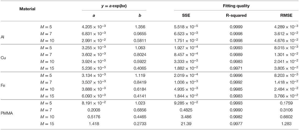

94% of researchers rate our articles as excellent or good
Learn more about the work of our research integrity team to safeguard the quality of each article we publish.
Find out more
ORIGINAL RESEARCH article
Front. Phys., 21 May 2021
Sec. Medical Physics and Imaging
Volume 9 - 2021 | https://doi.org/10.3389/fphy.2021.678171
This article is part of the Research TopicEnergy-Sensitive X-Ray Computed Tomography ImagingView all 9 articles
The energy spectrum of an X-ray tube plays an important role in computed tomography (CT), and is often estimated from physical measurement of dedicated phantoms. Usually, this estimation problem is reduced to solving a system of linear equations, which is generally ill-conditioned. In this paper, we optimize a phantom design to find the most effective combinations of thicknesses for different materials. First, we analyze the ill-posedness of the energy spectrum inversion when the number of unknown variables (N) and measurements (M) are equal, and show the condition number of the system matrix increases exponentially with N if the transmission thicknesses are linearly changed. Then, we present a genetic optimization algorithm to minimize the condition number of the system matrix in a general case (M < N) with respect to the selection of thicknesses and types of phantom materials. Finally, in the simulation with Poisson noise we study the accuracy of the spectrum estimation using the expectation-maximum algorithm. Our results indicate that the proposed method allows high-quality spectrum estimation, and the number of measurements is reduced over two thirds of that required by the widely-used method using a phantom with linearly-changed thicknesses.
Knowledge of the X-ray spectrum plays an important role in all X-ray imaging tasks; e.g., dose calculation [1, 2], dual-energy material decomposition [3], artifacts correction [4], and X-ray detector performance evaluation/calibration [5]. In some cases of a low X-ray flux, the spectrum can be directly measured with an X-ray spectrometer which utilizes energy-resolved detectors. However, besides the cost of the instrument, direct measurement of the energy spectrum of an X-ray source of a high flux can be complicated and difficult. It is well-known that in clinical applications the X-ray source is operated at a relatively high tube current to reduce the scan time. Hence, indirect estimation methods are more practical due to its simplicity. Currently, there are mainly two types of methods for this purpose: estimation via realistic modeling of the source [6], and spectral reconstruction from transmission measurements of calibration phantoms [7].
The modeling method can generate a precise spectrum given all specifications (such as target material, emission angle, and filtration) of the X-ray tube based on a comprehensive physical model of the tube, but in reality this is technically challenging, and we are usually unable to obtain all of the specifications and other details due to the fact that the tube design is often proprietary. Thus, estimation through transmission measurements is more frequently performed. A set of calibration materials with known attenuation properties and thicknesses can be utilized to generate projection data. Then, a group of linear equations of spectral parameters are given based on a discrete polychromatic forward model. The spectrum is finally reconstructed through iterative optimization with regularization [8–10]. This inverse problem is ill-conditioned and even under-determined due to the high dimensionality of the continuous spectrum, making the solution intrinsically unstable. To stabilize the spectral estimation, different techniques were proposed, including a limited-variable representation [11, 12] and mode-combination [13].
In this paper, we focus on reducing the ill-posedness of the problem by improving data quality [14, 15] for estimation robustness, which is complementary with the model-based methods [8, 10, 13, 16]. In practice, aluminum (Al) and polymethyl methacrylate (PMMA) are the most common materials used for spectrum estimation. Step-wedge phantoms or slabs made of those materials are often used to form representative attenuating paths. The measurement process usually involves tens of combinations and takes a long time. However, more combinations do not necessarily reduce the ill-posedness of the problem due to insignificant changes in projection data since small thickness variation of light materials leads to similar attenuation curves. Thus, the investigation for the most effective combinations of different materials and their thicknesses would alleviate the ill-posedness and be beneficial for increased spectrum estimation accuracy with a decreased number of measurements. Here we therefore search for an optimal combination of material types and thicknesses in the set of Al, PMMA, copper (Cu), and iron (Fe). Specifically, we use the Genetic Algorithm (GA) to minimize the condition number of the system matrix and offer guidelines for effective spectral estimation of an X-ray tube. In a simulation study with Poisson noise, we compare the quality metrics of spectrum estimations using our method with the optimized phantom and the conventional method with a linear slab phantom.
Given an X-ray source spectrum distribution S(E) and a detector spectral response D(E), the transmission signal can be formulated as
where Ii represents the intensity of the i-th measurement, and li and μi(E) are the corresponding total path length and linear attenuation coefficient of the involved material, respectively. After flat-field correction and combination of S(E) and D(E) for a normalized spectrum
we can express Equation (1) as
With M measurements, a set of linear equations can be obtained from Equation (3) after evenly discretizing the spectrum into N bins,
where μij denotes μi(Ej), which is the attenuation coefficient within the energy bin. In the matrix form, Equation (4) becomes
where A ∈ ℝM×N with each element being positive, , and .
In conventional practice, the measurements are conducted with a set of attenuation slabs with linearly-changed thicknesses. However, this linear arrangement is not optimal and could lead to the explosion of the condition number of the system matrix A as the number of unknowns becomes large, while a large condition number means an instability of the solution to the system of linear equations.
Let us look at the simplest case of M = N with a single material type. Suppose that the thickness of the slab for i-th measurement is li = l0 + (i − 1)Δl, where l0 is the initial thickness and Δl is a fixed increment. The system matrix in Equation (5) becomes
where μj stands for the linear attenuation coefficient of the material within the j-th energy bin; V and D are respectively an M-by-N Vandermonde matrix and a N-by-N diagonal matrix, and defined as follows:
where . When M = N, A is invertible since det(A) ≠ 0. By definition, the condition number of A is
Without loss of generality, let us look at the conditioning with the infinity norm. Since the ∞-norm of a matrix is equal to the largest 1-norm of rows, suppose that the k-th row of V has the largest 1-norm while the k′-th row of V−1 has the largest 1-norm, which are expressed as
where vi,j and are elements of V and V−1, respectively. Then, we have
and
where di, i ∈ {1, 2, ⋯ , N} are the diagonal elements of D, and , .
By substituting Equations (9) and (10) into Equation (7), we obtain
Since the spectrum is fixed and l0 is a preset constant, the fraction dmin/dmax remains almost constant as N increases (Δl decreases). Hence, the conditioning of A mainly relies on the conditioning of V. However, the Vandermonde matrix is badly conditioned as proven in Gautschi and Inglese [17], and the growth rate of cond∞(V) with N is exponential, and at least O(2N), when with positive node vectors (i.e., xi > 0 for i ∈ {1, …, N}). Thus, the condition number of A gets exponentially increased with N. As a result, we cannot expect to infinitely increase the spectrum estimation resolution by increasing the number of measurements under the configuration of single material with linearly-changed thicknesses.
As shown in Equation (6), the arrangement for linear change in thickness leads to a Vandermonde-like system matrix, which is highly ill-conditioned. Hence, we are motivated to introduce non-linearity, change the matrix form and improve the condition number of the system matrix. Given the complexity of this optimization problem, we use the Genetic Algorithm (GA) [18] to search for an optimal phantom design with respective to material types and thicknesses so that the condition number of the system matrix is minimized. To be practical, we consider a general case of M ≠ N. In this case, the condition number is calculated in the least square sense with the 2-norm:
where A+ is the pseudoinverse of A, and σmax and σmin are the maximum and minimum non-zero singular values of A, respectively. Generally, a genetic algorithm consists of these key steps: chromosome representation, crossover operation, mutation operation, fitness calculation, and selection. Our adapted genetic algorithm is described in the following.
In this application, we code M thicknesses for measurement as a vector l = [l1, l2, …, lM] which represents a chromosome. Each element or gene of a chromosome is bounded within [l0, L] (unit: cm). To ease analysis, the thickness is discretized at a high resolution dl ≪ L. The chromosomes can be initialized with an uniform random number generator within (l0, L), followed by discretization and sorting in an ascending order.
This operation is used to increase the variability of the chromosomes. In this operation, two randomly selected chromosomes from the parent generation are paired to generate two children by mixing the genes from the parents. The generation process includes three steps: first, the positions of the genes to be mixed are randomly selected (each gene position has a 50% chance to be selected); then, the mixing ratio rm ∈ (0, 1) for each selected position is uniformly and randomly generated to mix the parent genes in the position, and two types of new genes are generated following (type-1) and (type-2) where and are two parent genes; finally, two children chromosomes are generated by replacing the genes of parent chromosomes l{a} and l{b} for each and every selected positions with the type-1 and type-2 children genes, respectively. The crossover operation is repeated multiple times according to the product of a pre-defined crossover probability and the population size. The generated children chromosomes are added into the population after all crossover operations are finished.
This operation follows the crossover stage, and increases the gene types of the population via random modification. Each chromosome has a same predefined probability to be mutated. The mutation process consists of following steps: first, one mutation position i is randomly selected for the chromosome; then, the gene on the position li is increased or decreased with equal possibility by a random amount, and specifically, the change is computed as follows:
where rs is a uniformly distributed random scaling factor drawn from (0, 1) for each mutation; and γ is the generation ratio defined by the current number of generations over the maximum number of generations, which helps regulate the converging behavior of the solution.
The fitness is defined by a merit function to determine the quality of each chromosome. Naturally, we use the condition number of the system matrix as the ruler (defined in Equation 6, calculated with l), and calculate the fitness as the negative logarithm of the condition number. The results of the population are then normalized to have a predefined mean and unit variance. The predefined target mean is a hyper-parameter. After the normalization, the negative tail will be truncated to zero.
After the population augmentation via crossover and mutation, the selection operation mimics the natural selection for evolution to control the population size to the predefined level Npop based on the fitness of the chromosomes. The survival chromosomes are randomly selected by repetitively spinning a weighted roulette wheel Npop times. The weight/chance of a chromosome being selected is defined as the fitness of the chromosome over the sum of all fitness of the population. Note that the fitness of the best chromosome is enlarged by several folds (a preset hyper-parameter) before the selection, to adopt the elitism strategy. The thicknesses coded in chromosomes are also sorted in an ascending order after each selection operation to fix the disorder caused during crossover and mutation.
After the chromosome initialization, the genetic operations (crossover, mutation, fitness calculation, and selection) are iterated to reach the maximum number of generations. Then, the best quality solution can be found in the youngest generation. Again, the hyperparameters include the maximum number of generations, the population size, the crossover probability, the mutation probability, the population mean of fitness to be normalized to, and the boosting factor for best chromosomes.
The expectation-maximization (EM) algorithm is widely used for the spectrum estimation to overcome the illness of the problem. It is well-known that the EM method converges to the solution that minimizes the Kullbeck-Liebler distance in the measurement domain. For the problem described in Equation (5), the multiplicative update equation is as follows:
The EM method inherently guarantees a positive spectrum if the initial guess is positive. However, it cannot recover fine details of the spectrum without proper initialization, e.g., missing/distorting characteristic lines, as suggested in Sidky et al. [14]. Hence, we incorporate the positional information of characteristic lines into the initialization for improved performance of the EM estimation. More specifically, all elements of an initial vector are set to 1 except for a few different positive values at the positions of tungsten characteristic peaks.
In this study we limit our scope to measurements with a single material type, as in practice it is common to perform measurements on one step wedge made of the same material. Although a phantom made of multiple materials may improve the condition number of the system matrix, it will be complicated and expensive. To optimize the combination of thicknesses for spectrum estimation, we evaluated each type of the commonly available materials including PMMA, Al, Fe, and Cu. The thickness range was set to [0.02, 10], in the unit of cm, which is practically feasible. The thickness range was discretized at the step of 0.001 cm. The spectral linear attenuation values of the materials were obtained from the database established by National Institute of Standards and Technology (NIST) [19], and are plotted in Figure 1. The values at energy points between the NIST data points were interpolated via log-log cubic-spline fitting, in the same way NIST used for interpolation from measured and calculated data points [20]. Without loss of generality, we considered the spectral range (10, 120 keV) for typical medical CT, with a relatively coarse resolution of 5 keV (i.e., N = 22), and used the mean attenuation value within the energy window of each bin for further calculation. The hyperparameters were empirically set as follows: the maximum number of generations as 500, the population size of 1,000, the crossover probability of 0.65, the mutation probability of 0.1, the target distribution mean of 10, and the best fitness boosting factor of 13. In this scenario, an exemplary cost-generation curve during the search for the optimal solution is shown in Figure 2, with the thickness range of [0, 5] and Al as the phantom material. The smooth convergence of the population average cost and the lowest cost solution from the population demonstrates the appropriateness of the hyperparameter settings.

Figure 1. Spectral linear attenuation coefficients of Al, PMMA, Cu, and Fe, respectively.
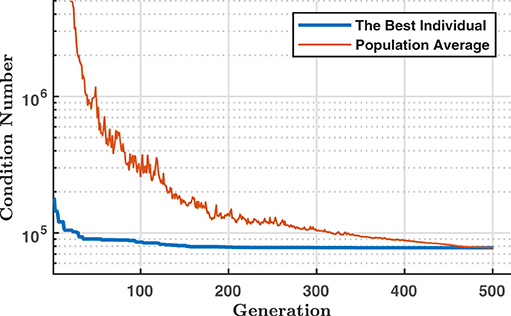
Figure 2. Convergence of the GA optimization in terms of condition number.
We first tested the stability of GA with 200 repetitions of the searching procedure for an optimal set of thicknesses within the range of [0, 5] with nine measurements. One additional open beam (zero thickness) measurement was also included, making the total number of measurements M = 10. The test was conducted with each of the four material types. The results from 200 randomly initialized runs show a great agreement among the solutions. The statistics of the searched thicknesses and the corresponding condition numbers are summarized in Table 1. The standard deviation to mean ratios of the condition numbers are quite small for all four tests, suggesting a high stability/repeatability of GA in this application. As a result, the 200 solutions are extremely close to each other, which implies that we are close to the optimal, since GA often has a good global searching ability.
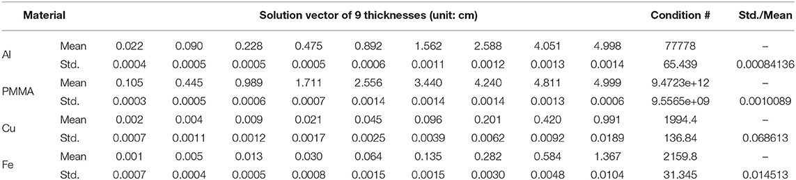
Table 1. Summary of the GA searching results with 200 repetitions when N = 22, l ∈ [0, 5]9.
To investigate the optimal arrangement of thicknesses with a single material type, we first assumed the use of Al which is most popular in step edge phantoms for spectrum estimation. Initially, seven measurements were performed, and thicknesses were searched within [0.02, 10]. The corresponding best linear arrangement was also searched for, as the baseline. For comparison, the first thickness was fixed at 0.02 cm for both linear and non-linear arrangements. In other words, there were 6 thicknesses to be optimized for non-linear arrangement while there was only one variable (i.e., the maximum thickness) to be determined for the linear arrangement. The optimization was repeated 30 times for the non-linear arrangement and 5 times for the linear arrangement, and the smaller number of repetitions for the linear arrangement is due to its high stability. The best solutions among the repetitions are presented in Figure 3B. The standard deviations are close to zero with respect to both the thicknesses and the condition numbers for the optimal non-linear arrangement, suggesting the optimality of the solution. Compared with the best linear arrangement, the condition number is reduced by almost two orders of magnitude with the non-linear scheme.
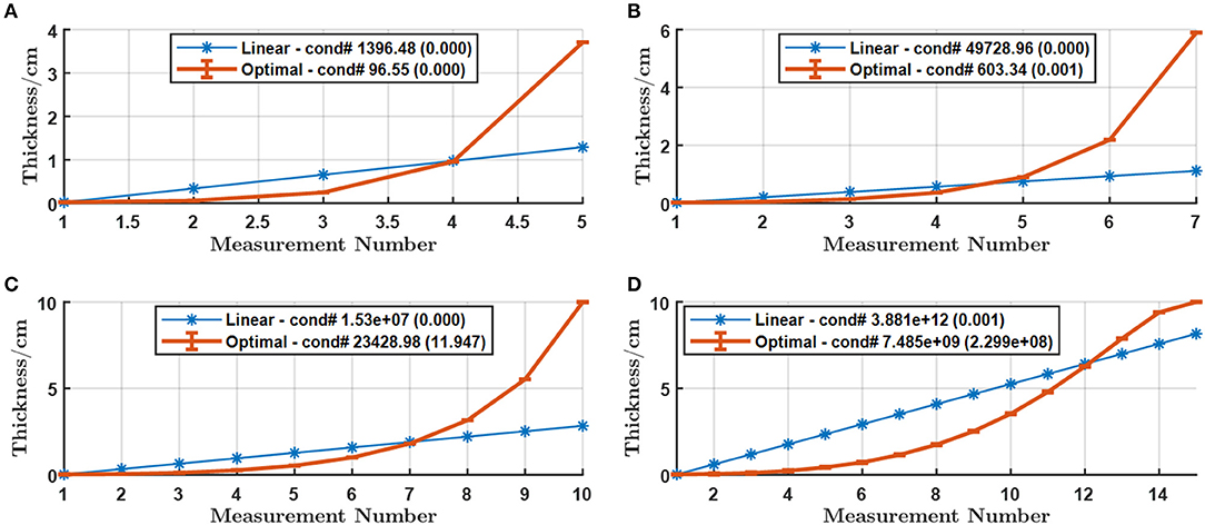
Figure 3. Optimal thicknesses for the non-linear arrangement against the best linear arrangement for (A) M = 5 (B) M = 7 (C) M = 10 and (D) M = 15 measurements with Al within the range [0.02, 10] cm. The error-bars in the curve stand for the standard deviation of the thicknesses while the numbers in the legend are the means and standard deviations of the condition numbers from 30 runs.
One interesting phenomenon in Figure 3B is that both the maximum thicknesses of the best linear and non-linear arrangements do not reach the boundary 10 cm. This suggests that, for a certain number of measurements, blindly increasing the maximum thickness does not necessarily improve the effectiveness of the measurements. This may appear counter-intuitive since a larger thickness makes transmitted X-ray beam harder and hence helps the extraction of spectral information from the measurement, but it is actually reasonable because increasing the thickness also reduces the signal strength, not only saturating the information content but also elevating the instability.
The influence of the number of measurements M was also studied. The total number of measurements was set to 5, 10, and 15, respectively, with the other factors intact. The corresponding results in Figure 3 shows that the condition number rapidly grows as the number of measurements increases. It is also noticed that the shape of the curve in Figure 3D differs from others with the condition number and its standard deviation being very large, but the standard deviations of the thicknesses remain small. This suggests the numerical unstableness due to the bad conditioning of the system matrix. This observation implies that for single material based measurement with a fixed maximum thickness, a few number of measurements should be enough and a larger M would cause a higher instability. Another observation is that the maximum thickness was also changed with the number of measurements in a positively correlated manner.
The impact of material types on optimization results is illustrated in Figures 4–6, corresponding to PMMA, Cu, and Fe, respectively. The figures for Cu and Fe support our conclusions for Al, (1) the condition number improves in orders of magnitude with the non-linear arrangement; (2) the condition number exponentially expands as the number of measurements increases; (3) the maximum thickness increases as the number of measurements increases for both linear and non-linear arrangements. The figure for PMMA does not seem to follow the trends. The condition number expands much faster compared to the cases of the other materials, and the improvement with the non-linear arrangement is still observed but not huge, which can be explained by the maximum thickness being capped by the boundary. Figure 4D even demonstrates unstable optimization results and decreased maximum thickness due to the huge condition number under the capped maximum thickness, making the numerical calculation unstable. When we extended the upper boundary to 100 cm, the searching results become Figure 7, which agrees well with the common trends for the other material types.
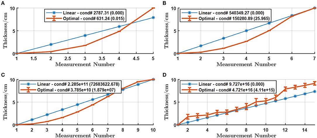
Figure 4. Optimal thickness arrangement against the best linear arrangement for (A) M = 5 (B) M = 7 (C) M = 10 and (D) M = 15 measurements with PMMA within [0.02, 10] cm. The error-bars in the curve stand for the standard deviations of the thickness while the number in parentheses in the legend is the standard deviation of the condition number for 30 repetitions.
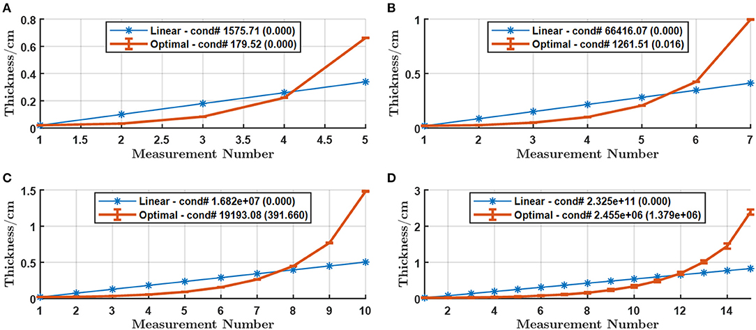
Figure 5. Optimal thickness arrangement against the best linear arrangement for (A) M = 5 (B) M = 7 (C) M = 10 and (D) M = 15 measurements with Cu within [0.02, 10] cm. The error-bars in the curve stand for the standard deviation of the thickness while the number in parentheses in the legend is the standard deviation of the condition number for 30 repetitions.
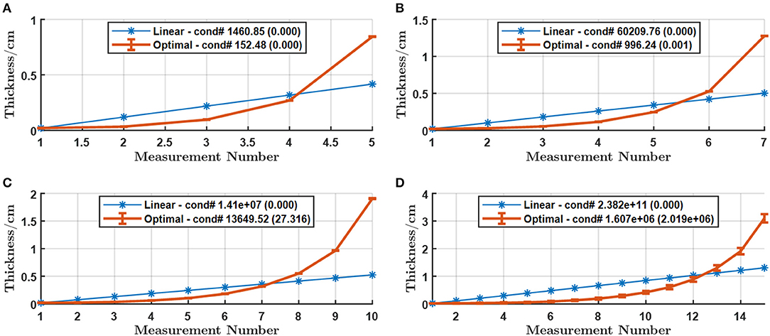
Figure 6. Optimal thickness arrangement against the best linear arrangement for (A) M = 5 (B) M = 7 (C) M = 10 and (D) M = 15 measurements with Fe within [0.02, 10] cm. The error-bars in the curve stand for the standard deviation of the thickness while the number in parentheses in the legend is the standard deviation of the condition number for 30 repetitions.
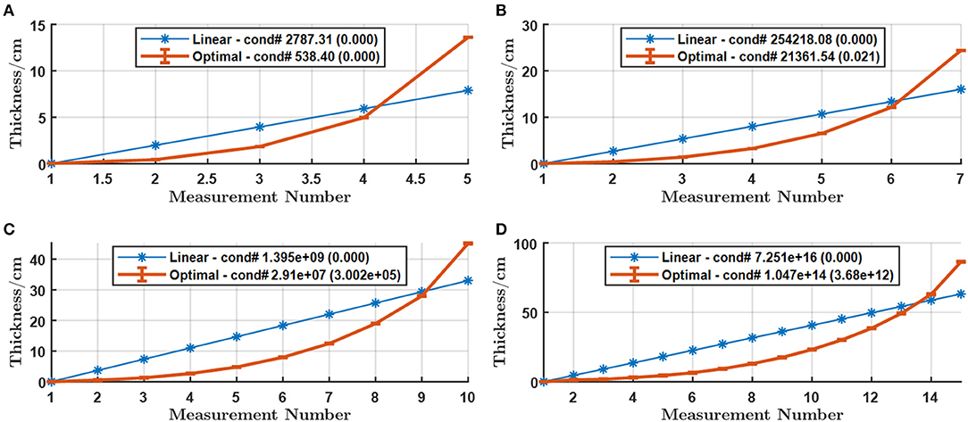
Figure 7. Optimal thickness arrangement against the best linear arrangement for (A) M = 5 (B) M = 7 (C) M = 10 and (D) M = 15 measurements with PMMA within [0.02, 100] cm. The error-bars in the curve stand for the standard deviation of the thickness while the number inside parentheses in the legend is the standard deviation of the condition number for 30 repetitions.
In Figures 3, 5–7, the condition number associated with Al is the smallest when the number of measurements M is no more than 7, but Fe and Cu have much smaller condition numbers when more measurements are allowed. The PMMA has the worst condition number regardless of M, which suggests that PMMA may not be a good material for spectrum estimation. Fe seems to have overall slightly smaller condition numbers than that with Cu. This might be attributed to the 0.2 cm minimum thickness boundary, as we found that Cu has better performance when the range is [0, 5] (see Table 1).
As expected, the maximum thickness depends on not only M but also the material type. Generally, Cu, Fe, Al, and PMMA correspond to increasingly larger maximum thicknesses given the number of measurements, which agrees well with the relative order of their linear attenuation values, as shown in Figure 1. If we compare the results for Al in Table 1 with Figures 3B,D against Figure 3C, as well as Figures 4A–D against each other, we can find that when the maximum thickness is capped, increasing the number of measurements large enough makes the condition number explode. The rapid explosion of the condition number suggests that the increased number of measurements does not introduce more information. Unfortunately, this is the case often seen in practice; i.e., taking many measurements with a relatively small step wedge phantom made of Al, PMMA, or other plastics. Using wedges made of Cu or Fe may help address this issue due to their much smaller maximum thicknesses required to obtain the same number of effective measurements. In addition, if we relax the lower bound of thickness to zero, ten effective measurements can be obtained with Cu and Fe with the condition number being about 2,000 as shown in Table 1.
As projected in the figures, the optimal thickness arrangement is close to an exponential sequence. The results without maximum thickness capping in Figures 3, 5, 7 can be well-fitted into an exponential function, as summarized in Table 2. The Sum of Squares due to Error (SSE), R-square, and Root Mean Squared Error (RMSE) were used to measure the fitting quality. The fitting results demonstrate that the R-squared values are very close to 1, and SSE values are tiny, suggesting the thickness data fit well into an exponential function.
To illustrate the impact of the optimal thickness arrangement on the quality of spectrum estimation, the spectrum estimations from numerically simulated measurements were compared, with three step wedges made of Al, including one conventional phantom and two specifically designed phantoms. The conventional step wedge (or conventional phantom) was simulated with 50 linearly arranged thicknesses ranging from 0.05 to 2.50 cm. One special phantom (the linear phantom) consists of 15 optimized linearly arranged thicknesses while the other wedge phantom (the optimal phantom) consists of 15 optimally arranged thicknesses corresponding to the results in Figure 3D. The tube spectrum was simulated with SpekCalc [6] assuming an operating voltage of 120 kV with a default filter of 0.8 mm Beryllium, 1 mm Al, and 0.11 mm Cu. The spectrum ranges from 12 to 120 keV with a sampling step of 1 keV, resulting in N = 109 energy bins. For simplicity, we assumed a perfect detector and the transmission data were calculated using Equation (5) and only compromised by Poisson noise fPoisson(N0p), where fPoisson denotes the Poisson distribution and N0 stands for the mean number of incident photons. In addition, the tube spectrum is usually measured from a small pencil beam confined with a collimator, which is very similar to the setup for the measurement of the NIST attenuation data [21]. Hence, we did not further consider the scattering (Compton) since it is already included in the LAC data from NIST. The expectation-maximization (EM) algorithm was used for the spectrum reconstruction from the measurements. An all-one vector except for a few different values at positions of tungsten characteristic peaks was used as the initial guess to help the EM method recover the fine details of the spectrum [14]. Two simulated noise levels correspond to the numbers of incident photons and , respectively.
For a quantitative comparison, two common metrics, the normalized root mean squared deviation (NRMSD) and the mean energy difference ΔE were used with definitions as follows:
where ŵ and w are the estimated spectrum and the ground truth, respectively.
The results from the optimal phantom against the linear phantom are shown in Figure 8. Although the two phantoms have the same number of thicknesses, the results of the optimal phantom demonstrate a greater robustness to the noise and the number of iterations as suggested by the stable shape of the estimated spectrum in contrast to the oscillation in the linear phantom results when the noise is stronger or the number of iterations is inadequate. Quantitatively, it can be seen in Figures 8A,C that the results from the optimal phantom are in a better quality especially for stronger noise than that from the linear phantom, also being resilient against inadequate number of iterations. When N0 was increased by 100 times, the Poisson noise became much smaller, and the reconstructions from both phantoms in Figures 8D–F were improved in both metrics relative to those in Figures 8A–C. The results from the optimal phantom were still in a better quality. There is a mismatch near the regions of the characteristic peaks for both phantoms, since the EM method is relatively weak at restoring these high-frequency details.
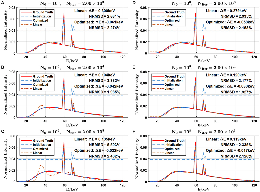
Figure 8. Spectrum estimations from M = 15 optimally arranged thicknesses against M = 15 best linearly arranged thicknesses through Niter iterations under two noise levels characterized by N0, (A) , , (B) , , (C) , , (D) , , (E) , , and (F) , . The initialization is shifted upward by 0.03 for better visibility. The mean energy difference and the NRMSD of the estimated spectra against the ground truth are included.
Similar results from the optimal phantom against those from the conventional phantom are shown in Figure 9. Note that the conventional phantom has M = 50 measurements within the range [0.05, 2.5] while the optimal phantom has much fewer measurements (M = 15) distributed in the range [0.02, 10]. Although the significantly more measurements were made on the conventional phantom, the results are still worse than those from the linear phantom shown in Figure 8, and not even comparable to those from the optimal phantom. This phenomenon illustrates the key point that blindly increasing the number of measurements does not necessarily help the spectrum estimation, while a few well-designed measurements may be effectively enough for the purpose.

Figure 9. Spectrum estimations from M = 15 optimally arranged thicknesses against M = 50 conventional linearly arranged thicknesses through Niter iterations under two noise levels characterized by N0, (A) , , (B) , , (C) , (D) , , (E) , , and (F) , . The initialization is shifted upward by 0.03 for better visibility. The mean energy difference and the NRMSD of the estimated spectra against the ground truth are included.
The combinations of heterogeneous materials has a good potential to achieve better results. We have summarized the best results with individual Al, PMMA, Cu, and Fe materials and five measurements within the range [0, 10] discretized at dl = 0.001 cm in Table 3. As seen in the table, Cu has the smallest condition number around 41.267. When multiple materials are used in the same phantom, the condition number can be further squeezed. By coding the thicknesses of four materials into one chromosome, i.e., l ∈ [0, 10]20, we can search for the potential optimal combinations in a much larger space. Indeed, we have found one combination that has achieved a better result than that with Cu, with a condition number 38.587. However, searching for the optimal solution from a smaller number of measurements is possible but the optimization in the case of a large M is rather difficult since the searching space is exponentially increased according to (L/dl)4M. Due to the huge searching space and limited computing resource, there is a high chance that the iterative process will not converge to the global optimal. Nevertheless, this is a good topic for future research.
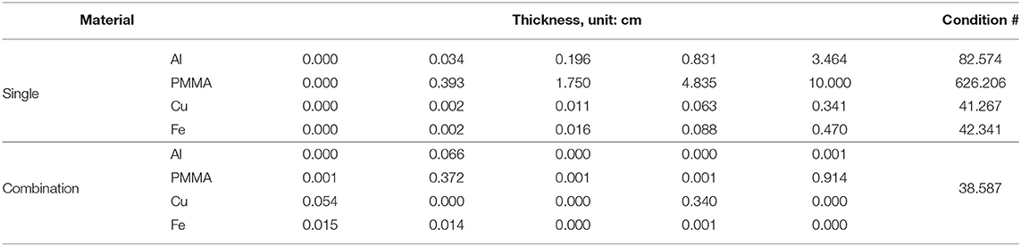
Table 3. Optimal thickness arrangements for M = 5 measurements with each of the material types including Al, PMMA, Cu, and Fe, as well as one exemplary arrangement with the combination of four materials yielding a smaller condition number.
In our model, we have adopted a widely used spectrum model, i.e., decomposing the spectrum into a number of energy bins with equal width using a set of basis functions, such as delta functions [11] or linear B-splines [14]. This method is intuitive but introduces too many unknown variables (equal to the number of bins N), making the inverse problem highly under-determined. Inspired by Zhao et al. [13], we can significantly reduce the degree of freedom by approximating the spectrum as the sum of basis functions in the form of a set of known spectra,
where coefficients ck are the weights over Ns known spectra with different filters. In practice, Ns is often smaller than 10 in contrast to N > 100. Then, the spectrum estimation becomes over-determined. With our optimized thickness arrangement, a significantly reduced number of measurements should result in a more robust and accurate spectrum.
Based on our results, the optimal thickness arrangement should be close to an exponential sequence. However, the commonly available step-wedge phantoms often have the step wedge thicknesses linearly arranged. Here, we suggest two easy-to-implement techniques which can achieve various transmission thicknesses with either slabs or rods. Using a rod with a proper radius r and let an X-ray pencil beam penetrate through the rod with the rod placed perpendicular to the beam propagation direction, then the X-ray path length (i.e., the transmission thickness) can be adjusted by varying the distance d between the pencil beam and the rod center, by lateral translation of the rod, which is expressed as . With a slab of thickness t, by inclining the slab to form an angle θ smaller than 90° with the X-ray beam, the X-ray path length can be computed as t/ cosθ. With these techniques, a series of customized thicknesses can be obtained.
We have studied the optimal thickness arrangement for transmission data measurements with commonly available materials, including Al, PMMA, Cu, and Fe, for high-quality X-ray spectrum estimation, and the condition number of the system matrix has been minimized via genetic evolution. Then, under various conditions the spectra have been estimated via EM iteration. Several interesting observations have been made as follows:
1. Compared with the best linear arrangement of thicknesses, the condition number of the system matrix can be improved by orders of magnitude with the optimal non-linear arrangement;
2. Each material can only support a very limited number of measurements since the condition number exponentially expands as the number of measurements increases;
3. The maximum thickness required by the optimal arrangement increases as the number of measurements increases;
4. The aforementioned maximum thickness also depends on material type, and generally it goes in a descending order for PMMA, Al, Fe, and Cu, whose linear attenuation coefficients become increasingly larger in the order of these material types;
5. Within the maximum thickness, further increasing the number of measurements does not provide more benefit, as indicated by the explosion of the condition number;
6. When the minimum thickness is constrained, e.g., l0 > 0.02 cm, the Al achieves the best result when M ≤ 7, but for larger M, Fe, and Cu are better choices;
7. PMMA has the worst outcome among the four materials regardless of M, which implies that it may not be an appropriate material for this task, although it has been widely used;
8. The optimal thickness arrangement follows an exponential sequence.
The spectrum estimation performance with the EM algorithm has also been studied with the measurements from optimally arranged thicknesses, best linearly arranged thicknesses and conventional linearly arranged thicknesses, with Poisson noise of different levels. The results from the optimal phantom demonstrate a superior performance over the other two in both NRMSD and mean energy difference metrics, demonstrating robustness to noise. These results suggest that with optimized thicknesses and a proper material, the number of measurements can be significantly reduced while still obtaining decent estimation quality. Our future work will consider the combination of different materials per measurement for even better results and the validation with physical experiment data.
The original contributions presented in the study are included in the article/supplementary material, further inquiries can be directed to the corresponding author/s.
The research about X-ray tube spectrum estimation with optimized measurements was proposed by ML. The research funds were provided by GW. The experiments were designed by all authors and carried out by ML. The manuscript was prepared by ML and revised by all authors.
This work was financially supported in part by National Institutes of Health under award numbers R01CA237267 (NCI), R01CA233888 (NCI), R01HL151561 (HHS), and R01EB026646 (NIBIB).
The authors declare that the research was conducted in the absence of any commercial or financial relationships that could be construed as a potential conflict of interest.
The authors would like to thank Shan Gao, Rensselaer Polytechnic Institute, for the help with data fitting work and preparing the summary table.
1. Jarry G, DeMarco J, Beifuss U, Cagnon C, McNitt-Gray M. A Monte Carlo-based method to estimate radiation dose from spiral CT: from phantom testing to patient-specific models. Phys Med Biol. (2003) 48:2645. doi: 10.1088/0031-9155/48/16/306
2. DeMarco J, Cagnon C, Cody D, Stevens D, McCollough CH, O'Daniel J, et al. A Monte Carlo based method to estimate radiation dose from multidetector CT (MDCT): cylindrical and anthropomorphic phantoms. Phys Med Biol. (2005) 50:3989. doi: 10.1088/0031-9155/50/17/005
3. Chang S, Li M, Yu H, Chen X, Deng S, Zhang P, et al. Spectrum estimation-guided iterative reconstruction algorithm for dual energy CT. IEEE Trans Med Imaging. (2019) 39:246–58. doi: 10.1109/TMI.2019.2924920
4. Baer M, Kachelrieß M. Hybrid scatter correction for CT imaging. Phys Med Biol. (2012) 57:6849. doi: 10.1088/0031-9155/57/21/6849
5. Li M, Rundle DS, Wang G. X-ray photon-counting data correction through deep learning. arXiv. (2020) 200703119.
6. Poludniowski G, Landry G, DeBlois F, Evans P, Verhaegen F. SpekCalc: a program to calculate photon spectra from tungsten anode X-ray tubes. Phys Med Biol. (2009) 54:N433. doi: 10.1088/0031-9155/54/19/N01
7. Duan X, Wang J, Yu L, Leng S, McCollough CH. CT scanner X–ray spectrum estimation from transmission measurements. Med Phys. (2011) 38:993–7. doi: 10.1118/1.3547718
8. Leinweber C, Maier J, Kachelrieß M. X–ray spectrum estimation for accurate attenuation simulation. Med Phys. (2017) 44:6183–94. doi: 10.1002/mp.12607
9. Ha W, Sidky EY, Barber RF, Schmidt TG, Pan X. Estimating the spectrum in computed tomography via Kullback–Leibler divergence constrained optimization. Med Phys. (2019) 46:81–92. doi: 10.1002/mp.13257
10. Lee JS, Chen JC. A single scatter model for X-ray CT energy spectrum estimation and polychromatic reconstruction. IEEE Trans Med Imaging. (2015) 34:1403–13. doi: 10.1109/TMI.2015.2395438
11. Ruth C, Joseph PM. Estimation of a photon energy spectrum for a computed tomography scanner. Med Phys. (1997) 24:695–702. doi: 10.1118/1.598159
12. Yang Y, Mou X, Chen X. A robust X-ray tube spectra measuring method by attenuation data. In: Flynn MJ, Hsieh J, editors. Medical Imaging 2006: Physics of Medical Imaging, Vol. 6142. San Diego, CA: International Society for Optics Photonics (2006). p. 61423K. doi: 10.1117/12.654180
13. Zhao W, Niu K, Schafer S, Royalty K. An indirect transmission measurement-based spectrum estimation method for computed tomography. Phys Med Biol. (2014) 60:339. doi: 10.1088/0031-9155/60/1/339
14. Sidky EY, Yu L, Pan X, Zou Y, Vannier M. A robust method of X-ray source spectrum estimation from transmission measurements: demonstrated on computer simulated, scatter-free transmission data. J Appl Phys. (2005) 97:124701. doi: 10.1063/1.1928312
15. Lin Y, Ramirez–Giraldo JC, Gauthier DJ, Stierstorfer K, Samei E. An angle–dependent estimation of CT X–ray spectrum from rotational transmission measurements. Med Phys. (2014) 41:062104. doi: 10.1118/1.4876380
16. Zhao W, Xing L, Zhang Q, Xie Q, Niu T. Segmentation-free X-ray energy spectrum estimation for computed tomography using dual-energy material decomposition. J Med Imaging. (2017) 4:023506. doi: 10.1117/1.JMI.4.2.023506
17. Gautschi W, Inglese G. Lower bounds for the condition number of Vandermonde matrices. Numer Math. (1987) 52:241–50. doi: 10.1007/BF01398878
18. Golberg DE. Genetic algorithms in search, optimization, and machine learning. Addion Wesley. (1989) 1989:36.
19. Hubbell JH, Seltzer SM. Tables of X-Ray Mass Attenuation Coefficients and Mass Energy-Absorption Coefficients (Version 1.4). Gaithersburg, MD: National Institute of Standards Technology (2004). Available online at: http://physics.nist.gov/xaamdi (accessed January 20, 2020).
20. Berger MJ, Hubbell J. XCOM: Photon Cross Sections on a Personal Computer. Washington, DC: National Bureau of Standards; Center for Radiation…(1987). doi: 10.6028/NBS.IR.87-3597
Keywords: spectrum estimation, genetic algorithm, X-ray spectrum, transmission measurement, polychromatic reprojection
Citation: Li M, Fan F-L, Cong W and Wang G (2021) EM Estimation of the X-Ray Spectrum With a Genetically Optimized Step-Wedge Phantom. Front. Phys. 9:678171. doi: 10.3389/fphy.2021.678171
Received: 09 March 2021; Accepted: 15 April 2021;
Published: 21 May 2021.
Edited by:
Liang Li, Tsinghua University, ChinaCopyright © 2021 Li, Fan, Cong and Wang. This is an open-access article distributed under the terms of the Creative Commons Attribution License (CC BY). The use, distribution or reproduction in other forums is permitted, provided the original author(s) and the copyright owner(s) are credited and that the original publication in this journal is cited, in accordance with accepted academic practice. No use, distribution or reproduction is permitted which does not comply with these terms.
*Correspondence: Ge Wang, d2FuZ2c2QHJwaS5lZHU=
Disclaimer: All claims expressed in this article are solely those of the authors and do not necessarily represent those of their affiliated organizations, or those of the publisher, the editors and the reviewers. Any product that may be evaluated in this article or claim that may be made by its manufacturer is not guaranteed or endorsed by the publisher.
Research integrity at Frontiers
Learn more about the work of our research integrity team to safeguard the quality of each article we publish.