Normal Curves in 4-Dimensional Galilean Space G4

In this article, first, we give the definition of normal curves in 4-dimensional Galilean space G⁴. Second, we state the necessary condition for a curve of curvatures τ(s) and σ(s) to be a normal curve in 4-dimensional Galilean space G⁴. Finally, we give some characterizations of normal curves with constant curvatures in G⁴.

1. Introduction

Galilean geometry is one of the Cayley-Klein geometries whose motions are the Galilean transformations of classical kinematics [1]. The Galilean transformation group has an important place in classical and modern physics. It is well known that the idea of world lines originates in physics and was pioneered by Einstein. The world line of a particle is just the curve in space-time which indicates its trajectory [2].

In Euclidean 3-space E³, there are three types of curves, namely, osculating, rectifying, and normal curves [3]. The osculating curve in E³ is defined as a curve whose position vector always lies in its osculating plane, which is spanned by the tangent vector T and the normal vector N [3]. The rectifying curve in E³ is defined as a curve whose position vector always lies in its rectifying plane, which is spanned by the tangent vector T and the binormal vector B. Many researchers have investigated rectifying curves in Euclidean, Lorentz-Minkowski, and Galilean space, as can be seen in [4–6]. Similarly, a normal curve in E³ is defined as a curve whose position vector always lies in its normal plane, which is spanned by the normal vector N and the binormal vector B of the curve. Normal curves in n-dimensional Euclidean space was studied by Ozcan Bekats [7], framed normal curves in Euclidean space was studied by B.D. Yazici, S. O.Karakus, and M. Tosun [8], and normal curves on a smooth immersed surface was investigated by A.A. Shaikh, M.S. Lone, and P.R. Ghosh [9].

There are also many studies related to normal curves in non-Euclidean spaces, for example, normal curves and their characterizations in Lorentzian n-space was studied by Ozgür Boyacıoğlu Kalkan [10] and to the classification of normal and osculating curves in 3-dimensional Sasakian space was studied by M. Kulahck, M. Bahatas, and A. Bilici [11].

In recent years, researchers have begun to introduce curves and surfaces in Galilean and pesedo-Galilean spaces [12–24]. Normal and rectifying curves in Galilean G³ were obtained by Handan Oztekin [25]. Also, many studies about Galilean Geometry were found in Reference [1]. Frenet-Serret frame in the Galilean 4-space was constructed by S.Yilmaz [26].

In the present study, we considered a curve in Galilean 4-space G⁴ whose position vector satisfies the equation α(s) = λ(s)N(s) + μ₁(s)B₁(s) + μ₂(s)B₂(s) for differentiable functions λ(s), μ₁(s), and μ₂(s). N(s), B₁(s), and B₂(s) are normal, first binormal, and second binormal vectors of the curve in Galilean space G⁴. In the first part of the study, the necessary condition for a curve to be a normal curve was obtained; then, we considered a special case when the curvatures are constant and got the position vector of the normal curve in G⁴. At the end of the study, it can be seen that the normal curve in G⁴ lies on a sphere if $\frac{\tau }{\sigma }=$ constant, where τ and σ are the second and the third curvatures of the normal curve α(s).

2. Preliminaries

In this section, we will give some definitions considered in this study. Let $\vec{x}=(x_1,x_2,x_3,x_4)$ and $\vec{y}=(y_1,y_2,y_3,y_4)$ be two vectors in G⁴. The Galilean scalar product in G⁴ is defined by

$<\vec{x},\vec{y}{>}_{G^4}=\{\begin{array}{cc}{x}_1{y}_1,& \mathrm{\text{ if }}{x}_1\ne 0\text{ or }{y}_1\ne 0,\\ x_2{y}_2+x_3{y}_3+x_4{y}_4,& \text{ if }{x}_1=0\text{ and }{y}_1=0.\end{array}$ The norm of the vector $\vec{x}=(x_1,x_2,x_3,x_4)$ is given by $\left|\vec{x}\right|=\sqrt{<\vec{x},\vec{x}{>}_{G^4}}.$

The cross product of any three vectors $\vec{x},$ $\vec{y},$ and $\vec{z}$ in G⁴ is defined by the relation

$\begin{array}{l}\vec{x}\times \vec{y}\times \vec{z}=\{\begin{array}{c}\left|\begin{array}{cccc}0& e_2& e_3& e_4\\ x_1& x_2& x_3& x_4\\ y_1& y_2& y_3& y_4\\ z_1& z_2& z_3& z_4\end{array}\right|,\text{ if }{x}_1\ne 0\text{ or }{y}_1\ne 0\text{ or }{z}_1\ne 0,\\ \\ \left|\begin{array}{cccc}{e}_1& e_2& e_3& e_4\\ x_1& x_2& x_3& x_4\\ y_1& y_2& y_3& y_4\\ z_1& z_2& z_3& z_4\end{array}\right|,\text{ if }{x}_1=y_1=z_1=0,\end{array}\end{array}$

where the unit vectors e₁ = (1, 0, 0, 0), e₂ = (0, 1, 0, 0), e₃ = (0, 0, 1, 0), and e₄ = (0, 0, 0, 1) [1].

A curve α : I ⊂ R → G⁴ of C^∞ in the Galilean space G⁴ is defined by α(t) = (x(t), y(t), z(t), w(t)).

If the curve is parameterized by Galilean arc-length s, it is defined by α(s) = (s, y(s), z(s), w(s)).

The Frenet frame for the parameterized curve α(s) = (s, y(s), z(s), w(s)) in G⁴ is denoted by the following vectors

T(s) = α′(s) = (1, y′(s), z′(s), w′(s)),

$N(s)=\frac{1}{k(s)}{\alpha }^{″}(s)=\frac{1}{k(s)}(0,y^{″}(s),z^{″}(s),w^{″}(s)),$

$B_1(s)=\frac{1}{\tau (s)}(0,{(\frac{y^{″}(s)}{k(s)})}^{\prime },{(\frac{z^{″}(s)}{k(s)})}^{\prime },{(\frac{w^{″}(s)}{k(s)})}^{\prime }),$

B₂(s) = ςT(s) × N(s) × B₁(s),

Here, the coefficient ς is taken ±1 to make the determinant of the matrix [T, N, B₁, B₂] = 1.

where T(s), N(s), B₁(s) and B₂(s) are the tangent, normal, the first binormal, and the second binormal vectors of α(s). k(s) and τ(s) are the first and second curvatures, which are given by the following equations

$k(s)={\left|T^{\prime }(s)\right|}_{G^4}={\left(y^{″}(s)\right)}^2+{\left(z^{″}(s)\right)}^2+{\left(w^{″}(s)\right)}^2,$

$\tau (s)={\left|N^{\prime }(s)\right|}_{G^4}=<N^{\prime }(s),N^{\prime }(s){>}_{G^4}.$

The third curvature of the parameterized curve α(s) is denoted by $\sigma (s)=<B_1^{\prime }(s),B_2(s){>}_{G^4}$. If the curvatures of α(s) are constants, the curve α(s) is called a W-curve. The set {T(s), N(s), B₁(s), B₂(s), k(s), τ(s), σ(s)} is called Frenet apparatus of the curve α(s). The vectors T(s), N(s), B₁(s), and B₂(s) are mutually orthogonal.

$<T(s),T(s){>}_{G^4}=<N(s),N(s){>}_{G^4}=<B_1(s),B_1(s){>}_{G^4}$

$=<B_2(s),B_2(s){>}_{G^4}=1,$

and $<T(s),N(s){>}_{G^4}=<T(s),B_1(s){>}_{G^4}=<T(s),B_2(s){>}_{G^4}=<N(s),B_1(s){>}_{G^4}$

$=<N(s),B_2(s){>}_{G^4}=<B_1(s),B_2(s){>}_{G^4}=0.$

The derivatives of the Frenet equations are defined by [26].

$\begin{array}{l}{T}^{\prime }(s)=k(s)N(s),\\ N^{\prime }(s)=\tau (s)B_1(s),\\ B_1^{\prime }(s)=-\tau (s)N(s)+\sigma (s)B_2(s),\\ B_2^{\prime }(s)=-\sigma (s)B_1(s).& (2.1)\end{array}$

3. Normal Curves in G⁴

In the following section, we will define the normal curves in Galilean 4-dimensional space and prove that there are no congruent curves to the normal curve α(s); finally, we will provide some characterizations of the normal curves in G⁴.

Definition 1. Let α : I ⊂ R → G⁴ be a parameterized curve in G⁴. A curve α(s) is called a normal curve if the orthogonal components of T(s) contains a fixed point for all s ∈ I.

In the following theorem, we indicate the position vector of the normal curve in Galilean 4-space G⁴.

Theorem 1. The position vector of the normal curve in G⁴ with curvatures k(s), τ(s), and σ(s) are defined if τ(s) and σ(s) satisfy the following equations:

$\begin{array}{l}{\left({\mu }_1(s)\right)}^{(r+2)}+{\displaystyle \sum _{k=0}^r{\displaystyle \sum }_{\ell =0}^{r-k}}\left(\begin{array}{c}r+1\\ k\end{array}\right)\left(\begin{array}{c}r-k\\ \ell \end{array}\right)[{\left(\sigma (s)\right)}^{(k)}{\left(\sigma (s)\right)}^{(\ell )}+\\ {\left(\tau (s)\right)}^{(k)}{\left(\tau (s)\right)}^{(\ell )}]{\left({\mu }_1(s)\right)}^{(r-k-\ell )}=0.\end{array}$

Proof: The position vector of a normal curve in G⁴ is defined by

$\begin{array}{ll}\alpha (s)=\lambda (s)N(s)+{\mu }_1(s)B_1(s)+{\mu }_2(s)B_2(s),& (3.1)\end{array}$

where λ(s), μ₁(s), and μ₂(s) are smooth functions of s.

By differentiating (Equation 3.1) with respect to s, we obtain

$\begin{array}{l}{\alpha }^{\prime }(s)={\lambda }^{\prime }(s)N(s)+\lambda (s)N^{\prime }(s)+{\mu }_1^{\prime }(s)B_1(s)+{\mu }_1(s)B_1^{\prime }(s)\\ +{\mu }_2^{\prime }(s)B_2(s)+{\mu }_2(s)B_2^{\prime }(s).& (3.2)\end{array}$

substituting Frenet (Equations 2.1) into Equation 3.2, we have $T(s)=({\lambda }^{\prime }(s)-\tau (s){\mu }_1(s))N(s)+(\lambda (s)\tau (s)+{\mu }_1^{\prime }(s)-{\mu }_2(s)\sigma (s))B_1(s)+({\mu }_1(s)\sigma (s)+{\mu }_2^{\prime }(s))B_2(s).$

Hence, we have the following system of differential equations:

$\begin{array}{ll}\frac{d\lambda }{ds}=\tau (s){\mu }_1(s),& (3.3)\end{array}$

$\begin{array}{ll}\frac{d{\mu }_1}{ds}=-\tau (s)\lambda (s)+\sigma (s){\mu }_2(s),& (3.4)\end{array}$

and

$\begin{array}{ll}\frac{d{\mu }_2}{ds}=-\sigma (s){\mu }_1(s).& (3.5)\end{array}$

Since the curvature functions τ(s) and σ(s) must be differentiable functions, so we consider a set ${F}$ of differentiable functions, defined by

$\begin{array}{ll}{F}=\left\{P_n(s),e^{\omega s},cos\beta s,sin\beta s,n\in \mathbb{N},\omega ,\beta \in ℝ\right\},& (3.6)\end{array}$

where P_n(s) denotes a polynomial function of degree n in s. Here, the curvature functions can be any function of ${F}$, a linear combination or a product of these functions. It is said that ${L}\left[D_s\right]$ annihilates the function ϒ(s) if ${L}\left[D_s\right](\Upsilon (s))=0$. Here, all the member functions of ${F}$ have this property. Consequently, we have two linear differential operators, Φ(D_s) and Ψ(D_s), such that Φ(D_s){τ(s)} = 0 and Ψ(D_s){σ(s)} = 0, where $D_s=\frac{d}{ds}$, some of these annihilator operators are listed in Table 1. By applying the operator Θ(D_s) = Φ(D_s)Ψ(D_s) on Equation (3.4), we have

$\begin{array}{l}\Theta (D_s)D_s{\mu }_1(s)=-\Theta (D_s)\left\{\tau (s)\lambda (s)\right\}+\Theta (D_s)\left\{\sigma (s){\mu }_2(s)\right\}\\ =-\Psi (D_s)\Phi (D_s)\left\{\tau (s)\lambda (s)\right\}\\ +\Phi (D_s)\Psi (D_s)\left\{\sigma (s){\mu }_2(s)\right\}.& (3.7)\end{array}$

The operator Θ(D_s) annihilates the terms that contain λ(s) and μ₂(s), i.e., the right hand side (RHS) of Equation (3.7) contains the derivatives of λ(s) and μ₂(s) from order 1 to an order of less than the order of the derivative of μ₁(s) by 1 at most. Let the maximum derivative in the left hand side (LHS) of Equation (3.7) be r + 1; then, its RHS can be written as a linear combination of the derivatives of τ^(k)(s)λ^{(r − k)}(s) and ${\sigma }^{(k)}(s){\mu }_2^{(r-k)}(s)$ and k ∈ {0, 1, …, r − 1}, consequently, we have

$\begin{array}{l}\Theta (D_s)D_s{\mu }_1(s)={\displaystyle \sum _{k=0}^{r-1}(a_{r,k}{\left(\sigma (s)\right)}^{(k)}{\left({\mu }_2(s)\right)}^{(r-k)}}\\ -b_{r,k}{\left(\tau (s)\right)}^{(k)}{\left(\lambda (s)\right)}^{(r-k)}),& (3.8)\end{array}$

where a_{r, k}, b_{r, k} ∈ ℝ. Next by differentiating Equations (3.3) and (3.5), (r − 1 − k) times and applying Leibniz's rule, one gets

$\begin{array}{l}{\left(\lambda (s)\right)}^{(r-k)}={\left(\tau (s){\mu }_1(s)\right)}^{(r-1-k)}\\ ={\displaystyle \sum _{\ell =0}^{r-1-k}\left(\begin{array}{c}r-1-k\\ \ell \end{array}\right)}{\left(\tau (s)\right)}^{(\ell )}{\left({\mu }_1(s)\right)}^{(r-1-k-\ell )},& (3.9)\end{array}$

and

$\begin{array}{l}{\left({\mu }_2(s)\right)}^{(r-k)}=-{\left(\sigma (s){\mu }_1(s)\right)}^{(r-1-k)}\\ =-{\displaystyle \sum _{\ell =0}^{r-1-k}\left(\begin{array}{c}r-1-k\\ \ell \end{array}\right)}{\left(\sigma (s)\right)}^{(\ell )}{\left({\mu }_1(s)\right)}^{(r-1-k-\ell )}.& (3.10)\end{array}$

Applying Equations (3.9) and (3.10) into (3.8) yields

$\begin{array}{l}\Theta (D_s)D_s{\mu }_1(s)+{\displaystyle \sum _{k=0}^{r-1}{\displaystyle \sum }_{\ell =0}^{r-1-k}}\left(\begin{array}{c}r-1-k\\ \ell \end{array}\right)[a_{r,k}{\left(\sigma (s)\right)}^{(k)}{\left(\sigma (s)\right)}^{(\ell )}+\\ b_{r,k}{\left(\tau (s)\right)}^{(k)}{\left(\tau (s)\right)}^{(\ell )}]{\left({\mu }_1(s)\right)}^{(r-1-k-\ell )}=0.& (3.11)\end{array}$

Equation (3.11) is a linear differential equation of order (r + 1) in μ₁(s) with differential variable coefficients. Its general solution depends on the nature of the coefficients of its derivatives. However, the power series method can be applied to obtain its solution, especially, for any value of s ∈ ℝ is an ordinary point in all the coefficients of the derivatives ${\mu }_1^{(k)}(s)$, k = 0, 1, …, r.

TABLE 1

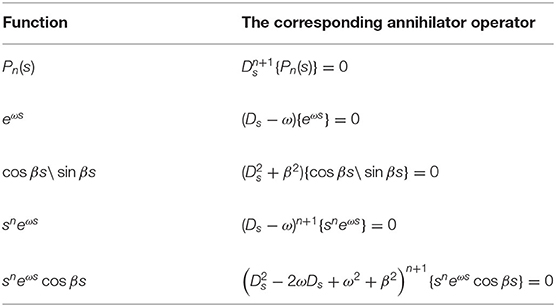
Table 1. Annihilator operators of some functions.

Next, we studied the case when τ(s) ∈ P_n(s) and σ(s) ∈ P_m(s). When r = max(m, n), then the annihilator operator is $D_s^{r+1}$, $D_s^{r+1}\tau (s)=D_s^{r+1}\sigma (s)=0$, and consequently, $\Theta (D_s)=D_s^{r+1}$ was applied into Equation (3.7) by applying Leibniz's rule, yielding

$\begin{array}{l}{\left({\mu }_1(s)\right)}^{(r+2)}={\displaystyle \sum _{k=0}^r\left(\begin{array}{c}r+1\\ k\end{array}\right)}[{\left(\sigma (s)\right)}^{(k)}{\left({\mu }_2(s)\right)}^{(r+1-k)}\\ -{\left(\tau (s)\right)}^{(k)}{\left(\lambda (s)\right)}^{(r+1-k)}].& (3.12)\end{array}$

By using Equations (3.9) and (3.10), Equation (3.12) becomes

$\begin{array}{l}{\left({\mu }_1(s)\right)}^{(r+2)}+{\displaystyle \sum _{k=0}^r{\displaystyle \sum }_{\ell =0}^{r-k}}\left(\begin{array}{c}r+1\\ k\end{array}\right)\left(\begin{array}{c}r-k\\ \ell \end{array}\right)[{\left(\sigma (s)\right)}^{(k)}{\left(\sigma (s)\right)}^{(\ell )}+\\ {\left(\tau (s)\right)}^{(k)}{\left(\tau (s)\right)}^{(\ell )}]{\left({\mu }_1(s)\right)}^{(r-k-\ell )}=0.& (3.13)\end{array}$

Corollary 1. Let α(s) be a normal curve in G⁴. If the curvatures τ (s) and σ(s) ∈ P₁(s), then the position vector of the normal curve in G⁴ is given by

$\begin{array}{l}\alpha (s)=\left(\frac{\pi }{4}\sqrt{2}\left({\left(\text{C}\left(\frac{\sqrt[4]{2}(s+1)}{\sqrt{\pi }}\right)\right)}^2+{\left(\text{S}\left(\frac{\sqrt[4]{2}(s+1)}{\sqrt{\pi }}\right)\right)}^2\right)+c_{\lambda }\right)\\ N(s)+(C_1\sin \left(\frac{\sqrt{2}}{2}{(s+1)}^2\right)+C_2\cos \left(\frac{\sqrt{2}}{2}{(s+1)}^2\right)\\ +C_3\left({{}_{1}F}_2\left[\begin{array}{c}1\\ \begin{array}{cc}\frac{3}{4}& \frac{5}{4}\end{array}\end{array};-\frac{1}{8}{(s+1)}^4\right]\right))\\ B_1(s)+(-\frac{\pi }{4}\sqrt{2}\left({\left(\text{C}\left(\frac{\sqrt[4]{2}(s+1)}{\sqrt{\pi }}\right)\right)}^2+{\left(\text{S}\left(\frac{\sqrt[4]{2}(s+1)}{\sqrt{\pi }}\right)\right)}^2\right)\\ +c_{{\mu }_2})B_2(s)\end{array}$

where C₁, C₂, C₃, c_λ, and c_μ2 are constants; the Fresnel functions, $\text{C}(s)={\int }_0^{s}cos(t^2)dt;andS(s)={\int }_0^{s}sin(t^2)dt;$ the generalized hypergeometric function,

$\begin{array}{}{{}_{p}F}_q\left[\begin{array}{cccc}{\beta }_1& {\beta }_2& \mathrm{...}& {\beta }_p\\ {\gamma }_1& {\gamma }_2& \dots & {\gamma }_q\end{array};s\right]={\displaystyle \sum _{n=0}^{\infty }\frac{{\displaystyle \prod _{j=1}^p{\left({\beta }_p\right)}_n{s}^n}}{{\displaystyle \prod _{j=1}^p{\left({\gamma }_q\right)}_{n}n!}}};\end{array}$

and (β)_n is the shifted factorial, defined by [27]

$\begin{array}{l}{(\beta )}_n=\beta (\beta +1)\dots (\beta +n-1)={\displaystyle \prod _{j=0}^{n-1}}(\beta +j),and{(\beta )}_0=1.\end{array}$

Proof: We consider a special case, when τ(s), σ(s) ∈ P₁(s), i.e., τ(s) = a₁s + b₁, σ(s) = a₂s + b₂, then we have r = 1, ${\tau }^{\prime }(s)=a_1$ and ${\sigma }^{\prime }(s)=a_2$ and the annihilate operator is $D_s^2$ ($D_s^2\tau (s)={\tau }^{″}(s)=D_s^2\sigma (s)=0$); by substituting into Equation (3.13), one gets

$\begin{array}{l}{({\mu }_1(s))}^{(3)}+{\displaystyle \sum _{k=0}^1{\displaystyle \sum }_{\ell =0}^{1-k}}\left(\begin{array}{c}2\\ k\end{array}\right)\left(\begin{array}{c}1-k\\ \ell \end{array}\right)[{(\sigma (s))}^{(k)}{(\sigma (s))}^{(\ell )}\\ +{(\tau (s))}^{(k)}{(\tau (s))}^{(\ell )}]{({\mu }_1(s))}^{(1-k-\ell )}=0.& (3.14)\end{array}$

By extracting the summations, we have

$\begin{array}{l}\frac{d^3{\mu }_1}{d{s}^3}+\left({\left(\sigma (s)\right)}^2+{\left(\tau (s)\right)}^2\right)\frac{d{\mu }_1}{ds}+3(\sigma (s){\sigma }^{\prime }(s)\\ +\tau (s){\tau }^{\prime }(s)){\mu }_1(s)=0.& (3.15)\end{array}$

By applying the power series method to solve Equation (3.15), where ${\mu }_1(s)=\sum _{k=0}^{\infty }{c}_k{s}^k$, differentiating it for up to three times, then substituting into Equation (3.15), and collecting the coefficients, one gets

$\begin{array}{l}{c}_3=\frac{-1}{3!}{\displaystyle \sum _{j=0}^1}(j+1){\varpi }_{1-j}{c}_j,\\ c_4=\frac{1}{2(4!)}{\displaystyle \sum _{j=0}^2}(5j^2-9j-3){\varpi }_{2-j}{c}_j,\\ c_{n+3}=\frac{1}{2{(n+1)}_3}{\displaystyle \sum _{j=0}^2}((5n+3)j^2-(7n+11)j-8(n-1))\\ {\varpi }_{2-j}{c}_{n-1+j},n=2,3,\dots ,\end{array}$

where,

$\begin{array}{l}{\varpi }_0=b_1^2+b_2^2,{\varpi }_1=a_1{b}_1+a_2{b}_2,{\varpi }_2=a_1^2+a_2^2.\end{array}$

Finally, for a special case, when a₁ = a₂ = b₁ = b₂ = 1, the resultant differential equation is

$\begin{array}{ll}{\mu }_1^{″\prime }+2{(s+1)}^2{\mu }_1^{\prime }+6(s+1){\mu }_1=0,& (3.16)\end{array}$

which has the solution ${\mu }_1(s)=C_1\sin \left(\frac{\sqrt{2}}{2}{(s+1)}^2\right)+C_2\cos \left(\frac{\sqrt{2}}{2}{(s+1)}^2\right)+$ $C_3\left({{}_{1}F}_2\left[\begin{array}{c}1\\ \begin{array}{cc}\frac{3}{4}& \frac{5}{4}\end{array}\end{array};-\frac{1}{8}{(s+1)}^4\right]\right).$

It is worth noting that the generalized hypergeometric function is convergent, when p < q + 1, which holds in the proposed problem. Hence, we can obtain the functions λ(s) and μ₂(s), by integrating Equations (3.3) and (3.5) with respect to s, respectively, then we have

$\begin{array}{l}\lambda \left(s\right)=\frac{\pi }{4}\sqrt{2}\left({\left(\text{C}\left(\frac{\sqrt[4]{2}\left(s+1\right)}{\sqrt{\pi }}\right)\right)}^2+{\left(\text{S}\left(\frac{\sqrt[4]{2}\left(s+1\right)}{\sqrt{\pi }}\right)\right)}^2\right)\\ +c_{\lambda },\end{array}$

and

$\begin{array}{l}{\mu }_2\left(s\right)=-\frac{\pi }{4}\sqrt{2}\left({\left(\text{C}\left(\frac{\sqrt[4]{2}\left(s+1\right)}{\sqrt{\pi }}\right)\right)}^2+{\left(\text{S}\left(\frac{\sqrt[4]{2}\left(s+1\right)}{\sqrt{\pi }}\right)\right)}^2\right)\\ +c_{{\mu }_2}.\end{array}$

Corollary 2. The position vector of the normal curve in G⁴ with constant curvatures τ and σ is given by

$\begin{array}{l}\alpha (s)=\left[\frac{\tau }{\sqrt{{\tau }^2+{\sigma }^2}}(c_{1}sin\sqrt{{\tau }^2+{\sigma }^2}s-c_{2}cos\sqrt{{\tau }^2+{\sigma }^2}s)+c_3\right]\\ N(s)+(c_{1}cos\sqrt{{\tau }^2+{\sigma }^2}s+c_{2}sin\sqrt{{\tau }^2+{\sigma }^2}s)B_1(s)+\\ \left[\frac{-\sigma }{\sqrt{{\tau }^2+{\sigma }^2}}(c_{1}sin\sqrt{{\tau }^2+{\sigma }^2}s-c_{2}cos\sqrt{{\tau }^2+{\sigma }^2}s)+c_4\right]B_2(s).\end{array}$

Proof: The position vector of a normal curve in G⁴ is defined by

$\begin{array}{ll}\alpha (s)=\lambda (s)N(s)+{\mu }_1(s)B_1(s)+{\mu }_2(s)B_2(s),& (3.17)\end{array}$

where λ(s), μ₁(s), and μ₂(s) are differentiable functions of s.

By differentiating Equation (3.17) with respect to s, we obtain

$\begin{array}{l}{\alpha }^{\prime }(s)={\lambda }^{\prime }(s)N(s)+\lambda (s)N^{\prime }(s)+{\mu }_1^{\prime }(s)B_1(s)+{\mu }_1(s)B_1^{\prime }(s)\\ +{\mu }_2^{\prime }(s)B_2(s)+{\mu }_2(s)B_2^{\prime }(s).& (3.18)\end{array}$

Substituting Frenet Equations (2.1) into Equation (3.18), we have

$T(s)=({\lambda }^{\prime }(s)-\tau (s){\mu }_1(s))N(s)+(\lambda (s)\tau (s)+{\mu }_1^{\prime }(s)-{\mu }_2(s)\sigma (s))B_1(s)+({\mu }_1(s)\sigma (s)+{\mu }_2^{\prime }(s))B_2(s).$

Hence, we obtain the following differential equations:

$\begin{array}{l}{\lambda }^{\prime }(s)-\tau (s){\mu }_1(s)=0,\\ {\mu }_1^{\prime }(s)+\lambda (s)\tau (s)-{\mu }_2(s)\sigma (s)=0,\\ {\mu }_2^{\prime }(s)+{\mu }_1(s)\sigma (s)=0.& (3.19)\end{array}$

If we take the normal curve α(s) with constant curvatures τ and σ, the Equations (3.19) will take the form

$\begin{array}{l}{\lambda }^{\prime }(s)-\tau {\mu }_1(s)=0,\\ {\mu }_1^{\prime }(s)+\tau \lambda (s)-\sigma {\mu }_2(s)=0,\\ {\mu }_2^{\prime }(s)+\sigma {\mu }_1(s)=0.& (3.20)\end{array}$

By differentiating the second equation of the Equation (3.20) and substituting the first and the third Equation of (3.20), we obtain the following differential equation

$\begin{array}{ll}{\mu }_1^{″}(s)+({\tau }^2+{\sigma }^2){\mu }_1(s)=0.& (3.21)\end{array}$

By solving the ordinary differential Equation (3.21), we obtain

$\begin{array}{ll}{\mu }_1(s)=c_{1}cos\sqrt{{\tau }^2+{\sigma }^2}s+c_{2}sin\sqrt{{\tau }^2+{\sigma }^2}s,& (3.22)\end{array}$

$\begin{array}{l}\lambda (s)=\tau {\displaystyle \int {\mu }_1}(s)ds=\frac{\tau }{\sqrt{{\tau }^2+{\sigma }^2}}(c_1\sin \sqrt{{\tau }^2+{\sigma }^2}s\\ -c_2\cos \sqrt{{\tau }^2+{\sigma }^2}s)+c_3,& (3.23)\end{array}$

$\begin{array}{l}{\mu }_2(s)=-\sigma {\displaystyle \int {\mu }_1}(s)ds=\frac{-\sigma }{\sqrt{{\tau }^2+{\sigma }^2}}(c_1\sin \sqrt{{\tau }^2+{\sigma }^2}s\\ -c_2\cos \sqrt{{\tau }^2+{\sigma }^2}s)+c_4,& (3.24)\end{array}$

where c₁, c₂, c₃ and c₄ are constants.

In the following corollary, we give some characterizations for the curve to be a normal curve.

Corollary 3. Let α(s) be a normal curve in Galilean 4- space G⁴ with non-zero constant curvatures τ and σ. The following statements are satisfied.

1. <$\alpha (s),N(s)>=\frac{\tau }{\sqrt{{\tau }^2+{\sigma }^2}}(c_{1}sin\sqrt{{\tau }^2+{\sigma }^2}s-c_{2}cos\sqrt{{\tau }^2+{\sigma }^2}s)$ + c₃,

2. <$\alpha (s),B_1(s)>=c_{1}cos\sqrt{{\tau }^2+{\sigma }^2}s+c_{2}sin\sqrt{{\tau }^2+{\sigma }^2}s,$

3. <$\alpha (s),B_2(s)>=\frac{-\sigma }{\sqrt{{\tau }^2+{\sigma }^2}}(c_{1}sin\sqrt{{\tau }^2+{\sigma }^2}s-c_{2}cos\sqrt{{\tau }^2+{\sigma }^2}s)$ + c₄,

where c₁, c₂, c₃, and c₄ are constants.

Proof: Suppose that α(s) is a normal curve in Galilean 4-space G⁴ with non-zero constant curvatures τ and σ, then α(s) can be written in the form

α $(s)=(\frac{\tau }{\sqrt{{\tau }^2+{\sigma }^2}}(c_{1}sin\sqrt{{\tau }^2+{\sigma }^2}s-c_{2}cos\sqrt{{\tau }^2+{\sigma }^2}s)+c_3)$

$N(s)+(c_{1}cos\sqrt{{\tau }^2+{\sigma }^2}s+c_{2}sin\sqrt{{\tau }^2+{\sigma }^2}s)B_1(s)+$

$(\frac{-\sigma }{\sqrt{{\tau }^2+{\sigma }^2}}(c_{1}sin\sqrt{{\tau }^2+{\sigma }^2}s-c_{2}cos\sqrt{{\tau }^2+{\sigma }^2}s)+c_4)B_2(s).$

Taking the inner product of the two sides with N(s), B₁(s), and B₂(s), the statements are held.

In the following theorem, we prove that, if α(s) is a normal curve, there are no curves which are congruent to α(s).

Theorem 2. Let α(s) be a normal curve in Galilean space G⁴ with non-zero constant curvatures τ and σ. Then, there are no curves which are congruent to α(s).

Proof: First, let us define m(s) as follows

$\begin{array}{ll}m(s)=\alpha (s)-\lambda (s)N(s)-{\mu }_1(s)B_1(s)-{\mu }_2(s)B_2(s).& (3.25)\end{array}$

Taking the derivative of Equation (3.25) for both sides, we obtain

$m^{\prime }(s)=T(s)-\left[{\lambda }^{\prime }(s)N(s)+\lambda (s)N^{\prime }(s)+{\mu }_1^{\prime }(s)B_1(s)+{\mu }_1(s)B_1^{\prime }(s)+{\mu }_2^{\prime }(s)B_2(s)+{\mu }_2(s)B_2^{\prime }(s)\right].$

By substituting from Equations (2.1), (3.22)–(3.24).

$m^{\prime }(s)=T(s)-[(c_1\cos \sqrt{{\tau }^2+{\sigma }^2}s+c_2\sin \sqrt{{\tau }^2+{\sigma }^2}s)N(s)+$ $(\frac{\tau }{\sqrt{{\tau }^2+{\sigma }^2}}(c_1\sin \sqrt{{\tau }^2+{\sigma }^2}s-c_2\cos \sqrt{{\tau }^2+{\sigma }^2}s)+c_3)(\tau B_1(s))+$ $(-c_1\sqrt{{\tau }^2+{\sigma }^2}\sin \sqrt{{\tau }^2+{\sigma }^2}s+$ $c_2\sqrt{{\tau }^2+{\sigma }^2}\cos \sqrt{{\tau }^2+{\sigma }^2}s)B_1(s)$ $+(c_1\cos \sqrt{{\tau }^2+{\sigma }^2}s+c_2\sin \sqrt{{\tau }^2+{\sigma }^2}s)(-\tau N(s)+\sigma B_2(s))$ $+(-c_1\sigma \cos \sqrt{{\tau }^2+{\sigma }^2}s-c_2\sigma \sin \sqrt{{\tau }^2+{\sigma }^2}s)B_2(s)$ $+((\frac{-\sigma }{\sqrt{{\tau }^2+{\sigma }^2}}(c_1\sin \sqrt{{\tau }^2+{\sigma }^2}s+c_2\cos \sqrt{{\tau }^2+{\sigma }^2}s)+c_4)(-\sigma B_1(s))]$

$m^{\prime }(s)=T(s)+(-\tau c_3+\sigma c_4)B_1(s)$

m′(s) does not equal to zero, which means that m(s) is not a constant vector. So, α(s) is not congruent to a normal curve.

In the following theorem, we give the necessary condition for the normal curve in Galilean 4-space to lie on a sphere.

Theorem 3. Let α(s) be a normal curve in Galilean 4-space G⁴ with non-zero constant curvatures τ and σ. Then, α(s) lies on a sphere if $\frac{\tau }{\sigma }=\frac{c_4}{c_3}$, where c₃ and c₄ are the constants in equations (3.23) and (3.24).

Proof: The inner product of the position vector of α(s) is defined by

g( α(s), α(s)) = < α(s), $\alpha (s){>}_{G^4}$

$={(\frac{\tau }{\sqrt{{\tau }^2+{\sigma }^2}}(c_{1}sin\sqrt{{\tau }^2+{\sigma }^2}s-c_{2}cos\sqrt{{\tau }^2+{\sigma }^2}s)+c_3)}^2+$

${(c_{1}cos\sqrt{{\tau }^2+{\sigma }^2}s+c_{2}sin\sqrt{{\tau }^2+{\sigma }^2}s)}^2+$

${(\frac{-\sigma }{\sqrt{{\tau }^2+{\sigma }^2}}(c_{1}sin\sqrt{{\tau }^2+{\sigma }^2}s-c_{2}cos\sqrt{{\tau }^2+{\sigma }^2}s)+c_4)}^2.$

By simple computations, we have

< α(s), $\alpha (s){>}_{G^4}=(c_1^2+c_2^2+c_3^2+c_4^2)+(\frac{2c_1{c}_3\tau -2c_1{c}_4\sigma }{\sqrt{{\tau }^2+{\sigma }^2}})sin\sqrt{{\tau }^2+{\sigma }^2}s+$

$(\frac{-2c_2{c}_3\tau +2c_2{c}_4\sigma }{\sqrt{{\tau }^2+{\sigma }^2}})cos\sqrt{{\tau }^2+{\sigma }^2}s.$

If $\frac{\tau }{\sigma }=\frac{c_4}{c_3}$, then < α(s), $\alpha (s){>}_{G^4}=(c_1^2+c_2^2+c_3^2+c_4^2)$, which means that α(s) lies on a sphere.

4. Conclusion

In this study, we established the definition of the normal curve in Galilean 4- space G⁴. Also, we derived the necessary condition for a curve to be a normal curve in G⁴. We have proved that, if α(s) is a normal curve in G⁴ with constant curvatures, there is no curve which is congruent to α(s). In the end, the necessary condition for a normal curve to lie on a sphere has been obtained.

Data Availability Statement

The original contributions presented in the study are included in the article/supplementary materials, further inquiries can be directed to the corresponding author/s.

Author Contributions

All authors listed have made a substantial, direct and intellectual contribution to the work, and approved it for publication.

Conflict of Interest

The authors declare that the research was conducted in the absence of any commercial or financial relationships that could be construed as a potential conflict of interest.

Acknowledgments

The authors wish to express their sincere thanks to referee for making several useful comments that improved the first version of the paper.

References

1. Yaglom IM. A Simple Non-Euclidean Geometry and Its Physical Basis. New York, NY: Springer-Verlag (1979).

Google Scholar

2. Epstein M. Differential Geometry Basic Notions and Physical Examples. Switzerland: Springer International Publishing (2014).

Google Scholar

3. Docarmo MP. Differential Geometry of Curves and Surfaces. Rio de Jaeiro: Instituto de Matematica Pure e Aplicada (IMPA) (1976).

Google Scholar

4. Cambie S, Goemans W, Bussche IV. Rectifying curves in the n-dimensional Euclidean space. Turk J Math. (2016) 40:210–23. doi: 10.3906/mat-1502-77

CrossRef Full Text | Google Scholar

5. Ilarslan K, Nesovic E, Torgasev MP. Some Characterizations of rectifying curves in the Minkowski 3- space. Novi Sad J Math. (2003) 33:23–32.

Google Scholar

6. Lone MS. Some characterizations of rectifying curves in four dimensional Galilean space G4. Glob J Pure Appl Math. (2017) 13:579–87.

Google Scholar

7. Bektas O. Normal curves in n-dimensional Euclidean space. Adv Diff Equat. (2018) 2018:456. doi: 10.1186/s13662-018-1922-2

CrossRef Full Text | Google Scholar

8. Yazici BD, Karakus SO, Tosun M. Framed normal curves in Euclidean space. Tbilisi Math. J. (2021) 27–37. doi: 10.2478/9788395793882-003

CrossRef Full Text

9. Shaikh AA, Lone MS, Ghosh PR. Normal curves on a smooth Immersed surface. Ind J Pure Appl Math. (2020) 51:1343–55. doi: 10.1007/s13226-020-0469-6

CrossRef Full Text | Google Scholar

10. Kalkan OB. On normal curves and their characterizations in Lorentzian n-space. AIMS Math. (2020) 5:3510–24. doi: 10.3934/math.2020228

CrossRef Full Text | Google Scholar

11. Kulahci MA, Bektas M, Bilici A. On classification of normal and osculating curve in 3-dimensional Sacakian space. Math sci Appl E-Notes (2019) 7:120–27. doi: 10.36753/mathenot.521075

CrossRef Full Text | Google Scholar

12. Abdel-Aziz HS, Saad MK. Darboux frames of bertrand curves in the Galilean and Pseudo-Galilean spaces. JP J Geometry Topol. (2014)16:17–43.

13. Dede M, Ekici C. On parallel ruled surfaces in Galilean space. J Math. (2016) 40:47–59. doi: 10.5937/KgJMath1601047D

CrossRef Full Text | Google Scholar

14. Aydin ME, Ogrenmis AO. Spherical product surfaces in the Galilean space. J Math. (2016) 4:290–8.

Google Scholar

15. Dede M. Tubuler surfaces in Galilean space. Math Commun. (2013) 18:209–17.

Google Scholar

16. Dede M, Ekici C, Coken A. On the parallel surfaces in Galilean space. J Math Stat. (2013) 42:605–15. doi: 10.15672/HJMS.2014437520

CrossRef Full Text | Google Scholar

17. Elzawy M, Mosa S. Smarandache curves in the Galilean 4-Space G₄. J Egypat Math Soc. (2017) 25:53–6. doi: 10.1016/j.joems.2016.04.008

CrossRef Full Text | Google Scholar

18. Elzawy M, Mosa S. Quaternionic bertrand curves in the Galilean space. Filomat. (2020) 34:59–66. doi: 10.2298/FIL2001059E

CrossRef Full Text | Google Scholar

19. Bektas M, Ergut M, Ogrenmus AO. Special curves of 4D Galilean space. Int J Math Eng Sci. (2013) 2. doi: 10.1155/2014/318458

CrossRef Full Text

20. Oztekin H, Tatlipinar S. Determination of the position vectors of curves from Intrinsic Equations in G₃. J Sci Tech. (2014) 11:1011–1018. doi: 10.14456/372

CrossRef Full Text | Google Scholar

21. Elzawy M. Hasimoto surfaces in Galilean space G₃. J Egypat Math Soc. (2021) 29:1–9. doi: 10.1186/s42787-021-00113-y

CrossRef Full Text | Google Scholar

22. Yoon DW, Lee JW, Lee CW. Osculating curves in the Galilean 4- space. Int J Pure Appl Math. (2015) 100:497–506. doi: 10.12732/IJPAM.V100I4.9

CrossRef Full Text | Google Scholar

23. Elzawy M, Mosa S. Razzaboni surfaces in the Galilean Space G³, far east. J Math Sci. (2018) 108:13–26. doi: 10.17654/MS108010013

CrossRef Full Text

24. Mosa S, Elzawy M. Helicoidal surfaces in Galilean Space with density. Front. Phys. 8:81. doi: 10.3389/fphy.2020.00081

CrossRef Full Text | Google Scholar

25. Oztekin H. Normal and rectifying curves in Galilean G₃. Proc IAM. (2016) 5:98–109.

Google Scholar

26. Yılmaz S. Construction of the Frenet-Serret frame of a curve in 4D Galilean space and some applications. Int J Phys Sci. (2010) 5:1284–9.

Google Scholar

27. Andrews GE, Askey R, Roy R. Special Functions. Cambridge University Press (1999).

Google Scholar