
ORIGINAL RESEARCH article

Front. Phys., 19 July 2021
Sec. Interdisciplinary Physics
This article is part of the Research Topic Classical Statistical Mechanics Using Confined Brownian Particles View all 9 articles

Coarse Graining Nonisothermal Microswimmer Suspensions

  • 1Institute for Theoretical Physics, University of Leipzig, Leipzig, Germany
  • 2Department of Physics, Indian Institute of Science Education and Research, Mohali, India
  • 3Department of Physics and Materials Science, University of Luxembourg, Luxembourg, Luxembourg

We investigate coarse-grained models of suspended self-thermophoretic microswimmers. Upon heating, the Janus spheres, with hemispheres made of different materials, induce a heterogeneous local solvent temperature that causes the self-phoretic particle propulsion. Starting from molecular dynamics simulations that schematically resolve the molecular composition of the solvent and the microswimmer, we verify the coarse-grained description of the fluid in terms of a local molecular temperature field, and its role for the particle’s thermophoretic self-propulsion and hot Brownian motion. The latter is governed by effective nonequilibrium temperatures, which are measured from simulations by confining the particle position and orientation. They are theoretically shown to remain relevant for any further spatial coarse-graining towards a hydrodynamic description of the entire suspension as a homogeneous complex fluid.

1 Introduction

Mesoscale phenomena are at the core of current research in hard and soft matter systems [1, 2]. The reason for this is at least twofold. Firstly, some of the most interesting states of matter are not properties of single atoms or elementary particles, but emerge from many-body interactions, at the mesoscale; e.g., the mechanical strength of many materials is determined by low-dimensional mesostructures. Secondly, these interesting mesoscale properties are often insensitive to molecular details and amenable to widely applicable coarse-grained models that provide both physical insight and efficient control [3]. Extensive atomistic computer simulations can therefore usually be bypassed either by much more efficient coarse-grained numerical techniques [46] or even by analytical methods [7, 8]. Both exploit the universality of the mesoscale physics to compute experimental observables without having to resolve the atomistic details. The price one pays for this efficiency is that fluctuations, which are increasingly important in biophysical and nanotechnological applications [913], may get renormalized or even inadvertently lost upon coarse graining. It is then not always obvious how they have to be properly re-introduced when need arises [14]. Systems with non-equilibrium mesoscale fluctuations, such as suspensions of self-propelled particles and other active fluids [15, 16], are of particular interest in this respect.

One might imagine an approach based on non-equilibrium thermodynamics, which, like hydrodynamics itself, is often valid down to the nanoscale, if judiciously applied [17]. But this theory’s starting point is a macroscopic deterministic one, without fluctuations, so that it is natively blind to the refinements we are after. The framework of stochastic thermodynamics would seem more appropriate, but, in its current formulations, temperature gradients, which are of particular interest to us, are explicitly excluded [18]. So the question that we address here, namely how nonisothermal and other non-homogeneous fluctuations scale under hydrodynamic coarse-graining, is not only of practical interest, but is also a profound theoretical problem that affects the construction of hydrodynamic theories, in general.

Our strategy is to start from a complete atomistic description of a well-defined model system that allows for analytical progress, yet provides the basis for simulating a number of innovative technologies [9, 1113, 19]. The system is a solvent of Lennard–Jones atoms with embedded nanoparticles that are themselves made of Lennard–Jones atoms but maintained in a solid state by additional FENE attractions. The computer simulation of the model reveals that, even upon mesoscopic heating, nanoparticles and solvent admit a local-equilibrium description in which a (molecular) temperature field T(r,t) can be defined that represents the local molecular temperature at position r and time t almost down to the atomic scale. In other words, the notion of a rapid local thermalization of the molecular degrees of freedom, in the conventional sense of canonical equilibrium, is still reasonable, even for very small volume elements. As it turns out though, important hydrodynamic degrees of freedom of the system are, in general, not locally thermalized at T(r,t), unless this field is everywhere equal to the constant ambient temperature T0 (in which case the fluid is in a global isothermal equilibrium). In other words, there is a priori no obvious recipe how to canonically construct an “average molecular temperature” that would allow us to start from the atomistic model and move up to a coarse-grained description by some straightforward low-pass filtering. In the following we demonstrate what can be done, instead, and why and how the resulting coarse-grained model deviates from naive expectations.

The paper is organized as follows. Section 2 introduces the atomistic description of our model. The first coarse-graining step that admits the formulation of a local temperature field T(r,t) is done in Sec. 3. Section 4 reviews some basic results from the theory of hot Brownian motion that permits a first-principle calculation of the Brownian fluctuations of a thermally homogeneous nanoparticle exposed to the field T(r,t), and therefore provides the basis for a theory of nonisothermal Brownian motion. Section 5 considers the more challenging case of a thermally anisotropic particle, specifically a Janus particle as depicted in Figure 1 (alongside some notation).

FIGURE 1
www.frontiersin.org

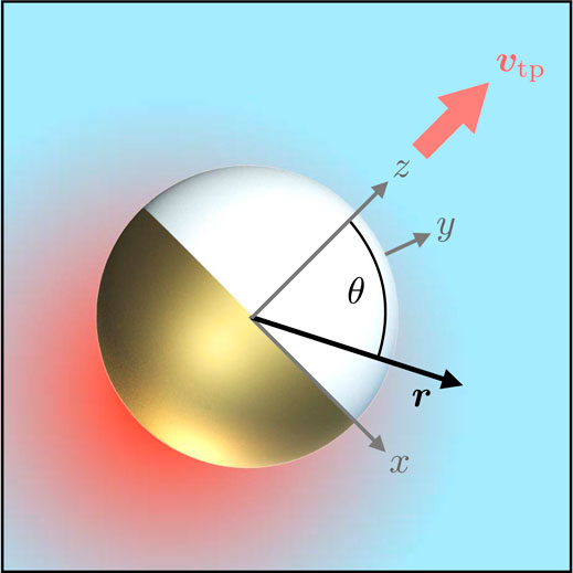
FIGURE 1. Sketch of a spherical Janus particle coated with a thin gold layer on one hemisphere. Upon heating (indicated by the schematic red color gradient), the particle induces an anisotropic temperature profile in the ambient fluid. The resulting thermo-osmotic interfacial flux gives rise to a net propulsion at swim speed vtp along the symmetry axis [2022]. A reference frame attached to the particle’s geometric center has its z-axis aligned with the symmetry axis, pointing towards the uncoated hemisphere. The polar angle between the position vector r and the z-axis is denoted by θ.

Not only does the symmetry breaking complicate the computation of its hot Brownian fluctuations compared to an isotropic particle, it also gives rise to a spontaneous anisotropic solvent flow in its vicinity [23, 24]. Such a particle therefore advances thermophoretically along its symmetry axis, under non-isothermal conditions [20, 21]. In the supplemental material pertaining to this article, we provide evidence that our simulation method indeed leads to a well-controlled, sizable net propulsion of the Janus particle, as was already reported in [22]. Finally, in Sec. 6 we address the largely open task of homogenizing a whole suspension of hot, active particles, before we close with a brief conclusion.

2 Atomistic Model of a Hot Janus Swimmer

Here, we briefly characterize the most salient features of our simulation setup. For additional technical details, the reader is referred to Refs. [22, 2527]. We consider a heated metal-capped Janus sphere immersed in a fluid as depicted in Figure 1. In order to resolve microscopic details, such as the interfacial thermal resistance and the mechanism of thermophoresis [23], our simulation is based on a schematic molecular model, in which both the fluid and the Janus particle are atomistically resolved. All atomic interactions are modeled by a modified Lennard–Jones 12–6 potential

uαβ(r)=4ϵ[(σr)12cαβ(σr)6],(1)

(truncated at r=2.5σ). We henceforth measure length, energies and times in terms of the Lennard–Jones units σ, ϵ, and τmσ2/ϵ, respectively, where m denotes the atomic mass. The solvent molecules always interact via the standard Lennard-Jones potential, i.e., cαβ=css=1. The Janus particle constitutes a spherical cluster of Lennard–Jones atoms additionally bound together by a FENE potential u(r)=0.5ϰR02ln[1(r/R0)2], with the spring constant ϰ=30ϵ/σ2 and R0=1.5σ justified in [28]. The prefactor cαβ in Eq. 1 determines the position (2σ6/cαβ)1/6 of the interaction potential’s minimum. By varying cαβ we can tune the wetting properties of the nanoparticle surface and thereby its Kapitza heat resistance [29, 30]. To mimic the anisotropic physio-chemical properties of Janus spheres, typically realized in experiments [20, 21] by capping one hemisphere of a polystyrene (p) bead with a thin gold (g) layer, we employ the parameters cgs and cps, representing gold-solvent and polystyrene-solvent interactions, respectively. The gold cap is modelled by a 1σ-layer of Lennard–Jones particles on one hemisphere. The wetting parameters cαβ play a significant role in creating the temperature difference across the poles of the Janus particle. At the solid-fluid interface the existence of the interfacial resistance (Kapitza resistance) results in a discontinuity in the temperature profile and this temperature jump is sensitive to the choice of cαβ. Consequently, the temperature jumps across the two surfaces are different, leading to a self-created temperature gradient along the particle axis. Hence, in order to achieve sizeable thermophoretic motion, the imperfect heat conduction between the swimmer’s surface and the adjacent fluid due to the Kapitza heat resistance is important [22]. In our simulations, a periodic cell of length L=50σ was filled with 107,233 solvent molecules, and the Janus sphere, which itself is composed of 767 atoms constituting a particle of radius R5σ. With an integration time step of 0.005τ, our simulations then proceed as follows. At first, the system is equilibrated in the NPT ensemble using a Nose-Hoover thermostat and barostat at a temperature of T0=0.75ϵ/kB and a thermodynamic pressure of p=0.01σ3/ϵ to ensure equilibration of the Lennard-Jones fluid into a liquid state [31, 32]. In the subsequent heating phase, we apply a momentum conserving velocity rescaling procedure to thermostat the gold cap atoms at a temperature TP>T0 while keeping solvent atoms whose distance from the Janus particle is larger than 22σ, at TT0. (We note that other methods to conserve the total energy of similar thermophoretic-microswimmer systems have been employed, e.g., following a dissipative-particle-dynamics approach with energy conservation [33] or combining MD simulation methods with multiparticle collision (MPC) dynamics [34].) The described procedure indeed realizes sizable self-propulsion of the Janus particle [22]. Its propulsion speed and direction are determined by the wetting parameters cαβ of the interaction potential 1) and the heating temperature TP of the gold cap as shown in the supplemental material.

Colloidal thermophoresis has been studied extensively by means of mesoscopic theories and atomistic computer simulations. For example, thermal conductivity and thermodiffusion in nanofluids were studied in [35, 36] by means of nonequilibrium molecular dynamics simulations, whereas Refs. [22, 27, 3739] focused on the realization of self-phoretic microswimmers and the study of their dynamical properties utilizing MPC and/or MD simulation methods. Moreover, molecular simulations were used to quantify thermo-osmotic forces and the associated thermo-osmotic slip [4042], also employing MPC and MD methods. Thermal nonequilibrium transport in colloids and the role of hydrodynamic slip were theoretically studied in [43, 44], and a unified description of colloidal thermophoresis was suggested in [45] using a nonequilibrium-theromodynamics approach. Furthermore, different minimal models have been employed, e.g., to derive a force density from a gradient in a certain potential that is associated with the colloid [4650]. The following paragraphs of the present contribution focus on a specific aspect, which has received relatively little attention so far, namely the enhanced thermal fluctuations experienced by a heated Brownian particle in its (self-created) nonisothermal environment. The swimmer’s so-called hot Brownian motion inevitably interferes with its self-propulsion randomizing particle position and orientation. In the following section, the crucial elementary notion for theories of hot Brownian motion, namely that of a molecular temperature field at which the Lennard–Jones fluid locally equilibrates, is properly introduced, analytically studied, and tested against simulation results.

3 Molecular Temperature Field

In order to justify the concept of a molecular temperature fieldT(r,t), we measured the average kinetic energy of the fluid atoms within 1) thin concentric spherical shells of radial thickness 0.1σ around the particle’s geometric center and 2) angular bins of size π/10 around the Janus sphere. Due to the symmetric particle composition, we expect the temperature profile to depend only on the radial distance r from the particle’s geometric center and the polar angle θ with respect to its symmetry axis. Figure 1 supports these considerations visually. The corresponding angle-averaged and radially averaged temperature profiles, Tθ(r) and Tr(θ), are presented in Figure 2 for various heating temperatures TP of the gold shell. In accordance with previous studies regarding isotropic, homogeneously heated Brownian particles [25, 51, 52], we find the temperature profiles to be stationary, as expected from the strong time scale separation between the swimmer’s motion and the kinetic and energetic equilibration in the solvent. We exploit this fact in Sec. 4 to estimate the effective temperatures governing the particle’s enhanced hot Brownian motion. To get a feeling for the numbers: from the measured compressibility ϰT, viscosity η, fluid density ρ and specific heat cp of the bulk solvent in a thermodynamic state characterized by T0 and p, we obtain DkBT/(6πηR)0.003σ2/τ, DTκ/(ρcp)2σ2/τ and νη/ρ3σ2/τ, for the diffusivities of mass, heat, and vorticity (transverse momentum), respectively [25, 27].

FIGURE 2
www.frontiersin.org

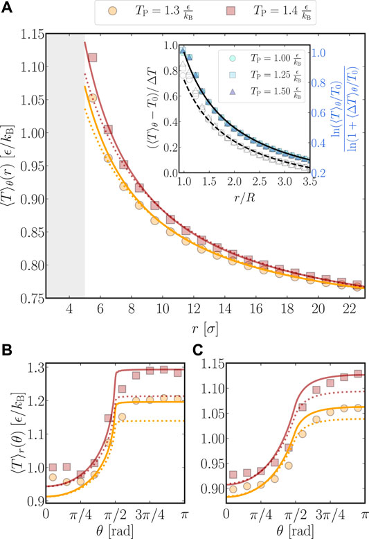
FIGURE 2. Mean fluid temperatures extracted from MD simulations (symbols) with wetting parameters cgs=2 and cps=1 compared to theory (curves). (A) Mean fluid temperature at radius r averaged over concentric spherical shells of thickness 0.1σ for two different heating temperatures TP of the god cap. The Janus spheres’ surface is indicated by the gray bar. Using T0 and ΔT as fit parameters, theory curves are obtained from Eq. 11 (dotted orange/red), and by θ-averaging the dipole approximation of Eq. 13 (solid orange/red). Inset: Data collapse for three distinct heating powers, characterized by the particle temperatures given in the legend. The reduced temperature fields are obtained according to the l.h.s. of Eq. 16/Eq. 15 using fit parameters (T0,ΔT) / (T0,ΔTθ) as obtained in the main plot, open/filled symbols referring to the left/right y-axis. Black solid and dashed lines represent a R/r and B0R/r decay, respectively, with B0=1/2+1/π, Eq. 7. (B), (C) The measured radially averaged fluid temperature as a function of the polar angle for two distinct heating temperatures [same as in (A)], averaged up to a distance of 0.1σ and 2.5σ from the surface, respectively. For the dotted theory curves we radially averaged the first 100 terms of Eq. 6, while the solid lines were obtained from the first 100 terms of the numerically averaged profile in (13); parameters T0, ΔT as obtained in (A).

We start our quantitative discussion with the thermodynamic description of heat conduction. In steady state, the heat conduction equation for the temperature profile T(r) reads [53].

Q(r)=[κ(r)T(r)](2)
=κ(r)T(r)+κ(r)2T(r),(3)

where κ(r) denotes the heat conductivity and Q(r) is the heat flux absorbed by the gold cap. Equation 3 is accompanied by boundary conditions at the particle surface r=R. In our simulations, a sudden temperature drop at the particle-fluid interface signifies a substantial Kapitza heat resistance. In the simplified theory, we neglect this effect and enforce the continuity of the temperature profiles inside and outside the particle, Tin(R,θ)=Tout(R,θ), for the sake of simplicity. Following the derivations in [24], we also demand continuity in the normal component of the heat flux,

κinrTin=κoutrToutfor0θπ/2,(4)

along the uncoated part of the Janus sphere. Motivated by its very large heat conductivity, the gold cap of the Janus sphere is modelled as an isotherm kept at surface temperature

T(R,θ)=T0+ΔTforπ/2θπ,(5)

where ΔT denotes the increment relative to the ambient temperature T0 of the fluid. We further set the heat conductivities κin=κoutκ for the remainder of this section. Besides, we henceforth omit the subscript for the outer temperature profile, ToutT, as the temperature profile inside the particle is not relevant in the following. If, as a first crude approximation, we finally assume that κ=const. throughout the whole system, the temperature field T(r,θ) is given by [24].

T(r,θ)=T0+ΔTn=0BnPn(cosθ)(Rr)n+1,(6)

with the Legendre polynomials Pn and expansion coefficients

B0=12+1π,B2k=B2k+1=1π(1)k2k+1.(7)

Due to the orthogonality relations (δlk denotes the Kronecker-delta)

11dc Pk(c)Pl(c)=22l+1δkl,(8)

and with the short-hand notation ccosθ, the angle-averaged temperature profile Tθ(r) simplifies to

T0+ΔTθ(r)=0πdθT(r,θ)sinθ0πdθsinθ=11dcT(r,c)11dc,(9)
=T0+ΔT2n=0Rn+1rn+111dcBnPn(c),(10)
=T0+ΔTB0Rr.(11)

We infer from Eq. 11 that the actual and mean surface temperature increment are related via

B0=ΔTθΔT.(12)

Using the ambient fluid temperature T0 and the surface increment ΔT as parameters, we fitted Eq. 11 to the numerically simulated average temperature profiles. The resulting fits are presented in Figure 2A for two distinct heating temperatures (dotted curves). Matching the measured temperature profiles well at larger distances, the theory curves slightly but systematically underestimate the numerical data closer to the particle surface. As a result, the mean surface temperature increment ΔTθ and thus, viaEq. 12, also ΔT itself, are underestimated. This becomes even more pronounced when comparing measurements of the radially averaged temperature data Tr(θ) to the corresponding radial average of the theory curve 6) as shown in Figures 2B,C. The former plot depicts Tr(θ) close to the particle surface, whereas for the latter one, we averaged up to a distance 2.5σ away from the swimmer’s surface. In both cases the dotted theory curves lie significantly below the numerical data, especially on the coated part (π/2θπ) of the particle.

The described shortcomings of the theoretical temperature profile 6) can be improved by taking the temperature dependence of the heat conductivity κ(T) of the fluid into account. For the studied Lennard–Jones fluid, the heat conductivity approximately follows a (T1)-law [25]. Plugging κ1/T into Eq. 3, the ansatz T(r,θ)=T0exp[ψ(r,θ)] yields the equation 2ψ(r,θ)Q(r,θ) for the auxiliary dimensionless field ψ(r,θ). Sticking to thick-cap boundary conditions, 4) and (5), ψ(r,θ) solves the same boundary value problem as the temperature field in the previously discussed case of κ=const., albeit the latter boundary condition now reads ψ(R,θ)=ln(1+ΔT/T0) for π/2θπ. Hence, the solution for ψ(r,θ) equals the one given in Eq. 6 upon replacing T00 and ΔTln(1+ΔT/T0). The resulting temperature field eventually takes the form

Tκ(r,θ)=T0(1+ΔTT0)n=0BnPn(cosθ)(Rr)n+1.(13)

As detailed in the supplemental material, an analytic expression for the radially averaged temperature field Tκθ(r) can be calculated when truncating the infinite series in the exponent of Eq. 13 after n=1 (dipole) or n=2 (quadrupole). The solid curves in Figure 2A corresponds to the averaged dipole approximation, which represents the simulation data very well, also close to the particle surface. The quadrupole approximation is practically indistinguishable from it and is therefore not depicted in Figure 2A. Remarkably, also the temperature field [25].

Tθ(r)=Thom(r)=T0(1+ΔTθT0)R/r(14)

of an isotropic particle homogeneously heated up by ΔTθ delivers great fits to the data. Here, ΔTθ served as a fit parameter. Since the corresponding fits to the temperature profiles would be indistinguishable from the solid curves, the superiority of Eq. 14 over the κ=const. approximation, Eq. 11, is illustrated in the inset of Figure 2A. The colored symbols and the solid line show that measured average temperature profiles Tθ for distinct heating temperatures nicely collapse onto the prediction

ln(Tθ/T0)ln(1+ΔTθ/T0)=Rr(15)

obtained by rearranging Eq. 14. In contrast, the collapse is violated close to the particle surface when the temperature profiles are simplified according to Eq. 11,

TθT0ΔT=B0Rr,(16)

as can be inferred from the open symbols and dashed curve. This indicates that, close to the particle surface, the characteristic decay of Tθ(r) is significantly influenced by the temperature dependence of the heat conductivity κ(T), whereas heterogeneities in the particle-fluid interactions can be subsumed into a single (fit-)parameter ΔTθ. In order to resolve the angle dependence of the temperature profile, we have to resort back to Eq. 13. Using the obtained optimal fit parameters for T0 and ΔT, we numerically determined the angle-resolved temperature profiles Tκr(θ). They improve the quantitative agreement with the simulation data, as the solid curves in Figures 2B,C indicate. Moreover, the theory curves in both panels are free of spurious fluctuations that were present in previous attempts to fit the angle-resolved temperature profiles [22].

The measured temperature profiles in Figure 2B also show that for θπ/2, the metal cap is not well described by an isotherm. Thus, our theoretical prediction slightly overestimates the temperature profile in those regions. Also, close to the pole of the particle’s uncoated hemisphere (θ0) the measurements indicate a slight temperature increase—an effect that fades further away from the particle surface as Figure 2C shows. The investigation of this effect bears potential for future studies as it might indicate a feedback of the particle’s hydrodynamic flow field [24] onto the temperature profile. Further improvement of the fits might be obtained by taking the numerically observed Kapitza heat resistance into account.

Having justified the notion of a local molecular temperature, we next exploit the aforementioned Brownian time scale separation in order to calculate the effective nonequilibrium temperatures THBM that characterize the Janus particle’s overdamped hot Brownian motion.

4 Hot Brownian Motion

A hot nanoswimmer is inevitably subject to Brownian motion which randomizes the path of the particle in both position and orientation. In the classical Langevin picture of equilibrium Brownian motion, the Sutherland-Einstein relation

D=kBT0/ζ(17)

for the particle diffusivity D guarantees that the stochastic forces driving the Brownian particle balance the losses by the friction ζV, with friction coefficient ζ and velocity V, such as to maintain the Gibbs equilibrium at the temperature T0. Equation 17 links the atomistic world, represented by the Boltzmann constant kB, to mesoscopic transport coefficients, D and ζ. The existence of such a fluctuation-dissipation relation is often taken for granted even when there are temperature gradients present in the solvent, as is the case for heated nanoparticles. In this situation, however, the stochastic force on the particle must be evaluated as the superposition of the thermal fluctuations within the whole solvent. In the Markov limit, i.e., on time scales where the particle’s momentum and hydrodynamic modes have fully relaxed and Brownian fluctuations are effectively diffusive [26], generalized overdamped Langevin equations of the form

0=(M00I)(V˙Ω˙)=Z(VΩ)+ξ(t)+(FextText)(18)

are found to hold [54, 55]. Here, M,I denote the particle’s mass and tensor of inertia, V,Ω its translational and rotational velocity, Z the 6×6 friction tensor, ξ(t) Gaussian white noise, and Fext,Text the external force and torque, respectively. The equations of motion are complemented by the specification of the noise strength

ξ(t)=0,(19)
ξμ(t)ξν(t)THBMμνZHBMμνδ(tt),(20)

with effective temperatures THBMμν and friction coefficients ZHBMμν, respectively. The superscript μν indicates that for non-isothermal Brownian motion, different degrees of freedom (e.g., translation, rotation, or both coupled) sense distinct effective temperatures [55] rendering THBM, in general, a tensorial quantity. Using the framework of fluctuating hydrodynamics, the effective temperatures THBMμν turn out to be given by a weighted spatial average of the local solvent temperature field T(r) [54]:

THBMμν=drT(r)ϕμν(r)drϕμν(r).(21)

The weight function

ϕμν(r)η(r)i,j[iujμ(r)iujν(r)+iujν(r)juiμ(r)](22)

is the (excess) viscous dissipation function induced by the velocity fields uμ,ν pertaining to the considered motion and η is the dynamic viscosity of the fluid. Note that THBMμν is therefore a tensorial quantity.

We stress the fact that the theory of hot Brownian motion connects the particle’s enhanced thermal fluctuations with the associated energy dissipation into the ambient fluid. Therefore, the dissipation function ϕμν defined in Eq. 22 must not include contributions due to the particle’s active swimming, even though the latter typically exceeds the former considerably.

In the following section, we use Eq. 21 to estimate effective temperatures characterizing the rotational and translational hot Brownian motion of a Janus sphere.

5 Estimating THBM for a Janus Sphere

Since a generally temperature dependent viscosity η(T) renders the calculation of effective temperatures rather complicated, we pursue a similar approach as in [51, 52], where a first estimate for THBMμν could be obtained by employing a temperature independent viscosity ηη0. In the case of a homogeneously heated particle [51, 52] with a surface temperature increment ΔT, this lead to the first order term in THBM(ΔT). Following the same route, we calculate the effective temperatures THBMθ/ and THBMx/ for a Janus sphere. The superscripts represent motion types considered in this article, namely.

θ/: rotation about/perpendicular to the particle’s symmetry axis,

x/: translation along/transverse to the symmetry axis.

The effective temperature THBMm corresponding to the considered motion type m{θ/,x/} is given by

THBMm=drT(r)ϕm(r)drϕm(r)(23)

Note that superpositions of the motion types listed above generally sense yet different effective temperatures, e.g., THBMx,θ. Here, we only consider the elementary degrees of freedom.

The temperature field around a Janus sphere of radius R solves the heat conduction Eq. 3. Assuming constant viscosity and heat conductivity κ, the solution can be expanded in terms of Legendre polynomials Pn as

T(r,θ)=T0+n=0TnPn(cosθ)(Rr)n+1,(24)

with the ambient fluid temperature T0. The expansion coefficients Tn are determined by boundary conditions at the particle surface, which we do not further specify here. Analogous to the calculation in Eqs 911, the average surface temperature increment is given by

ΔTθ=T0.(25)

Since the coefficient T0 pertains to an angle independent 1/r-decay in the temperature field (24), it represents a spherical particle homogeneously heated to T0+ΔTθ. Higher coefficients Tn>0 characterize anisotropies of the temperature field.

We now turn to the calculation of the effective temperature THBMxviaEq. 23, where we first consider the Janus particle’s translation along its symmetry axis. Introducing the abbreviations ssinθ and ccosθ, the corresponding viscous dissipation function for a sphere of radius R at translation speed V within an infinite homogeneous system with constant viscosity reads [52].

ϕx(r,θ)=η0[fs(r)s2+fc(r)c2],(26)

where we introduced

fs(r)9r8K22,(27)
fc(r)3r8(K1r2+3K2)2,(28)

with the constant coefficients K1=3VR/2 and K2=VR3/2. As the dissipation function ϕx is composed of terms proportional to s2 and c2=1s2, the product of T(r,θ) and ϕx(r,θ) in the enumerator of Eq. 23 yields integrals over the polar angle of the kind 11dcs2Pn(c). By virtue of the relation s2=2[P0(c)P2(c)]/3 and Eq. 8, this integral simplifies to

11dcs2Pn(c)=23(2δ0n2n+12δ2n2n+1).(29)

Therefore, only the coefficients T0 and T2 from the infinite series 24) contribute to THBMx, while all other terms vanish by symmetry upon averaging, which actually holds for all cases considered in this article. Explicit calculation of THBMxviaEq. 23 gives for the non-trivial part of the numerator:

2T0Rdrr2fs(r)Rr(30)
+23T0Rdrr2[fc(r)fs(r)]Rr(31)
+415T2Rdrr2[fc(r)fs(r)](Rr)3(32)
=34T0RV2+12T0RV2+0(33)
=54T0RV2.(34)

The denominator analogously gives 3RV2. With Eq. 25, we finally obtain

THBMx=T0+512ΔTθ.(35)

Hence, for translation along its symmetry axis, the Janus sphere’s hot Brownian motion is identical to that of a sphere homogeneously heated by ΔTθ [52]. The vanishing integral in line 32) reveals that there is no coupling between the dissipation function ϕx and angular variations in the temperature field represented by T2. Therefore, no correction term accompanies the factor 5/12 in THBMx. This result could have been anticipated as the authors of Ref. [54] showed that a linear temperature field implies no corrections to the standard Langevin description of Brownian motion when the viscosity is assumed to be constant.

As anticipated on the same grounds and explicitly shown in the supplemental material, a similar calculation with a simple coordinate transformation leads to

THBMx=T0+512ΔTθ,(36)

for the particle’s translation perpendicular to its symmetry axis. Thus, also for transverse motion the corresponding effective temperatures are exactly given by those of a sphere homogeneously heated up by ΔTθ.

We now turn to the particle’s rotational degrees of freedom starting with the calculation of THBMθ for rotation about its symmetry axis. The corresponding viscous dissipation function for a rotating sphere reads [51].

ϕθ(r,θ)r6sin2θ.(37)

Using Eq. 29, the non-trivial part of the numerator of Eq. 23 evaluates to

23n=0Rdr11dcPn(c)1r4(Rr)n+1[P0(c)P2(c)](38)
=23[2T0RdrRr525T2RdrR3r7](39)
=49R3[34T0110T2],(40)

and likewise the denominator to

43Rdrr4=49R3.(41)

Using T0=ΔTθ finally yields

THBMθ=T0+ΔTθ(34110T2ΔTθ).(42)

In contrast to our results for translation, Eq. 35, Eq. 36, we find that THBMθT0 is composed of two parts: 1) the contribution 3ΔTθ/4 corresponding to an isotropic sphere homogeneously heated up by ΔTθ [51] and 2) a correction term proportional to T2. The latter stems from a non-vanishing coupling between the θ-dependence of the temperature field 24) and the dissipation function (37). For most practical cases, the correction term is negligible with respect to 3/4 since, typically, T2<T0=ΔTθ. For instance, in the thick-cap limit, for which the temperature field is explicitly given by Eq. 6, Eq. 7, one has. T2/(10T0)0.03.

A simple coordinate transformation (see supplemental material) and similar calculations as presented above yield

THBMθ=T0+ΔTθ(34+120T2ΔTθ),(43)

for rotation perpendicular to the particle’s symmetry axis. In this case, the correction term is only half in magnitude and has opposite sign as compared to the one in Eq. 42. This stems from the fact that the symmetry axis of the particle, and thus of the temperature profile, does not coincide with the rotation axis, thus leading to a distinct coupling between the temperature field and the dissipation function.

In order to test the theory, we measured the effective temperatures using MD computer simulations as described in Sec. 2. We therefor additionally confined the Janus sphere employing an external angular or spatial harmonic potential parallel or perpendicular to its symmetry axis [51] and measured its response. Figures 3A,B illustrate the respective distributions of the Janus particle’s position z and orientation θ relative to its symmetry axis for distinct heating temperatures.

FIGURE 3
www.frontiersin.org

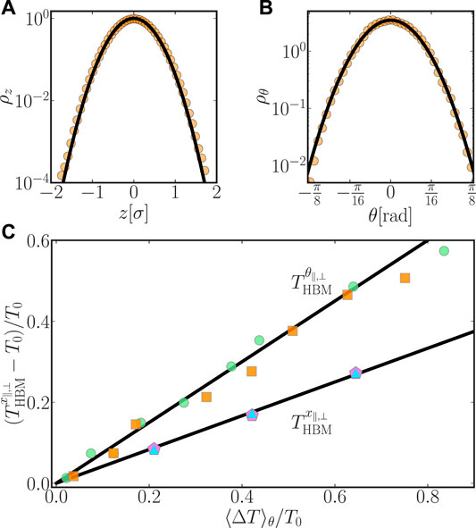
FIGURE 3. Upper panels: Histograms of harmonically confined position (A) and orientation (B) of the Janus particle heated to TP=1.0ϵ/kB in (A) and TP=1.0ϵ/kB in (B). Histograms were fitted by Gaussian profiles (lines) to extract the corresponding effective temperature THBM. (C) Lower line and data: Numerically measured THBMx (blue triangles), THBMx (pink pentagons) for translation along/transverse to the symmetry axis of a heated Janus particle against the theory from Eq. 35, Eq. 36. Upper line and data: THBMθ (orange squares) for rotation around the particle’s symmetry axis, and THBMθ for an isotropic, homogeneously heated Brownian particle [51] (green circles) versus theory from Eq. 42, neglecting the small correction term (which would hardly be discernible, anyway). In all simulations, the wetting parameters were cps=1 and cgs=2.

From the variances of the effectively Gaussian distributions, we extracted the effective temperatures for translation and rotation, respectively [51]. The corresponding average surface temperature increments ΔTθ were obtained by fitting the angle averaged temperature profiles viaEq. 14 (cf. Figure 2). As Figure 3C shows, the measured effective temperatures are nicely described by our theory. We also compared our results to the effective temperatures for a homogeneously heated Brownian particle. The prediction for the enhanced diffusion of homogeneous hot Brownian spheres has been quantitatively verified in dedicated experiments [56, 57]. According to the theory, a similar enhancement of the long-time diffusivity must be expected for the transverse and rotational motion of a Janus sphere. Along the particle’s axis of propulsion, the long-time diffusivity is typically dominated by its active propulsion [26].

Having seen that the coarse-grained non-equilibrium hydrodynamic description works well on the single-particle level, we now address the task of further coarse graining a suspension of hot microswimmers to an effective homogeneous complex fluid. Although for related microswimmer systems, scientists have developed powerful methods accounting for large numbers of individual swimmers [5861], the task of homogenizing a whole suspension of hot, active particles and the role of effective nonequilibrium temperatures has received relatively little attention.

6 Complex Fluid Homogenisation

One is often interested in the collective (thermo) dynamical properties of an assembly of colloids and their embedding solvent, rather than in the motion of a single unit. Particle-based descriptions are impractical to inspect the behavior of such a complex fluid and one therefore often seeks a more versatile continuum approach, which allows one to leapfrog, in an efficient way, over the diverse time and length scales of its various constituents.

To this aim, we study non-isothermal fluctuating hydrodynamic equations of a fluid with suspended colloids, which are recast in terms of dynamical equations for coarse-grained volume elements. Surprisingly, a non-local frequency-dependent temperature appears due to the presence of the dispersed particles, which characterizes the intensity of their thermal fluctuations. Consider an incompressible solvent of density ϱ with velocity field u described by the linearized fluctuating hydrodynamic equations [55].

ϱtu(r,t)=σ(r,t)+τ(r,t),(44)

and N suspended colloids coupled to the fluid velocity via no-slip boundary conditions. Here, σ denotes the total stress tensor and τ is a zero-mean Gaussian random stress tensor with delta correlations in space and time. The molecular temperature is prescribed by the heat equations. For later convenience, we assume that the flow field u is defined also inside the colloids, where it equals identically the colloid velocity Vi, namely

u(r,t)=Vi,if |rXi|<R.(45)

The colloids are idealized as spheres with radius R and mass M, and their positions are denoted by Xi.

The coarse-graining procedure proceeds as follows:

1. We divide the system into mesoscopic volumes V(r), with edge length l, located at position r. Old and new coordinates, r and r respectively, are related by the scaling r=r/l, where l defines the coarse-graining length scale, much larger than the colloidal radius R.

2. We define the coarse-grained velocity of the complex fluid U(r,t) as the spatial average over the coarse-grained volume ν(r)

U(r,t)=1l3ν(r)dru(r,t).(46)

3. In Eq. 46 the integration volume ν(r) is split into the volume occupied by the solvent νs(r) and that occupied by the solute particles νp(r). Introducing the local particle volume fraction ϕ(r)|νp(r)|/|ν(r)|, we obtain

U(r,t)=1l3νs(r)dru(r,t)+ϕ(r)V¯(r,t),(47)

where we have defined the local average velocity of the colloids

V¯(r,t)1N(r)iν(r)Vi(t),(48)
N(r)iν(r)1.(49)

4. We take the time derivative of Eq. 47,

tU(r,t)=1l3vs(r)drtu(r,t)+ϕ(r)tV¯(r,t).(50)

The first summand is rewritten, using Eq. 44

1l3νs(r)drtu(r,t)(51)
=1ϱl3vs(r)dr(σ(r,t)+τ(r,t))(52)
=1ϱ(σ˜(r,t)+τ˜(r,t)),(53)

where σ˜ and τ˜ are the coarse-grained stress tensors.

It is not hard to convince oneself that the random tensor τν is still a zero-mean Gaussian noise with delta correlations in space and time. In fact, using the divergence theorem the mean is

νs(r)d2rnτ(r,t)=0,(54)

and the correlation function becomes

νs(r1)d2rνs(r2)d2rnnτ(r,t)τ(r,t)=2νs(r1)d2rνs(r2)d2rnnη(r)T(r)δ(rr)δ(tt),(55)

which is nonzero only if r1=r2 and is proportional to δ(tt). Here, n and n denotes the inner normal vectors along the surface vs(r1,2) of the respective volume element. For the second summand in Eq. 50, we decompose the particle velocity Vi(t)=vtp,i(t)+V˜i(t) into thermophoretic propulsion (induced by the deterministic local temperature field) and nonisothermal fluctuations (induced by the ambient fluid’s thermal fluctuations [54]). Assuming that the suspension of hot microswimmers is sufficiently dilute so that hydrodynamic and temperature-mediated interactions between the colloids are negligible, each particle (approximately) propels at a constant speed v0 along its current orientation n^i(t). For common experimental conditions this ballistic motion dominates over its diffusive transport, at late times, but remains slow compared to the fluid response [26]. Then, the second summand in Eq. 50 is [54].

ϕ(r)N(r)iν(r)Vi(t)=ϕ(r)N(r)iν(r)(ν0Ω˜i(t)×n^i(t)tdtZx(Xi,tt)V˜i(t)M+ξix(Xi,t)),(56)

where, we used n^˙i(t)=Ω˜i(t)×n^i(t), with the particle’s angular velocity Ω˜i(t), and introduced the time-dependent friction kernel Zx(Xi,t) and the unbiased white Gaussian noise process ξix(Xi,t) corresponding to particle translation. Since interactions between colloids are neglected (dilute-solution approximation), the angular velocity is solely governed by the fluctuating hydrodynamics of the medium and obeys generalized Langevin equations of the form [54, 55].

IΩ˜˙i(t)=tdtZθ(Xi,tt)Ω˜i(t)+ξiθ(Xi,t),(57)

where we introduced the particle moment of inertia I, and the time-dependent rotational friction kernel Zθ(Xi,t) and the unbiased white Gaussian noise process ξiθ(Xi,t) for the particle rotation. Therefore, the average acceleration is given by a sum of generalized Langevin equations of the type previously derived for hot Brownian motion [54, 55]. We use the result obtained for a generic (but stationary) temperature field T(r), here generated by the colloids sitting in their average positions. The noise spectrum reads

ξiμ(Xi,ω)ξiν(Xi,ω)Tμν(Xi,ω)Zμν(Xi,ω)(58)

and displays a tensorial frequency-dependent temperature—generally distinct from T(r)

Tμν(Xi,ω)Vd3rϕμν(r,ω)T(Xi+r)Vd3rϕμν(r,ω),(59)

whose zero-frequency limit should be compared with Eq. 21. The weight function ϕμν(r,ω) denotes the (excess) viscous dissipation function associated to the unsteady thermal motion of a colloid. For this to apply to all particles in the suspension, the latter has to be sufficiently dilute so that hydrodynamic and temperature-mediated interactions between the colloids are negligible. Under this assumption, also thermal noises acting on different colloids can be taken to be uncorrelated.

This analysis suggests that a non-trivial coarse-grained noise temperature arises through the presence of “slow” degrees of freedom. These are, in a hydrodynamic description, coupled to the fast ones via boundary conditions and thus are subjected to long-range forces, in contrast to the local, Markovian thermal stresses acting on the fluid elements.

7 Conclusion

We have performed microscopically resolved molecular dynamics simulations of a single hot Janus swimmer immersed in a Lennard-Jones fluid. We locally measured the inhomogeneous and anisotropic temperature profile induced in the solvent and compared it against analytic expressions basing on the heat conduction equation. We thereby verify the notion of a molecular temperature at which the surrounding medium locally equilibrates. We then exploited a large Brownian timescale separation in order to address the Janus particle’s overdamped hot Brownian motion. In a first-order approximation in the mean temperature increment ΔTθ of the particle surface, we calculate effective nonequilibrium temperatures THBM for distinct types of motion. Our theoretical predictions nicely agree with measurements of THBM over a wide temperature range. In the last coarse-graining step, we studied non-isothermal fluctuating hydrodynamic equations of a fluid with such suspended nonisothermal active colloids. The noise spectrum of the coarse-grained fluid is governed by tensorial, local and frequency-dependent effective temperatures that generally differ from the local molecular temperature field in the solvent. They have to separately be taken along in any attempt to coarse grain a suspension of hot particles into a an effectively homogeneous complex fluid.

Data Availability Statement

The original contributions presented in the study are included in the article/Supplementary Material, further inquiries can be directed to the corresponding authors.

Author Contributions

The simulations were designed and performed by DC and RP. Both also analyzed the raw data. The theory was done by SA and GF. The manuscript was written by SA and KK.

Funding

We acknowledge funding by the Deutsche Forschungsgemeinschaft (DFG) through the priority program “Microswimmers” (SPP 1726, project 237143019), and Leipzig University within the program of Open Access Publishing. This work was supported by funding from the Science and Engineering Research Board (SERB), India, vide Grant No. SB/S2/CMP-113/2013 and by nVidia® corporation through its GPU Grant Program.

Conflict of Interest

The authors declare that the research was conducted in the absence of any commercial or financial relationships that could be construed as a potential conflict of interest.

Supplementary Material

The Supplementary Material for this article can be found online at: https://www.frontiersin.org/articles/10.3389/fphy.2021.655838/full#supplementary-material

References

1. Aharony A, Entin-Wohlman O. Perspectives of Mesoscopic Physics: Dedicated to Yoseph Imry’s 70th Birthday. London: World Scientific Publishing Company (2010).

2. Kroy K, Frey E. Focus on Soft Mesoscopics: Physics for Biology at a Mesoscopic Scale. New J Phys (2015) 17:110203. doi:10.1088/1367-2630/17/11/110203

CrossRef Full Text | Google Scholar

3. Laughlin RB, Pines D. The Theory of Everything. Proc Natl Acad Sci (2000) 97:28–31. doi:10.1073/pnas.97.1.28

PubMed Abstract | CrossRef Full Text | Google Scholar

4. Gompper G, Ihle T, Kroll DM, Winkler RG. Multi-particle Collision Dynamics: A Particle-Based Mesoscale Simulation Approach to the Hydrodynamics of Complex Fluids. Adv Comp Simulation Approaches Soft Matter Sci (2009) III:1–87. doi:10.1007/978-3-540-87706-6_1

CrossRef Full Text | Google Scholar

5. Carenza LN, Gonnella G, Lamura A, Negro G, Tiribocchi A. Lattice Boltzmann Methods and Active Fluids. Eur Phys J E (2019) 42:81. doi:10.1140/epje/i2019-11843-6

PubMed Abstract | CrossRef Full Text | Google Scholar

6. Shaebani MR, Wysocki A, Winkler RG, Gompper G, Rieger H. Computational Models for Active Matter. Nat Rev Phys (2020) 2:181–99. doi:10.1038/s42254-020-0152-1

CrossRef Full Text | Google Scholar

7. Steffenoni S, Kroy K, Falasco G. Interacting Brownian Dynamics in a Nonequilibrium Particle bath. Phys Rev E (2016) 94:062139. doi:10.1103/PhysRevE.94.062139

PubMed Abstract | CrossRef Full Text | Google Scholar

8. Lämmel M, Kroy K. Analytical Mesoscale Modeling of Aeolian Sand Transport. Phys Rev E (2017) 96:052906. doi:10.1103/PhysRevE.96.052906

PubMed Abstract | CrossRef Full Text | Google Scholar

9. Bregulla AP, Yang H, Cichos F. Stochastic Localization of Microswimmers by Photon Nudging. ACS Nano (2014) 8:6542–50. doi:10.1021/nn501568e

PubMed Abstract | CrossRef Full Text | Google Scholar

10. Jikeli JF, Alvarez L, Friedrich BM, Wilson LG, Pascal R, Colin R, et al. Sperm Navigation along Helical Paths in 3d Chemoattractant Landscapes. Nat Commun (2015) 6:7985. doi:10.1038/ncomms8985

PubMed Abstract | CrossRef Full Text | Google Scholar

11. Qian B, Montiel D, Bregulla A, Cichos F, Yang H. Harnessing thermal Fluctuations for Purposeful Activities: the Manipulation of Single Micro-swimmers by Adaptive Photon Nudging. Chem Sci (2013) 4:1420–9. doi:10.1039/c2sc21263c

CrossRef Full Text | Google Scholar

12. Selmke M, Khadka U, Bregulla AP, Cichos F, Yang H. Theory for Controlling Individual Self-Propelled Micro-swimmers by Photon Nudging I: Directed Transport. Phys Chem Chem Phys (2018) 20:10502–20. doi:10.1039/c7cp06559k

PubMed Abstract | CrossRef Full Text | Google Scholar

13. Selmke M, Khadka U, Bregulla AP, Cichos F, Yang H. Theory for Controlling Individual Self-Propelled Micro-swimmers by Photon Nudging II: Confinement. Phys Chem Chem Phys (2018) 20:10521–32. doi:10.1039/c7cp06560d

PubMed Abstract | CrossRef Full Text | Google Scholar

14. Adhikari R, Stratford K, Cates ME, Wagner AJ. Fluctuating Lattice Boltzmann. Europhys Lett (2005) 71:473–9. doi:10.1209/epl/i2004-10542-5

CrossRef Full Text | Google Scholar

15. Menon GI. Active Matter. Rheology of Complex Fluids (2010) 1:193–218. doi:10.1007/978-1-4419-6494-6_9

CrossRef Full Text | Google Scholar

16. Marchetti MC, Joanny JF, Ramaswamy S, Liverpool TB, Prost J, Rao M, et al. Hydrodynamics of Soft Active Matter. Rev Mod Phys (2013) 85:1143–89. doi:10.1103/revmodphys.85.1143

CrossRef Full Text | Google Scholar

17. Celani A, Bo S, Eichhorn R, Aurell E. Anomalous Thermodynamics at the Microscale. Phys Rev Lett (2012) 109:260603. doi:10.1103/physrevlett.109.260603

PubMed Abstract | CrossRef Full Text | Google Scholar

18. Seifert U. Stochastic Thermodynamics, Fluctuation Theorems and Molecular Machines. Rep Prog Phys (2012) 75:126001. doi:10.1088/0034-4885/75/12/126001

PubMed Abstract | CrossRef Full Text | Google Scholar

19. Braun M, Cichos F. Optically Controlled Thermophoretic Trapping of Single Nano-Objects. ACS Nano (2013) 7:11200–8. doi:10.1021/nn404980k

PubMed Abstract | CrossRef Full Text | Google Scholar

20. Jiang H-R, Yoshinaga N, Sano M. Active Motion of a Janus Particle by Self-Thermophoresis in a Defocused Laser Beam. Phys Rev Lett (2010) 105:268302. doi:10.1103/physrevlett.105.268302

PubMed Abstract | CrossRef Full Text | Google Scholar

21. Bregulla AP, Cichos F. Size Dependent Efficiency of Photophoretic Swimmers. Faraday Discuss (2015) 184:381–91. doi:10.1039/c5fd00111k

PubMed Abstract | CrossRef Full Text | Google Scholar

22. Kroy K, Chakraborty D, Cichos F. Hot Microswimmers. Eur Phys J Spec Top (2016) 225:2207–25. doi:10.1140/epjst/e2016-60098-6

CrossRef Full Text | Google Scholar

23. Anderson JL. Colloid Transport by Interfacial Forces. Annu Rev Fluid Mech (1989) 21:61–99. doi:10.1146/annurev.fl.21.010189.000425

CrossRef Full Text | Google Scholar

24. Bickel T, Majee A, Würger A. Flow Pattern in the Vicinity of Self-Propelling Hot Janus Particles. Phys Rev E Stat Nonlin Soft Matter Phys (2013) 88:012301. doi:10.1103/PhysRevE.88.012301

PubMed Abstract | CrossRef Full Text | Google Scholar

25. Chakraborty D, Gnann MV, Rings D, Glaser J, Otto F, Cichos F, et al. Generalised Einstein Relation for Hot Brownian Motion. Epl (2011) 96:60009. doi:10.1209/0295-5075/96/60009

CrossRef Full Text | Google Scholar

26. Falasco G, Pfaller R, Bregulla AP, Cichos F, Kroy K. Exact Symmetries in the Velocity Fluctuations of a Hot Brownian Swimmer. Phys Rev E (2016) 94:030602(R). doi:10.1103/PhysRevE.94.030602

PubMed Abstract | CrossRef Full Text | Google Scholar

27. Chakraborty D. Orientational Dynamics of a Heated Janus Particle. J Chem Phys (2018) 149:174907. doi:10.1063/1.5046059

PubMed Abstract | CrossRef Full Text | Google Scholar

28. Grest GS, Kremer K. Molecular Dynamics Simulation for Polymers in the Presence of a Heat bath. Phys Rev A (1986) 33:3628–31. doi:10.1103/physreva.33.3628

CrossRef Full Text | Google Scholar

29. Barrat J-L, Bocquet Lr.. Influence of Wetting Properties on Hydrodynamic Boundary Conditions at a Fluid/solid Interface. Faraday Disc. (1999) 112:119–28. doi:10.1039/a809733j

CrossRef Full Text | Google Scholar

30. Barrat J-L, Chiaruttini F. Kapitza Resistance at the Liquid-Solid Interface. Mol Phys (2003) 101:1605–10. doi:10.1080/0026897031000068578

CrossRef Full Text | Google Scholar

31. Errington JR, Debenedetti PG, Torquato S. Quantification of Order in the Lennard-Jones System. J Chem Phys (2003) 118:2256–63. doi:10.1063/1.1532344

CrossRef Full Text | Google Scholar

32. Potoff JJ, Panagiotopoulos AZ. Critical point and Phase Behavior of the Pure Fluid and a Lennard-jones Mixture. J Chem Phys (1998) 109:10914–20. doi:10.1063/1.477787

CrossRef Full Text | Google Scholar

33. Fedosov DA, Sengupta A, Gompper G. Effect of Fluid-Colloid Interactions on the Mobility of a Thermophoretic Microswimmer in Non-ideal Fluids. Soft Matter (2015) 11:6703–15. doi:10.1039/c5sm01364j

PubMed Abstract | CrossRef Full Text | Google Scholar

34. Yang M, Ripoll M. Simulations of Thermophoretic Nanoswimmers. Phys Rev E Stat Nonlin Soft Matter Phys (2011) 84:061401. doi:10.1103/PhysRevE.84.061401

PubMed Abstract | CrossRef Full Text | Google Scholar

35. Vladkov M, Barrat J-L. Modeling Transient Absorption and thermal Conductivity in a Simple Nanofluid. Nano Lett (2006) 6:1224–8. doi:10.1021/nl060670o

PubMed Abstract | CrossRef Full Text | Google Scholar

36. Galliero G, Volz S. Thermodiffusion in Model Nanofluids by Molecular Dynamics Simulations. J Chem Phys (2008) 128:064505. doi:10.1063/1.2834545

PubMed Abstract | CrossRef Full Text | Google Scholar

37. Lüsebrink D, Yang M, Ripoll M. Thermophoresis of Colloids by Mesoscale Simulations. J Phys Condens Matter (2012) 24:284132. doi:10.1088/0953-8984/24/28/284132

PubMed Abstract | CrossRef Full Text | Google Scholar

38. Yang M, Wysocki A, Ripoll M. Hydrodynamic Simulations of Self-Phoretic Microswimmers. Soft Matter (2014) 10:6208–18. doi:10.1039/c4sm00621f

PubMed Abstract | CrossRef Full Text | Google Scholar

39. Olarte-Plata JD, Bresme F. Orientation of Janus Particles under thermal fields: The Role of Internal Mass Anisotropy. J Chem Phys (2020) 152:204902. doi:10.1063/5.0008237

PubMed Abstract | CrossRef Full Text | Google Scholar

40. Ganti R, Liu Y, Frenkel D. Molecular Simulation of Thermo-Osmotic Slip. Phys Rev Lett (2017) 119:038002. doi:10.1103/PhysRevLett.119.038002

PubMed Abstract | CrossRef Full Text | Google Scholar

41. Burelbach J, Brückner DB, Frenkel D, Eiser E. Thermophoretic Forces on a Mesoscopic Scale. Soft Matter (2018) 14:7446–54. doi:10.1039/c8sm01132j

PubMed Abstract | CrossRef Full Text | Google Scholar

42. Proesmans K, Frenkel D. Comparing Theory and Simulation for Thermo-Osmosis. J Chem Phys (2019) 151:124109. doi:10.1063/1.5123164

PubMed Abstract | CrossRef Full Text | Google Scholar

43. Würger A. Thermal Non-equilibrium Transport in Colloids. Rep Prog Phys (2010) 73:126601. doi:10.1088/0034-4885/73/12/126601

CrossRef Full Text | Google Scholar

44. Morthomas J, Würger A. Thermophoresis at a Charged Surface: the Role of Hydrodynamic Slip. J Phys Condens Matter (2008) 21:035103. doi:10.1088/0953-8984/21/3/035103

PubMed Abstract | CrossRef Full Text | Google Scholar

45. Burelbach J, Frenkel D, Pagonabarraga I, Eiser E. A Unified Description of Colloidal Thermophoresis. Eur Phys J E Soft Matter (2018) 41:7. doi:10.1140/epje/i2018-11610-3

PubMed Abstract | CrossRef Full Text | Google Scholar

46. Dhont JKG. Thermodiffusion of Interacting Colloids. I. A Statistical Thermodynamics Approach. J Chem Phys (2004) 120:1632–41. doi:10.1063/1.1633546

PubMed Abstract | CrossRef Full Text | Google Scholar

47. Fayolle S, Bickel T, Le Boiteux S, Würger A. Thermodiffusion of Charged Micelles. Phys Rev Lett (2005) 95:208301. doi:10.1103/physrevlett.95.208301

PubMed Abstract | CrossRef Full Text | Google Scholar

48. Dhont JKG, Wiegand S, Duhr S, Braun D. Thermodiffusion of Charged Colloids: Single-Particle Diffusion. Langmuir (2007) 23:1674–83. doi:10.1021/la062184m

PubMed Abstract | CrossRef Full Text | Google Scholar

49. Würger A. Heat Capacity-Driven Inverse Soret Effect of Colloidal Nanoparticles. Europhys Lett (2006) 74:658–64. doi:10.1209/epl/i2005-10579-x

CrossRef Full Text | Google Scholar

50. Bringuier E, Bourdon A. Colloid Transport in Nonuniform Temperature. Phys Rev E Stat Nonlin Soft Matter Phys (2003) 67:011404. doi:10.1103/PhysRevE.67.011404

PubMed Abstract | CrossRef Full Text | Google Scholar

51. Rings D, Chakraborty D, Kroy K. Rotational Hot Brownian Motion. New J Phys (2012) 14:053012. doi:10.1088/1367-2630/14/5/053012

CrossRef Full Text | Google Scholar

52. Rings D, Selmke M, Cichos F, Kroy K. Theory of Hot Brownian Motion. Soft Matter (2011) 7:3441. doi:10.1039/c0sm00854k

CrossRef Full Text | Google Scholar

53. Pitaevskii LP, Lifshitz E. Course of Theoretical Physics X – Physical Kinetics. Oxford: Butterworth-Heinemann (1981).

54. Falasco G, Kroy K. Nonisothermal Fluctuating Hydrodynamics and Brownian Motion. Phys Rev E (2016) 93:032150. doi:10.1103/PhysRevE.93.032150

PubMed Abstract | CrossRef Full Text | Google Scholar

55. Falasco G, Gnann MV, Rings D, Kroy K. Effective Temperatures of Hot Brownian Motion. Phys Rev E Stat Nonlin Soft Matter Phys (2014) 90:032131. doi:10.1103/PhysRevE.90.032131

PubMed Abstract | CrossRef Full Text | Google Scholar

56. Rings D, Schachoff R, Selmke M, Cichos F, Kroy K. Hot Brownian Motion. Phys Rev Lett (2010) 105:090604. doi:10.1103/PhysRevLett.105.090604

PubMed Abstract | CrossRef Full Text | Google Scholar

57. Selmke M, Schachoff R, Braun M, Cichos F. Twin-focus Photothermal Correlation Spectroscopy. RSC Adv (2013) 3:394–400. doi:10.1039/c2ra22061j

CrossRef Full Text | Google Scholar

58. Thakur S, Kapral R. Collective Dynamics of Self-Propelled Sphere-Dimer Motors. Phys Rev E Stat Nonlin Soft Matter Phys (2012) 85:026121. doi:10.1103/PhysRevE.85.026121

PubMed Abstract | CrossRef Full Text | Google Scholar

59. Wagner M, Ripoll M. Hydrodynamic Front-like Swarming of Phoretically Active Dimeric Colloids. Epl (2017) 119:66007. doi:10.1209/0295-5075/119/66007

CrossRef Full Text | Google Scholar

60. Wagner M, Roca-Bonet S, Ripoll M. Collective Behavior of Thermophoretic Dimeric Active Colloids in Three-Dimensional Bulk. The Eur Phys J E (2021) 44. doi:10.1140/epje/s10189-021-00043-8

PubMed Abstract | CrossRef Full Text | Google Scholar

61. Colberg PH, Kapral R. Many-body Dynamics of Chemically Propelled Nanomotors. J Chem Phys (2017) 147:064910. doi:10.1063/1.4997572

PubMed Abstract | CrossRef Full Text | Google Scholar

Keywords: homogenisation, active particles, microswimmers, hot brownian motion, non-isothermal molecular dynamics simulations

Citation: Auschra S, Chakraborty D, Falasco G, Pfaller R and Kroy K (2021) Coarse Graining Nonisothermal Microswimmer Suspensions. Front. Phys. 9:655838. doi: 10.3389/fphy.2021.655838

Received: 19 January 2021; Accepted: 28 June 2021;
Published: 19 July 2021.

Edited by:

Ayan Banerjee, Indian Institute of Science Education and Research Kolkata, India

Reviewed by:

Vasileios Basios, Université libre de Bruxelles, Belgium
Marisol Ripoll, Julich-Forschungszentrum, Helmholtz-Verband Deutscher Forschungszentren (HZ), Germany

Copyright © 2021 Auschra, Chakraborty, Falasco, Pfaller and Kroy. This is an open-access article distributed under the terms of the Creative Commons Attribution License (CC BY). The use, distribution or reproduction in other forums is permitted, provided the original author(s) and the copyright owner(s) are credited and that the original publication in this journal is cited, in accordance with accepted academic practice. No use, distribution or reproduction is permitted which does not comply with these terms.

*Correspondence: Sven Auschra, sven.auschra@gmail.com; Klaus Kroy, klaus.kroy@uni-leipzig.de

Disclaimer: All claims expressed in this article are solely those of the authors and do not necessarily represent those of their affiliated organizations, or those of the publisher, the editors and the reviewers. Any product that may be evaluated in this article or claim that may be made by its manufacturer is not guaranteed or endorsed by the publisher.