Underwater Acoustic Source Localization via Kernel Extreme Learning Machine

Fiber-optic hydrophones have received extensive research interests due to their advantage in ocean underwater target detection. Here, kernel extreme learning machine (K-ELM) is introduced to source localization in underwater ocean waveguide. As a data-driven machine learning method, K-ELM does not need a priori environment information compared to the conventional method of match field processing. The acoustic source localization is considered as a supervised classification problem, and the normalized sample covariance matrix formed over a number of snapshots is utilized as an input. The K-ELM is trained to classify sample covariance matrices (SCMs) into different depth and range classes with simulation. The source position can be estimated directly from the normalized SCMs with K-ELM. The results show that the K-ELM method achieves satisfactory high accuracy on both range and depth localization. The proposed K-ELM method provides an alternative approach for ocean underwater source localization, especially in the case with less a priori environment information.

Introduction

Underwater source localization in ocean waveguides is a vital task in the military and civilian fields, and has become a research focus in applied ocean acoustics [1]. Fiber-optic hydrophone (FOHP) technology is a promising way for acoustic wave measurement and considered a viable alternative to conventional piezoelectric needle and membrane hydrophones [2]. FOHP overcomes several limitations of conventional hydrophones, such as inaccurate reproduction of high negative pressures, cavitation tendency, low bandwidth, bad electromagnetic shielding, and ageing problems. The classical methods for extracting source localization from measured acoustic signal are model-based. The most widely used model-based method is matched field processing (MFP) [3–11]. As to MFP, the a priori environment information, for example, sound speed profile (SSP) and acoustic properties of seafloor, is required to model the sound pressure field. The modeled sound pressure field is matched with replica fields, which can be derived from a given propagation model and environmental parameters. The location where the experimental field best matches with the modeled field is taken as the estimated source location. Therefore, accurate a priori environment information and appropriate propagation model are extremely essential for an ideal localization result. Unfortunately, the accurate environment parameters are variational and hard to acquire exactly, which makes MFP difficult for practical application.

Recently, repaid development of machine learning methods and successful applications in many conventional fields give rise to more interests on data-based techniques, such as deep neural network, support vector machine, and random forest [12, 13]. These algorithms exhibit great performance in signal processing [14, 15], computer vision [16], natural language processing [17], and medicine [18]. These algorithms learn the latent pattern between input and output from a large amount of data. Compared with conventional model-based methods, machine learning algorithms perform more accurately and robustly. Many machine learning algorithms have been utilized to process the underwater acoustic signal for ship classification, direction-of-arrival estimation, target tracking, and acoustic source localization [19–23]. Researches aim to improve the localization accuracy and decrease the dependence of environmental information. However, previously proposed algorithms depend heavily on initial parameter selection commonly. Some feed-forward neural network–based algorithms are faced with overfit problem. Usually, a lot of experience and efforts are needed for the architecture design and the parameter selection, such as the number of hidden layers and neurons, loss function, and activation function. To improve the accuracy and robustness of underwater acoustic source localization, some new methods are desirable.

In this article, kernel-based extreme learning machine (K-ELM) is introduced to localize the ocean underwater acoustic source. K-ELM is an improvement of ELM. The ELM is a kind of single hidden layer neural network, but free of back-propagation algorithm [24–26]. Thus, it shows great approximation capability as traditional feed-forward neural network, but less training time. However, the randomly initialized parameters of ELM lead to the unideal stability. As an improvement of ELM, K-ELM adopts the kernel function as the replacement of the randomly initialized hidden layer. The kernel function has the same approximation capability with the conventional hidden layer and performs more stably. Moreover, K-ELM does not need to design the number of hidden neurons, which is an important parameter in most machine learning algorithms. The source localization is solved by K-ELM as a classification task. The sound pressure signal measured by vertical linear array (VLA) is preprocessed and transferred into sample covariance matrix (SCM). K-ELM is trained with the pair of simulated SCM and range or depth. Note that, to predict the range and depth, two K-ELM models with different parameters (output weight matrix) are necessary. Then, the performance of K-ELM is evaluated in simulation. In particular, the K-ELM method achieves high localization performance in both accuracy and processing time.

The remainder of this article is organized as follows. The principle of ELM and K-ELM is introduced in the Theory and Model section. The sound propagation model is described, and the application of K-ELM for source localization is given in the Ocean Underwater Source Localization Using K-ELM section. The simulation results and discussion are given in the Results and Discussion section. The conclusions of this paper are presented in the Conclusion section.

Theory and Model

A typical single hidden layer neural network concludes three layers, and its structure is depicted in Figure 1 [11].

FIGURE 1

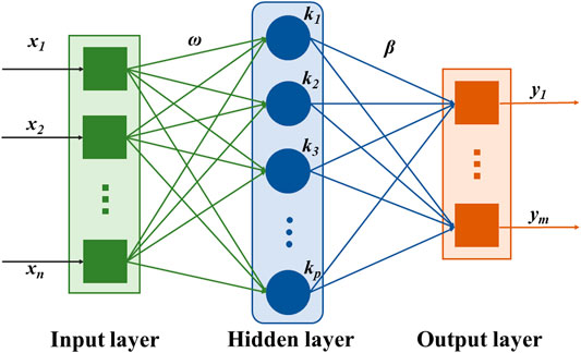
FIGURE 1. Structure of single hidden layer neural network.

For N input samples, x_i is the ith group of the input data, and it equals [x_i1, x_i2, … ,x_in]^T∈Rⁿ. The prediction result y is mathematically expressed as follows [24]:

${\mathit{y}}_i={\displaystyle \sum _{j=1}^p{\mathit{\beta }}_j{h}_j\left({\mathit{x}}_i\right)}={\displaystyle \sum _{j=1}^p{\mathit{\beta }}_j\sigma \left({\mathit{w}}_j\cdot {\mathit{x}}_i+b_j\right)}i=1,\dots ,N,(1)$

where p is the number of hidden nodes, β_j= [β_j1, β_j2, … ,β_jm]^T∈R^m is the weight vector that connects the jth hidden node and the output nodes, h_j(x) is the output function of the hidden nodes, w_j= [w_j1, w_j2, … ,w_jn]^T∈Rⁿ is the weight vector and connects the jth hidden node and the input nodes, b_j is the bias of the jth hidden node, and σ(x) is an excitation function. The predicted results can approximate the ideal outputs t_i with zero error as ∑||y_i – t_i|| = 0, if σ(x) is infinitely differentiable, where t_i is the corresponding label of x_i and it equals [t_i1,t_i2, … ,t_im]^T∈R^m. For simplicity, the above N equations can be rewritten as

$\mathbf{T}=\mathbf{Y}=\mathbf{H}\mathbf{{\rm B}},(2)$

where T = [t₁,t₂,...,t_N]^T is the ideal output, Y = [y₁,..., y_N]^T is the prediction result, H = [h (x₁),...,h (x_N)]^T is the hidden layer output matrix, and B = [β₁,β₂,...,β_p]^T is the output weight matrix. Thus, B can be obtained as follows [24]:

$\mathbf{{\rm B}}={\mathbf{H}}^{†}\mathbf{T}={\mathbf{H}}^T{\left(\mathbf{H}{\mathbf{H}}^T\right)}^{-1}\mathbf{T},(3)$

where H^† represents the generalized inverse matrix of H. To overcome the singular problems in calculating HH^T, the regularization coefficient I/e is added to the main diagonal in the diagonal matrix. Therefore, the output weight is rewritten as follows [24]:

$\mathbf{{\rm B}}={\mathbf{H}}^T{\left(\frac{\mathbf{I}}{e}+\mathbf{H}{\mathbf{H}}^T\right)}^{-1}\mathbf{T},(4)$

where I is the unit diagonal matrix and e is the punishment coefficient. The predicted result Y = HB can be obtained as

$\mathbf{Y}=h\left(\mathit{x}\right){\mathbf{H}}^T{\left(\frac{\mathbf{I}}{e}+\mathbf{H}{\mathbf{H}}^T\right)}^{-1}\mathbf{T}.(5)$

Here, we introduce the kernel function to enhance the stability of feature extraction. The kernel function is defined as follows [26]:

${\mathbf{\Omega }}_{\text{ELM}}=\mathbf{H}{\mathbf{H}}^T:{\mathbf{\Omega }}_{\text{ELM}i,j}=h\left({\mathit{x}}_i\right)\cdot h\left({\mathit{x}}_j\right)=K({\mathit{x}}_i,{\mathit{x}}_j).(6)$

For the linear indivisible low-dimensional data, the kernel function can map it into the high-dimensional space, yielding the data being divided. There are many kinds of kernel functions: the one used in this work is Gaussian function K (u, v) = exp (−γ||u–v||²), where γ = 1/(2σ²) and σ is standard deviation. Then, the output function of K-ELM classifier can be written as follows [26]:

$f\left(\mathit{x}\right)=\left[\begin{array}{l}K\left(\mathit{x},{\mathit{x}}_1\right)\\ ⋮\\ K\left(\mathit{x},{\mathit{x}}_N\right)\end{array}\right]{\left(\frac{\mathbf{I}}{e}+{\mathbf{\Omega }}_{\text{ELM}}\right)}^{-1}\mathbf{T}.(7)$

Due to the adoption of kernel function, the number of hidden neurons is self-adapted. Thus, the simple and effective K-ELM method has great potential in the field of underwater acoustic source localization.

Ocean Underwater Source Localization Using K-ELM

Physical Signal Model

Considering a single narrowband sound source impinges on a vertical linear array of M sensors formed with FOHP in a far-field scenario. The measured sound pressure field is initiated with a source of frequency ω at the range y and the depth z. Considering the presence of noise during the transport, the sound pressure field can be expressed in frequency domain as follows [4]:

$\mathbf{x}\left(\omega \right)=\left(1+\alpha \left(\omega \right)\right)\mathit{g}\left(\omega ,\mathit{\theta },\mathit{y},\mathit{z}\right)s\left(\omega \right)+\mathit{n}\left(\omega \right),(8)$

where x(ω) = [x₁(ω), x₂(ω), …, x_M(ω)]^T is the measured pressure field at frequency ω obtained by taking the discrete Fourier transform of the received pressure field for a period of observation times, α(ω) and n(ω) are the complex multiplicative noise and the additive noise, s(ω) is the source spectrum at frequency ω, and g (ω, θ, y, z) is the transfer function related to the frequency ω, environment parameter θ, source range y, and depth z. Furthermore, the pressure field of far-field broadband source with frequency ω_q∈[ω₁, ω_Q] at position (y, z) can be written as follows [6]:

$\mathbf{x}=\mathit{G}\left(\mathit{\theta },\mathit{y},\mathit{z}\right)\tilde{\mathbf{s}}+\mathbf{n},(9)$

where Q is the number of discrete frequency bins, x = [x^T (ω₁), …, x^T (ω_Q)]^T is defined as an extended vector for both narrowband and broadband cases, n = [n^T (ω₁), …, n^T (ω_Q)]^T is defined similarly with x, $\tilde{\mathbf{s}}$= [(1+ α(ω₁))s (ω₁), …, (1+α(ω_Q))s (ω_Q)]^T is a Q-dimensional vector, and G (θ, y, z) is a $QM\times Q$ matrix written as follows [23]:

$\mathit{G}\left(\mathit{\theta },\mathit{y},\mathit{z}\right)=\left[\begin{array}{cccc}\mathit{g}\left({\omega }_1,\mathit{\theta },\mathit{y},\mathit{z}\right)& 0& \dots & 0\\ 0& g\left({\omega }_2,\mathit{\theta },\mathit{y},\mathit{z}\right)& \dots & 0\\ ⋮& ⋮& \ddots & ⋮\\ 0& 0& \dots & g\left({\omega }_Q,\mathit{\theta },\mathit{y},\mathit{z}\right)\end{array}\right].(10)$

The multiplicative noise is modeled as a complex random perturbation factor α = |α|exp (jϕ), which is commonly assumed to be a complex Gaussian distribution. The perturbation factor level is defined as 10 log₁₀|α(ω)|² (dB). The additive noise is modeled as a complex Gaussian distribution with mean value 0 and variance δ². Due to the decrease of the signal level with range increment, the signal-to-noise ratio (SNR) is defined at the most distant range bin as follows [18]:

$\text{SNR}=10{\log }_{10}\frac{{\displaystyle \sum _{i=1}^M{\left|x_i\left(\omega \right)\right|}^2/M}}{{\delta }^2}\left(\text{dB}\right).(11)$

K-ELM Method for Source Localization

Here, K-ELM is employed for source localization, which is achieved as follows:

1) Simulate the acoustic pressure signal with respect to different ranges and depths.

2) Add noise with different SNRs onto the ideal simulation signals to generate the noised signal for testing.

3) Preprocess the input data. The discrete Fourier transform is conducted to transform the measured sound pressure signal into the frequency domain. Then, the SCMs are calculated and vectorized to be the input data of the K-ELM model.

4) Utilize the SCMs of ideal signals as the training data, and adopt the SCMs of noised signals as the testing data.

5) Train two K-ELM models for range and depth prediction on the training set.

6) Predict the source range and the depth on testing set using the well-trained K-ELM models.

The training samples are simulated under different ranges and depths. The range of acoustic source is changed from 1 km to 8 km with a step of 5 m, and the depth of acoustic source varies from 10 m to 200 m with a step of 1 m. Therefore, the number of training samples is 1,400 and 190 for range and depth localization training set, respectively. The testing samples are acquired by adding noise to training samples, among which, 561 samples are selected to build the test set.

The structure of K-ELM is self-adaptive. Thus, the input neurons and hidden neurons do not need to be designed. The only parameter to be trained is the output weight matrix. We apply the K-ELM to source localization in both narrowband case (Q = 1, single frequency) and broadband case (Q ≥ 2, multiple frequencies). Note that the signals with different bandwidth are divided into several groups, and the training and evaluation are conducted utilizing data within the same groups.

Before utilizing the K-ELM for source localization, data preprocessing is conducted to extract the feature and reduce the data redundancy. Firstly, to reduce the effect of the source spectrum s(ω), the complex sound pressure p(ω) at the frequency ω is normalized by the following [23].

$\tilde{\mathit{x}}\left(\omega \right)=\frac{\mathit{x}\left(\omega \right)}{\Vert \mathit{x}\left(\omega \right)\Vert }=\frac{\mathit{x}\left(\omega \right)}{\sqrt{{\mathit{x}}^H\left(\omega \right)\mathit{x}\left(\omega \right)}}=\frac{\mathit{x}\left(\omega \right)}{\sqrt{{\displaystyle \sum _{i=1}^M{\left|\mathit{x}\left(\omega \right)\right|}^2}}},(12)$

where ||·|| denotes the norm and (·)^H denotes the complex conjugate transpose. In order to obtain an accurate localization result, the normalized SCM, C(ω), is usually formed from the normalized sound pressure p_s(ω) at the sth snapshot and averaged over N_s snapshots.

$C\left(\omega \right)=\frac{1}{N_s}{\displaystyle \sum _{s=1}^{N_s}\tilde{x}\left(\omega \right){\tilde{x}}_s^H\left(\omega \right)},(13)$

where Ns is the number of snapshots and C(ω) is a conjugate symmetric matrix. Thus, only the upper triangular matrix entries are enough. The real and imaginary parts of these entries are separated and vectorized to a 1D vector $\overline{C}\left(\omega \right)$, which consists of M × (M +1) elements in single frequency case (Q = 1). For the broadband case (Q ≥ 2), the input data is constructed by $\overline{C}\left(\omega \right)$with different single frequencies as [${\overline{C}}^T\left({\omega }_1\right)$, ${\overline{C}}^T\left({\omega }_2\right)$, …, ${\overline{C}}^T\left({\omega }_Q\right)$]^T. Each $\overline{C}\left({\omega }_q\right)$ is the same with the single frequency case.

With the 5 m and 1 m interval, 1,500 groups and 190 groups of training data with respect to range and depth are simulated. The normalized SCM at each range is formed over two 1-s snapshots, according to Eq. (13). In this work, the number of elements of VLA is 21. Thus, the number of input vectors is 21 × (21 + 1)=462 for narrowband case and $21\times \left(21+1\right)\times Q=462Q$for broadband case.

Results and Discussion

Simulations are conducted to evaluate the performance of the proposed methods. In this section, we use KRAKEN [27] to simulate the acoustic data in a shallow water waveguide which is similar to that of the SWellEx-96 experiment [28] as illustrated in Figure 2. The environment parameters are considered as range-independent and depth-independent. Here, four layers are considered, that is, water layer, sediment layer, mudstone layer, and seafloor half-space. The SSP of water layer is shown in Figure 2. The parameters of the environment are given in Table 1.

FIGURE 2

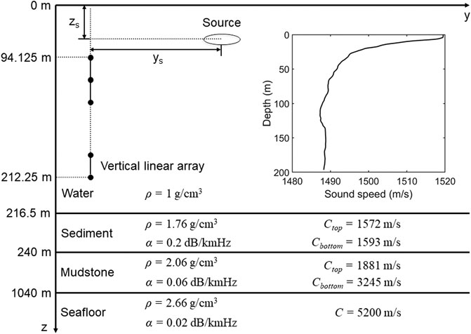
FIGURE 2. Schematic diagram of the simulated acoustic environmental model.

TABLE 1

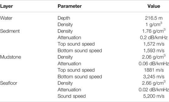
Table 1. Parameters of the environment.

Then, the source range varies from 1 km to 8 km with a step of 5 m, and the depth is changed from 10 m to 200 m with a step of 1 m. The source signal is assumed to contain a series of multi-tones ({49, 94, 148, 235, 399} Hz) which is the same as SWellEx-96 experiment. The VLA consisted of 21 hydrophones spanning a depth of 94.125 m–212.25 m with uniform inter-sensor space as in the SWellEx-96 experiment. The sampling rate is set as 1,500 Hz.

We adopt two measures to quantify the performance of K-ELM in source localization task. There are MAPE and 10% error interval. These two measures are defined as

$MAPE=\frac{100}{L}{\displaystyle \sum _{i=1}^L\left|\frac{R_{gi}-R_{ti}}{R_{ti}}\right|},(14)$

$R_u,R_l=R_t\times \left(1\pm 10\%\right),(15)$

where L is the sample number in the test set. R_g and R_t are the predicted range by K-ELM and the true range, respectively. The 10% error interval defines the upper bound R_u and lower bound R_l with respect to the truth range R_t.

The K-ELM model is evaluated under three SNRs: 5 dB, 0 dB, and −5 dB. For each SNR, both narrowband and broadband sources are considered. The perturbation factor level is set to −10 dB for all cases.

Figure 3 shows the localization results of K-ELM under different SNRs in narrowband and broadband cases. For simplicity, only the results of 235 Hz and {94, 148, 388} Hz are presented in Figure 3. The predicted ranges are plotted as the red circle, the true ranges are plotted as the blue line, and the 10% error interval is also plotted as the gray shadow area. As shown in Figure 4, the range localization accuracy degrades with the decrease of the SNR. For narrowband case, the prediction results are similar at 5 dB and 0 dB and show great decline at −5 dB, especially on the ranges near both ends. But most predicted ranges are still within the 10% error interval. The MAPE of this case is 8.27. For broadband case, the performance is better than that of narrowband case, especially at low SNR of −5 dB with MAPE of 0.11. With the decrease of SNR, the prediction results show slight fluctuation and degradation. The MAPE of K-ELM with {94 148 388} Hz signal is 0.11, which is 8-fold less than narrowband case. The MAPE of MFP method with {94 148 388} Hz signal condition is 33.5%, which is greatly larger than K-ELM.

FIGURE 3

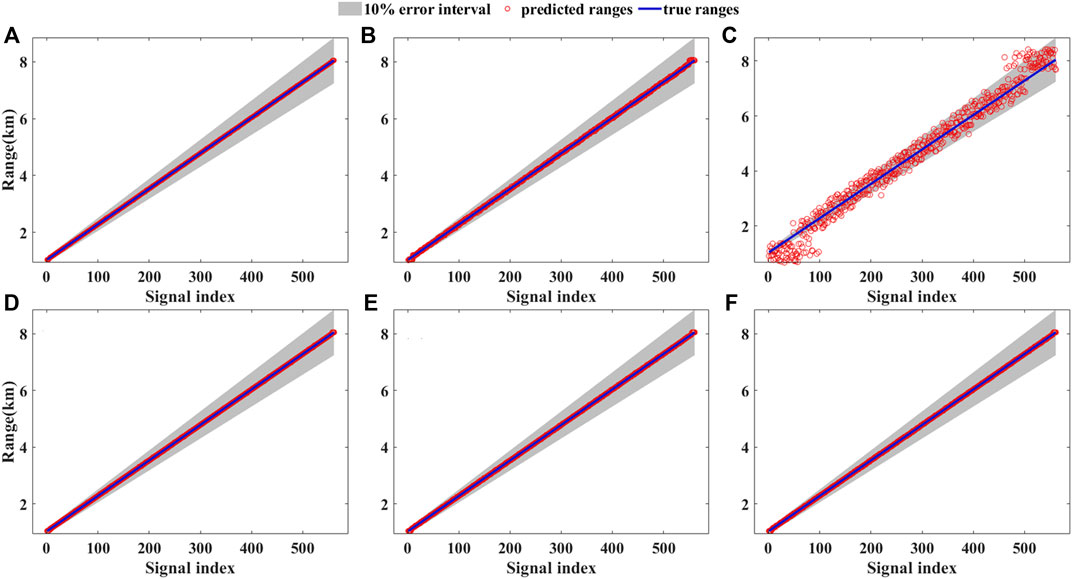
FIGURE 3. Range localization results with various SNRs by K-ELM. (Top) The narrowband case of 235 Hz. (Bottom) The broadband case of {94,148 388} Hz with SNR of (A) (D) 5 dB, (B) (E) 0 dB, and (C) (F) -5 dB.

FIGURE 4

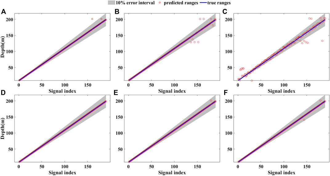
FIGURE 4. Depth localization results with various SNRs by K-ELM. (Top) The narrowband case of 148 Hz. (Bottom) The broadband case of {49 94,235} Hz with SNR of (A) (D) 5 dB, (B) (E) 0 dB, and (C) (F) -5 dB.

Next, more detailed MAPEs with different frequencies and SNRs are given in Table 2. It can be seen that the performance of K-ELM under broadband case is much better than narrowband case. For example, the broadband signal consisting of two narrowband signals with low frequencies, {49 94} Hz, achieves better performance than that of 49 Hz and 94 Hz cases, even than the best performance in narrowband case achieved by 388 Hz. In particular, the accuracy of broadband case is much better than narrowband case at low SNRs (<0 dB), where the minimum MAPEs for narrowband and broadband case are 5.05 and 0.07, respectively. The minimum MAPE at low SNR is reduced by 72 times. On the other hand, some inner rules exist in narrowband and broadband cases. For narrowband case, the accuracy increases with the increment of signal frequency, while for broadband case, the accuracy is influenced by two factors, that is, the number of frequency bins and the highest frequency of broadband signal. With the increase in the number of frequency bins, the MAPE decreases gradually. Meanwhile, for the broadband signal which has the same frequency bins, the signal with higher frequency achieves better accuracy; for example, MAPEs of {94 148 388} Hz case and {49 94 235} Hz case at −5 dB are 0.11 and 0.16, respectively. To draw a conclusion, multiple-frequency source signals and high frequency signals contain more information, leading to better performance. At last, the time for processing 560 signals with K-ELM model is about 0.05 s. That is to say, the proceeding speed is fast, which is desirable for real-time testing in practice.

TABLE 2

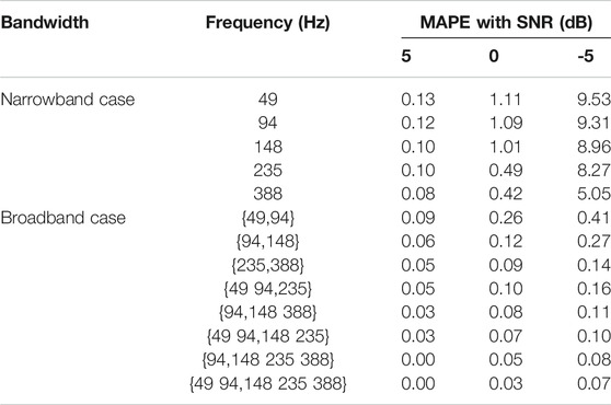
Table 2. Range prediction results with narrowband and broadband cases.

The performance of source depth localization by K-ELM method is further tested. The depth prediction is regarded as classification task as well. The source depth is simulated from 10 m to 200 m with a step of 1 m. The prediction results with three SNRs under narrowband and broadband case are illustrated in Figure 4. For simplicity, the results of 235 Hz and {94 148 388} Hz, which are different from those in range prediction, are presented in Figure 4.

According to Figure 4, the performance of localization shows similar rule to that in broadband case. The accuracy degrades with the decrease of SNR in both narrowband and broadband case. The adoption of broadband signal greatly improves the performance greatly as well. At low SNR (−5 dB), the MAPE of narrowband case is 7.53%, and that of broadband case is 0.09%, which is reduced 87 times. At the same condition, the MAPE of MFP under broadband case is 28.7%. The detailed MAPEs of depth prediction under different frequencies and SNRs are given in Table 3 similar to the range localization. The MAPE distribution of Table 3 shows similar rule to Table 2. The MAPEs of depth prediction are relatively smaller than range prediction. The minimum MAPEs at low SNR for narrowband and broadband are 4.82 and 0.04, respectively. It is reduced by 80 times.

TABLE 3

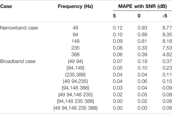
Table 3. Depth prediction results with narrowband and broadband cases.

The K-ELM algorithm shows reasonable predictions on acoustic source localization, which demonstrate its advantages on signal processing and always provide a global optimum without the need of iterative tuning.

Conclusion

In summary, a machine learning method, K-LEM, is proposed to achieve the single ocean underwater acoustic source localization. Sound pressure signals received from fiber-optic hydrophone with different frequencies and SNRs are utilized to investigate the performance of K-ELM for source localization. The acoustic pressure signal measured by VLA is transformed to frequency domain and preprocessed into normalized SCM as the input of the K-ELM. These SCMs are classified into different ranges or depths by K-ELM algorithm. The results show that K-ELM performs well in both range and depth localization task under various frequencies and SNRs. In particular, in case of SNR with −5 dB, the least MAPEs of range localization for narrowband and broadband cases are 0.08 and 0, and those of depth localization for narrowband and broadband case are 0.06 and 0.00, respectively. Meanwhile, composition of narrowband signals can greatly improve the prediction accuracy. The maximum reductions of MAPE for range and depth localization are 136 and 146 times. Moreover, the processing time of K-ELM method for 560-group data is only 0.05 s, indicating the high processing speed in underwater acoustic source localization, which makes it possible for real-time testing. Thus, the K-ELM gives an accurate and effective way for ocean underwater source localization.

Data Availability Statement

The raw data supporting the conclusions of this article will be made available by the authors, without undue reservation.

Author Contributions

ZH and JH conceived and performed the papers collection and manuscript writing; PX and MN were involved in the paper writing; KL and GL were involved in the paper review and editing. All the authors contributed to the discussion on the results for this manuscript.

Conflict of Interest

The authors declare that the research was conducted in the absence of any commercial or financial relationships that could be construed as a potential conflict of interest.

References

1. Wu Y, Li G, Hu Z, Hu Y. Unambiguous directions of arrival estimation of coherent sources using acoustic vector sensor linear arrays. IET Radar, Sonar Navig (2015) 9:318–23. doi:10.1049/iet-rsn.2014.0191

CrossRef Full Text | Google Scholar

2. Cao C, Hu Z, Xiong S, Hu Y. Transmission-link-induced intensity and phase noise in a 400-km interrogated fiber-optics hydrophone system using a phase-generated carrier scheme. Opt Eng (2013) 52:096101. doi:10.1117/1.Oe.52.9.096101

CrossRef Full Text | Google Scholar

3. Bogart CW, Yang TC. Comparative performance of matched‐mode and matched‐field localization in a range‐dependent environment. J Acoust Soc Am (1992) 92:2051–68. doi:10.1121/1.405257

CrossRef Full Text | Google Scholar

4. Baggeroer AB, Kuperman WA, Mikhalevsky PN. An overview of matched field methods in ocean acoustics. IEEE J Oceanic Eng (1993) 18:401–24. doi:10.1109/48.262292

CrossRef Full Text | Google Scholar

5. Mirkin AN. Maximum likelihood estimation of the locations of multiple sources in an acoustic waveguide. J Acoust Soc Am (1993) 93:1205. doi:10.1121/1.405522

CrossRef Full Text | Google Scholar

6. Soares C, Jesus SM. Broadband matched-field processing: coherent and incoherent approaches. J Acoust Soc Am (2003) 113:2587–98. doi:10.1121/1.1564016

PubMed Abstract | CrossRef Full Text | Google Scholar

7. Mantzel W, Romberg J, Sabra K. Compressive matched-field processing. J Acoust Soc Am (2012) 132:90. doi:10.1121/1.4728224

PubMed Abstract | CrossRef Full Text | Google Scholar

8. Mantzel W, Romberg J, Sabra KG. Round-robin multiple-source localization. J Acoust Soc Am (2014) 135:134–47. doi:10.1121/1.4835795

PubMed Abstract | CrossRef Full Text | Google Scholar

9. Yang TC. Data-based matched-mode source localization for a moving source. J Acoust Soc Am (2014) 135:1218–30. doi:10.1121/1.4863270

PubMed Abstract | CrossRef Full Text | Google Scholar

10. Verlinden CM, Sarkar J, Hodgkiss WS, Kuperman WA, Sabra KG. Passive acoustic source localization using sources of opportunity. J Acoust Soc Am (2015) 138:EL54–9. doi:10.1121/1.4922763

PubMed Abstract | CrossRef Full Text | Google Scholar

11. Sazontov AG, Malekhanov AI. Matched field signal processing in underwater sound channels (Review). Acoust Phys (2015) 61:213–30. doi:10.1134/S1063771015020128

CrossRef Full Text | Google Scholar

12. Vasan R, Rowan MP, Lee CT, Johnson GR, Rangamani P, Holst M. Applications and challenges of machine learning to enable realistic cellular simulations. Front Phys (2020) 7:7. doi:10.3389/fphy.2019.00247

CrossRef Full Text | Google Scholar

13. Biamonte J, Kardashin A, Uvarov A. Quantum machine learning tensor network states. Front Phys (2020) 8:586374. doi:10.3389/fphy.2020.586374

CrossRef Full Text | Google Scholar

14. Zhang Y, Yu L, Zhengliang H, Cheng L, Sui H, Zhu H, et al. Ultrafast and accurate temperature extraction via kernel extreme learning machine for BOTDA sensors. J Lightwave Technol (2020) 39:1537–1543. doi:10.1109/JLT.2020.3035810

CrossRef Full Text | Google Scholar

15. Zhu H, Yu L, Zhang Y, Cheng L, Zhu Z, Song J, et al. Optimized support vector machine assisted BOTDA for temperature extraction with accuracy enhancement. IEEE Photon J. (2020) 12:1–14. doi:10.1109/JPHOT.2019.2957410

CrossRef Full Text | Google Scholar

16. Yu L, Cheng L, Zhang JL, Zhu HN, Gao XR. “Accuracy improvement for fine-grained image classification with semi-supervised learning,” in: Asia comm and photon conf.. Chengdu, IL: IEEE (2019). 1–3.

Google Scholar

17. Devlin J, Chang M, Lee K, Toutanova K. BERT: pre-training of deep bidirectional transformers for language understanding. Preprint repository name [Preprint] (2018) Available from: arXiv: 1810.04805 (Accessed October 11, 2018).

18. Dabiri Y, Van der Velden A, Sack KL, Choy JS, Kassab GS, Guccione JM. Prediction of left ventricular mechanics using machine learning. Front Phys (2019) 7:117. doi:10.3389/fphy.2019.00117

PubMed Abstract | CrossRef Full Text | Google Scholar

19. Niu H, Gerstoft P. Source localization in underwater waveguides using machine learning. J Acoust Soc Am (2016) 140:3232. doi:10.1121/1.4970220

CrossRef Full Text | Google Scholar

20. Niu H, Reeves E, Gerstoft P. Source localization in an ocean waveguide using supervised machine learning. J Acoust Soc Am (2017) 142:1176–88. doi:10.1121/1.5000165

PubMed Abstract | CrossRef Full Text | Google Scholar

21. Niu H, Ozanich E, Gerstoft P. Ship localization in Santa Barbara Channel using machine learning classifiers. J Acoust Soc Am (2017) 142:EL455–EL460. doi:10.1121/1.5010064

PubMed Abstract | CrossRef Full Text | Google Scholar

22. Huang Z, Xu J, Gong Z, Wang H, Yan Y. Source localization using deep neural networks in a shallow water environment. J Acoust Soc Am (2018) 143:2922–32. doi:10.1121/1.5036725

PubMed Abstract | CrossRef Full Text | Google Scholar

23. Wang Y, Peng H. Underwater acoustic source localization using generalized regression neural network. J Acoust Soc Am (2018) 143:2321–31. doi:10.1121/1.5032311

PubMed Abstract | CrossRef Full Text | Google Scholar

24. Huang G-B, Zhu Q-Y, Siew C-K. Extreme learning machine: theory and applications. Neurocomputing (2006) 70:489–501. doi:10.1016/j.neucom.2005.12.126

CrossRef Full Text | Google Scholar

25. Huang G, Huang GB, Song S, You K. Trends in extreme learning machines: a review. Neural Netw (2015) 61:32–48. doi:10.1016/j.neunet.2014.10.001

PubMed Abstract | CrossRef Full Text | Google Scholar

26. Huang GB, Zhou H, Ding X, Zhang R, Cybernetics PB. Extreme learning machine for regression and multiclass classification. IEEE Trans Syst Man Cybern B Cybern (2011) 42:513–29. doi:10.1109/TSMCB.2011.2168604

PubMed Abstract | CrossRef Full Text | Google Scholar

27. Porter MB. The KRAKEN normal mode program. Washington DC: Naval Research Lab (1992).

28. Murray J, Ensberg D. The SWellEx-96 experiment. Available at: http://swellex96.ucsd.edu/ (Accessed April 29, 2003).