 Nora Höfner1
 Peter Hömmen
 Antonino Mario Cassarà
 Rainer Körber
94% of researchers rate our articles as excellent or good
Learn more about the work of our research integrity team to safeguard the quality of each article we publish.
Find out more
ORIGINAL RESEARCH article
Front. Phys., 26 April 2021
Sec. Medical Physics and Imaging
Volume 9 - 2021 | https://doi.org/10.3389/fphy.2021.647376
This article is part of the Research TopicInnovations in MR Hardware from Ultra-Low to Ultra-High FieldView all 14 articles
The possibility to directly and non-invasively localize neuronal activities in the human brain, as for instance by performing neuronal current imaging (NCI) via magnetic resonance imaging (MRI), would be a breakthrough in neuroscience. In order to assess the feasibility of 3-dimensional (3D) NCI, comprehensive computational and physical phantom experiments using low-noise ultra-low-field (ULF) MRI technology were performed using two different source models within spherical phantoms. The source models, consisting of a single dipole and an extended dipole grid, were calibrated enabling the quantitative emulation of a long-lasting neuronal activity by the application of known current waveforms. The dcNCI experiments were also simulated by solving the Bloch equations using the calculated internal magnetic field distributions of the phantoms and idealized MRI fields. The simulations were then validated by physical phantom experiments using a moderate polarization field of 17 mT. A focal activity with an equivalent current dipole of about 150 nAm and a physiologically relevant depth of 35 mm could be resolved with an isotropic voxel size of 25 mm. The simulation tool enabled the optimization of the imaging parameters for sustained neuronal activities in order to predict maximum sensitivity.
The realization of ultra-low-field (ULF) magnetic resonance imaging (MRI), i.e., MRI in the μT-regime, was possible when new, very sensitive superconducting quantum interference devices (SQUID) sensors could be used to detect nuclear spin precession [1, 2], and, within a few years, several ULF scanners have been developed [3–7]. As the magnetization of the examined volume scales with the surrounding magnetic field, ULF MRI has to cope with a lower signal-to-noise ratio (SNR) compared to high-field MRI—typically employing fields on the order of 1 T and above. Despite different measures to mitigate this low SNR, e.g., pre-polarization, only comparably large voxel sizes in the mm-range could be reached until now in in vivo applications. However, the possibility of using ULF MRI for functional imaging is promising motivating the development effort albeit with some compromises regarding spatial resolution. Consequently, imaging of neuronal magnetic fields via their interaction with the spin population, coined neuronal current imaging (NCI), was soon investigated by attempting to directly detect the influence of biomagnetic signals on the phase and relaxation of the nuclear spin precession in the ultra-low-field regime [8].
The successful implementation of NCI would be of particular significance, as currently available non-invasive methods for imaging brain function, such as functional MRI (fMRI), magnetoencephalography (MEG), or electroencephalography (EEG) suffer from either poor temporal resolution or error-prone spatial localization accuracy [9]. The possibility of NCI via high-field MRI was studied intensively applying different approaches [10–12]. Unfortunately, the results were either inconclusive due to a lack of sensitivity of the MRI signal to evoked neuronal activity [13] or irreproducible because of the dominating blood oxygen level-dependent (BOLD) effect [14]. In contrast, owing to the low magnetic field, ULF MRI has the advantage that the BOLD effect becomes negligible [15].
Several phantom studies have explored possible implementations of NCI using ULF MRI, and have highlighted the necessary technical and methodical improvements [16–19]. These studies suggest two different approaches. The so-called AC or resonant mechanism proposes the use of the magnetic field generated by the neuronal currents itself to manipulate the spin dynamics. This condition would be best met by tuning the Larmor frequency to match the main frequencies of the neuronal activity (resonant condition) [16–18, 20] and the MR signal would be produced exclusively by the proton spins in close proximity to the source. The second approach, called the DC mechanism, aims at measuring the minuscule phase perturbation generated by the very weak neuronal magnetic field [16–18]. One possible implementation is based on the acquisition of MR images in the presence and absence of evoked activity. A difference image would then reveal the effect of the neuronal magnetic field. The effectiveness of the two approaches has been demonstrated in multiple phantom studies; however, a fundamental lack of sensitivity has to be overcome for in vivo applications. Körber et al. [18] showed that for sufficiently long-lasting neuronal activities, the DC mechanism could feature larger contrast-to-noise ratio (CNR) than the AC mechanism. As different simulation studies on NCI using high-field MRI showed, the specific spatial and temporal characteristics of the neuronal currents affect the measurable phase and relaxation changes [20–25].
Motivated by this, and expanding on our earlier phantom experiments [17, 18, 26], we developed a computational framework that can be used to simulate 3-dimensional (3D) dcNCI sequences based on ULF MRI. It is centered on our low-noise ULF-MRI hardware and on a well-characterized long-lasting, monophasic neuronal activity which can be evoked by median nerve stimulation. We strove for current dipole phantoms, which could be manufactured with a well-defined geometry facilitating the simulation of their internal and external fields. Measuring their far-field distribution using a multi-channel SQUID system allowed the determination of their equivalent current dipole (ECD) strength for a given applied current. The simulated internal field distributions served as input to an analytic MR solver to characterize the dcNCI signature of the phantoms for multiple configurations and to optimize the imaging sequence for the existing experimental 3D ULF-MRI setup. The validated framework was then used to assess the feasibility and requirements toward in vivo dcNCI.
The experimental phantom study was performed using low-noise ULF-MRI hardware [27] at the Physikalisch-Technische Bundesanstalt (PTB), Berlin, as shown in Figure 1A. The system deploys resistive room temperature MRI coils and is located inside a moderately magnetically shielded room (MSR) which features a residual field of <1.5 nT after degaussing [28].
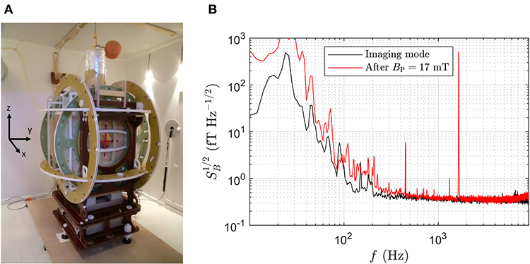
Figure 1. (A) ULF-MRI setup inside magnetically shielded room. (B) Field noise (referred to the bottom pick-up loop) of the 3D ULF-MRI setup in imaging mode and after a polarizing pulse of BP=17 mT. The signal at 1,645 Hz was obtained with B0=38.6 μT and dBx/dx=2.4 μT/m. Data were captured 25 ms after initiating BP turn-off (compare to validation measurement shown in Figure 4).
Helmholtz coils generate the homogeneous detection field B0 along x and the π/2-pulse (Bπ/2) along the y-direction, while a Maxwell coil provides the frequency encoding gradient GF = dBx/dx and two orthogonal biplanar gradient coils generate the phase encoding gradients GPh = dBx/dy and dBx/dz. A self-shielded coil provides the homogeneous polarizing field BP along x while simultaneously reducing transient effects from the MSR. The coils, with the parameters given in Table 1, are powered by low-noise current sources placed outside the MSR that are disconnected during data acquisition, if possible.
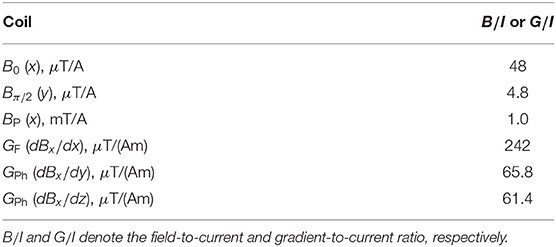
Table 1. Coil parameters of the PTB ULF-MRI system.
For signal detection we use our single-channel ultra-low-noise SQUID system that is operated inside the low intrinsic noise dewar LINOD2 [29]. A SQUID current sensor is inductively coupled to a superconducting pick-up coil designed as an axial second-order gradiometer with an overall baseline of 125 mm and a diameter of 45 mm. Since a longitudinal gradient is applied for frequency encoding, this configuration and a very low-noise current source with 470 pA Hz−1/2 driving the GF coil (active during data acquisition) are necessary to reduce noise contributions to a negligible level. A transverse gradient can be used to relax these requirements. The gradiometer dimensions also maximize the SNR with respect to the sustained neuronal source, which was estimated to have a distance of about 50 mm (source-scalp distance 35 mm, see below) to the lower pick-up coil of the gradiometer [30]. When the single-channel SQUID system is operated within the 3D ULF-MRI setup in imaging mode, i.e., with B0 and GF coils powered, the total field noise (referred to the bottom pick-up loop) is about 380 aT Hz−1/2 for frequencies above 1 kHz and does not increase after application of the polarizing pulse (see Figure 1B).
Current dipole phantoms mimic the underlying focal neuronal activity, which is a sustained, monophasic response following electrostimulation of the median nerve. Its characterization was carried out in previous MEG studies, as shown in Figure 2A [18]. The activity is located at a depth of about 35 mm to the scalp surface within the somatosensory cortex SII with a maximum ECDmax of about 50 nAm. A time-stable dipolar field indicates a focal activity which decays over about 1 s after stimulation. The derived waveform of variable length, depending on the dcNCI parameters, starts after the last stimulus which excludes artifacts in a potential in vivo experiment.
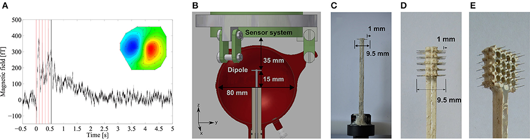
Figure 2. (A) MEG field trace of sustained activity after five electrostimuli of the median nerve (red lines) and the field map averaged from 0.5 to 1.0 s (inset), adapted with permission from Körber et al. [18]. The waveform of variable length (dependent on dcNCI parameters) starts at 0.55 s, as indicated by the black line. (B) Head phantom positioned below the dewar with the integrated single current dipole within a conducting solution. (C) Single current dipole. (D) 5 × 5 dipole grid simulating an extended source. (E) Extended source phantom showing the array of holes facilitating the flow of return currents to avoid cross currents.
In Figure 2B, the phantom positioned below the ULF-MRI SQUID system is shown with the dipole at a depth of 35 mm corresponding to the depth of the physiological model. The NCI phantom with an 80 mm diameter is filled with a CuSO4 and NaCl solution featuring the conductivity σSol=0.325 S/m and the ULF-MR parameters of brain tissue with T1 = T2=100 ms [31]. A gap of 10 mm between the phantom and the dewar simulates the skull which has a negligible MR signal.
The scalable current dipole concept is based on commercially available printed-circuit-boards (PCBs), allowing a precise fabrication of various arrangements and numbers of current dipoles. The electrodes are made from insulated Pt wire (diameter 125 μm) with a total length of 9.5 mm. At both wire-ends 1 mm of the insulation is removed. Two phantoms were fabricated: a single current dipole consisting of two electrodes pointing apart, as shown in Figure 2C, and a dipole grid with 5 × 5 current dipoles arranged in a square lattice with a dipole spacing of 2 mm, as shown in Figures 2D,E. If the grid dipoles were mounted on a solid, continuous plate, a slightly higher current would flow in the outside electrodes, since the shorter return path through the conducting medium leads to a lower resistance. Therefore, the mounting plate of the grid was assembled with holes to minimize this effect. Simulations described below also confirmed that this suppresses cross currents between electrodes on each side of the grid. The minute additional potential drop from the base to the tip of the electrode due to the current is practically identical for all individual electrodes.
Currents of up to 80 μA were applied using a home-built, battery-powered, voltage-controlled current source enabling a faithful reproduction of arbitrary waveforms. The phantoms were calibrated by measuring the external magnetic field map for a known drive current with 97 sensors of the 304-channel SQUID system of PTB [32]. Those were close to the phantom and more distant sensors were not used, since they would contain mostly noise and hence negligible signal information. Performing an equivalent current dipole reconstruction allowed the determination of the effective dipole length.
The 3D ULF-MRI sequence was a gradient echo sequence and is displayed in Figure 3. The polarizing field BP of 17 mT, applied for 500 ms (tP) including a 150 ms ramp, is turned off adiabatically over 15 ms (tOff) until it is aligned with the permanent detection field B0 of 38.6 μT. A π/2-pulse of length 2.43 ms (tRF) initiates the precession of the magnetization M. Then, one frequency encoding gradient GF (dBx/dx) and two phase encoding gradients GPh (dBx/dy), GPh (dBx/dz) are applied for the spatial encoding of the three dimensions (k-space filling). For anatomical imaging, tPh should be as short as possible to minimize signal loss due to relaxation. A tPh of 30 ms was used, as in our previous in vivo imaging [27]. Detecting up to four consecutive echoes leads to an overall measurement time of about 800 ms, including the polarization period. A pause of 2 s between the individual measurements avoids overheating of the uncooled polarizing coil. Table 2 summarizes the imaging parameters.
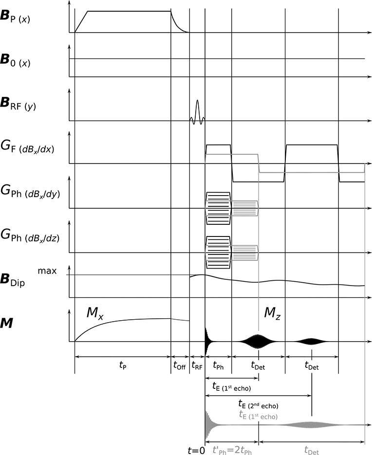
Figure 3. Schematic 3D ULF-MRI sequence. After adiabatic turn-off of BP and a subsequent π/2-pulse, phase encoding gradients GPh and a frequency encoding gradient GF are utilized and echoes are generated by reversing GF. The dipole field BDip is applied permanently during the entire encoding period. Exemplary echoes are shown for phase times tPh and (gray color). In the latter, the gradient strengths are halved giving the same k-space coverage. Time periods t are differently scaled.
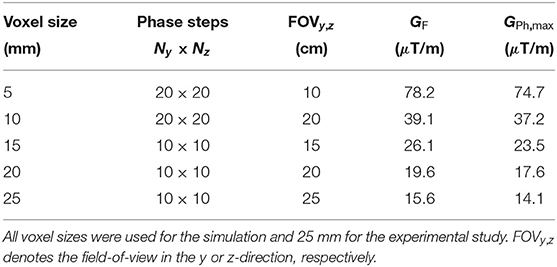
Table 2. Imaging parameters for a phase time tPh=30 ms and sampling frequency of 20 kHz resulting in isotropic voxel sizes.
In order to guarantee maximum phase accumulation, and therefore the largest detectable signal, the dipoles are oriented perpendicularly to B0. In this way, BDip are parallel and anti-parallel to B0 just above and below the dipole, respectively. The applied dipole field, as shown in Figure 3, was derived from the measured temporal amplitude profile of a somatosensory evoked long-lasting activity. BDip affects the precession during the spatial encoding and the readout of the echo signal causing phase and frequency shifts. The expectedly small frequency changes in the millihertz range [33] are visualized using a difference image technique. During one measurement the dipole field BDip is active (on). A second measurement serves as a reference in which the dipole is not driven and BDip=0 (off). Subtracting the two data sets (on−off) in the time domain reveals the affected 1H-spins in the difference image. An additional reference measurement (off′) allows screening for artifacts by calculating a difference image (off−off′) which should not show a residual above the noise level.
The measurement of the very small BDip of several hundred pT imposes high demands on the 3D ULF-MRI setup, requiring a high SNR, as well as a high stability of the applied magnetic fields. In order to reduce the influence of magnetic field drifts due to current drifts in the detection field coil or changes of the background field within the magnetically shielded room, we alternate the order of the measurements with and without the applied dipole field. Nevertheless, low-frequency drifts mainly from the current source driving the detection coil lead to measured equivalent frequency shifts of up to ±27 mHz for successive measurements. This causes artifacts in the difference image, masking the influence of the dipole field. To correct for these, the current through the detection coil was simultaneously measured by acquiring the voltage across a precise sense resistor, RS=1Ω, for subsequent phase correction. At a Larmor frequency of 1,645 Hz the maximum frequency shifts correspond to ~16 ppm (parts per million), which translate to a current change of 13 μA in the detection coil or 13 μV over the sense resistor. After a ground isolation stage, this voltage is acquired with a 24-bit digitizer. The noise of 65 nV Hz−1/2 is dominated by the isolation stage and would result in 5.8 μVrms given the 8 kHz measurement bandwidth. Therefore, digital low-pass filtering with fc=50 Hz is applied to allow sub-μV resolution.
The number of measurements per setting, i.e., dipole on or dipole off, was 400 so that for voxel sizes of 15, 20, and 25 mm averaging could be implemented to increase sensitivity. The overall measurement time amounted to ~40 min (on and off) and to ~60 min if the additional reference off′ was taken, respectively.
The magnetic flux changes during the data acquisition tDet result from the induced echo signal Mz(t) (see Figure 3), as well as interfering field changes of various sources. Starting the data analysis, we apply first a fitting routine and subtract low-frequency transients. These result from transient responses of the shielded room, background field changes or small vibrational movements of the sensor system within the gradient field. A truncation to remove filter artifacts leads to a ~10% larger voxel size in the x-direction.
The Hilbert-Transformation is applied to the real-valued measured data to derive the analytical signal sa(tn), with tn denoting a discrete step of time t. This is then demodulated using two synthetic waveforms c1 and c2(tn) according to:
where c1 adjusts the initial phase, accumulated during the phase encoding period tPh, and, c2(tn) takes time varying phase changes during data acquisition into account, and, fL is the Larmor frequency. A further phase correction is applied, in order to adjust the boundary between two slices to the position of the current dipole in the phantom, thus avoiding signal loss due to signal cancellation within one voxel reducing the difference signal amplitude.
Subsequently, performing the 3D Fourier transform of the time-domain difference signal Δs = son−soff and calculating its amplitude image ΔS, the highest possible CNR and reduced influence of the detection field instabilities can be achieved. For further analysis, the voxel with the largest amplitude ΔSmax is identified and the maximum CNR calculated according to:
Here, the image noise is given by the standard deviation SD of the complex Gaussian noise . It is obtained using where 〈ΔSN〉 is the mean of the Rayleigh distributed amplitude noise of the difference image ΔS. For the simulations, 〈ΔSN〉 can be evaluated using the entire (off−off′) images. For the experiments, it is evaluated over the central x-region of the difference images to take effects of residual artifacts into account (see Appendix for details).
The magnetic field internal and external to the phantom is generated by the sum of the primary current in the dipole electrodes and the return volume currents within the solution. It was calculated using commercial software (COMSOL Multiphysics) in the quasi-static regime after the geometry of the phantom and the electric sources were carefully digitized. In the quasi-static approximation, the electric field E satisfies ∇ × B=0 both inside and outside the phantom volume and one can use the electrostatic potential V leading to the Laplace equation ΔV=0. Since the currents can only flow parallel to surfaces other than the electrodes, the boundary condition for the inner phantom surface, including the PCB mounting, is E⊥=0. For the calculation, the potential was set to +V on one electrode base and to 0 on the counter electrode base. As σPt=9.43 × , E is essentially perpendicular to the uninsulated Pt conductor surface.
The volume current density J was obtained by solving J = σE and used to determine the magnetic flux density B per unit current using ∇ × B/μ0 = J. The magnetic field inside the phantom mimics the neuromagnetic field in the proximity of the source. After normalization by unit current and multiplication by the shape of the long-lasting MEG-derived activity, it served as the input to the Bloch equation solver to investigate the impact of the source parameters on the dcNCI signal.
The magnetic field outside the phantom was calculated at all the coordinates of the 304 channel SQUID system of PTB [32] for comparison with experimental measurements and calibration purposes. In the model, the phantom was placed with its center 70 mm below the bottom of the sensor array. The simulated data allowed the estimation of the ECD of the phantoms which was compared to the ECD of the built phantoms, as estimated from direct measurements.
A Matlab-based (The MathWorks, Inc.) NMR solver was created to execute virtual NCI, ULF-NMR, and MRI experiments. For arbitrary time varying fields B(t), the solution of the Bloch equation can usually only be obtained by numerical methods. However, if the spatial direction of the total magnetic field B experienced by the sample is constant, the problem simplifies immensely and one can determine the evolution of the magnetization for any time dependent field using an analytical expression.
Since the dipole phantoms are central in the MRI coil system, we assume ideal MRI fields solely along the x-direction and neglect concomitant gradients. In this case, the instantaneous Larmor frequency, determined by Bx(r, t), can be evaluated directly provided accumulative phase adjustment is taken into account. With t0 = 0 and M0 assumed to be constant throughout the volume due to the homogeneous BP, the precession of the complex magnetization M(r, tn) = My(r, tn)+iMz(r, tn) of a volume element dV and a given time step tn is calculated as:
where γ is the gyromagnetic ratio of the proton. In case of the dipole field BDip(r, t), only the x-component parallel to the much larger imaging fields is considered. The solver was verified against a numerical solution of the Bloch equation and found to be in very good agreement with differences below the parts-per-million level.
For the phantom volume, anisotropic discretization was implemented with a minimum spacing of 0.1 mm close to the dipoles. The time-domain signal s(tn) of the SQUID output is then computed according to:
where the coupling field of the sensor C(r) was obtained using the principle of reciprocity. A validation via an NMR experiment with an 80 mm diameter spherical sample of distilled water found excellent agreement both in the amplitude and the shape of the free induction decay (FID), but also small frequency changes in the measured data, as shown in Figure 4. By evaluating the phase difference Δϕ between the simulated and measured FID (see Appendix), we determined the corresponding field drift ΔBx within the first 50 ms to ~15 nT and identify transient fields following the fast turn-off of the x-directional BP of 17 mT as the likely origin. However, we found that this transient response and additional frequency shifts are very reproducible and removed by the subtraction method described in section 2.4.
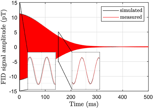
Figure 4. Comparison of simulated and measured FID signals for dephasing in the static field B0=38.6 μT and the gradient dBx/dx=2.4 μT/m. The insets show close ups from 0 to 1 ms and from 150 to 151 ms, respectively, and reveal a small field drift of ~15 nT in the measured FID compared to the simulation which assumes a constant Bx(r).
Phantom dcNCI experiments were then simulated for dipole depths of 15 and 35 mm representing a shallow and a deep cortical source, respectively. The voxel sizes were isotropic ranging from 5 to 25 mm.
We first present the results of the FEM calculations of the internal and external fields. In Figure 5, the magnetic field generated by the single dipole and the dipole grid within the phantom are shown for an applied current of 5 μA. Compared to the single dipole, the maximum field per unit current produced by the extended dipole is significantly smaller due to cancellation effects within the array. The simulations also show that cross currents in the grid phantom are effectively suppressed by the holes in the mounting plate facilitating the current flow across the grid.
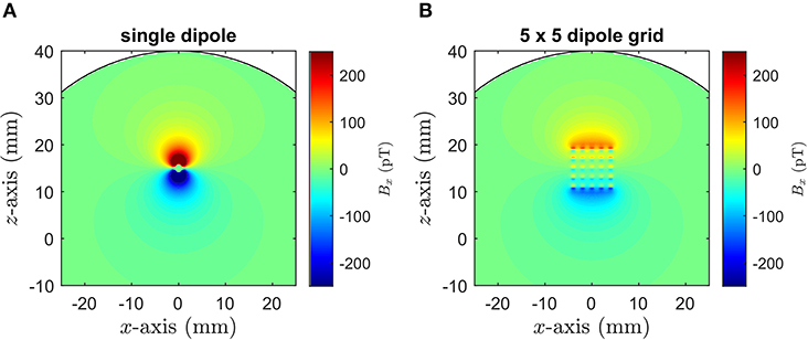
Figure 5. FEM simulation of the internal Bx field maps obtained for an applied current of 5 μA for (A) the single dipole and (B) the 5 × 5 dipole grid. The electrodes are parallel to the y-direction with the single dipole and the center of the dipole grid 15 mm above the spherical phantom center.
The calibration of the phantoms was carried out using the simulated and measured field distributions Bz/I outside the phantoms, as illustrated in Figure 6. The field generated by the extended dipole per unit current is 5% larger compared to the single dipole. The ECD reconstruction assumes a point-like dipole within a homogeneous conducting sphere. In case of the simulated data, the center of the sphere was set to −70 mm (with respect to the bottom of the sensor array) and the position of the dipole to 15 mm above it, as given by the geometry of the computational models.
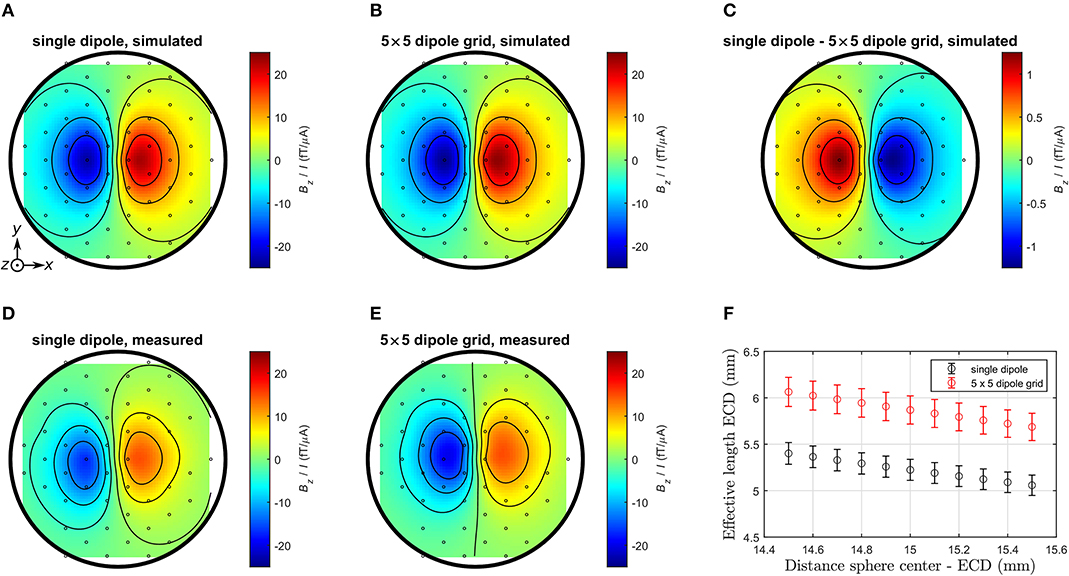
Figure 6. Comparison of simulated and averaged measured field maps obtained for the bottom sensor array of the 304-channel system. (A) Simulation single dipole. (B) Simulation 5 × 5 dipole grid. (C) Simulation single dipole − 5 × 5 dipole grid. (D) Measurement single dipole. (E) Measurement 5 × 5 dipole grid. (F) Fitted effective length of each dipole source for different distances ECD—sphere center. Circles denote the coordinates of the z-sensors. For the simulated data, all 304 channels were used for the reconstruction. For the measured data, 97 channels were deployed and complete coverage of the bottom z-plane was not possible, as some were malfunctioning.
For the measured maps, five fitting parameters were used: the coordinates of the sphere center relative to the bottom plane of the sensor array and the ECD components in x- and y-direction (zero z-component was imposed, as the alignment was defined by the phantom geometry). The estimated uncertainty of the ECD's vertical position of 0.5 mm was taken into account by performing source reconstructions for fixed distances in the range of (15 ± 0.5) mm. The resulting effective dipole lengths (ECD normalized by applied current) are shown in Table 3. The uncertainties are derived from the standard deviation of the fit parameters combined with the uncertainty of the dipole distance to the sphere center, as shown in Figure 6F.
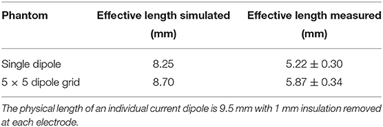
Table 3. Simulated and measured effective dipole lengths of the two phantoms.
The simulated effective lengths of the dipoles were found to be about 10% smaller than the physical dimension of the dipole electrodes. This is in line with expectations, as the current in the electrodes flows into the solution as soon as it reaches the uninsulated element of the Pt wire. Also, the effective length of the extended dipole is slightly larger than the single dipole both in the simulation and the measurement. The disagreement of about 30% compared to the actual values arises from an insufficient electric insulation of the current feeds on the PCB immersed in the aqueous solution. Due to this shunting, some of the current does not flow over the electrodes resulting in a reduced effective length of the physical dipoles.
We next present the results of the simulated noise-free dcNCI experiments considering 35 mm deep dipoles. In Figure 7A, the amplitude image together with the difference images are shown for the single dipole and the dipole grid for an ECDmax of 41 and 43 nAm, respectively. Also shown are experiments for a voxel size of 25 mm in Figure 7B, which were obtained for a dipole current of 80 μA corresponding to an ECDmax of 418 and 497 nAm for the single dipole and the dipole grid, respectively. The images have been phase adjusted to obtain the maximum difference signal ΔSmax. While the original location of the single dipole and the dipole grid center was z=0 for all voxel sizes, this adjustment shifts the dipole positions toward the voxel edge along +z. In this way, signal loss due to cancellation effects within one voxel is minimized.
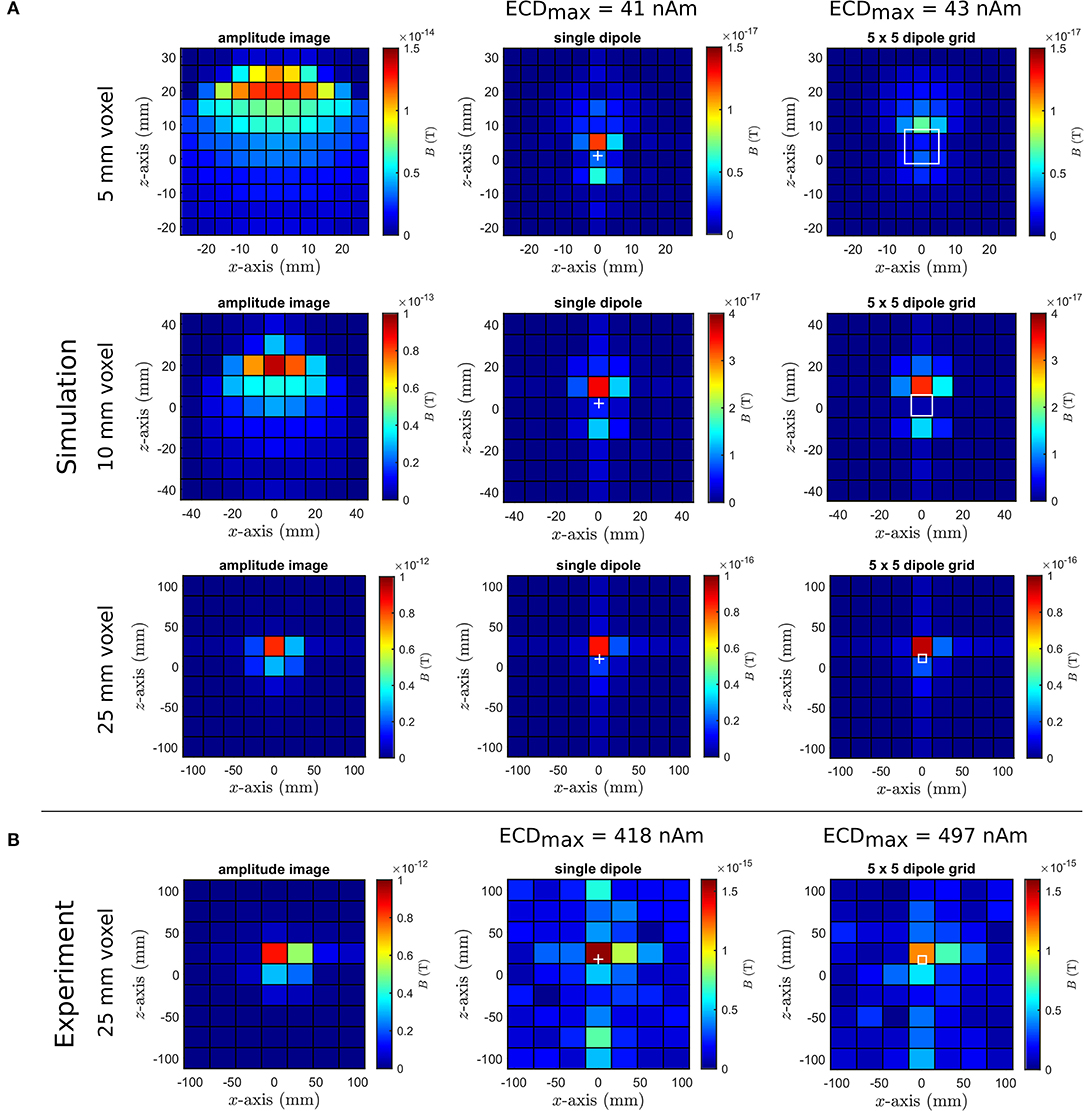
Figure 7. (A) Noise-free dcNCI simulations with voxel size of 5 mm (top), 10 mm (middle), and 25 mm (bottom) for 35 mm deep dipoles. Images were phase adjusted to obtain maximum ΔSmax which increases with voxel size; only for 5 mm is there a significant difference between the single dipole and the dipole grid. (B) Phantom experiments with nearly isotropic voxel size of 25 mm (Δx≈28 mm) and ~10× stronger ECDmax to enable clear identification of dipole activity in the presence of noise and artifacts. In all cases, amplitude images of the phantoms are shown on the left, difference amplitude images of the single dipole in the middle and of the dipole grid on the right. The cross and square denote the position of the single dipole and the dipole grid, respectively.
The maximum amplitude of the difference image ΔSmax is about 1,000 times smaller than the maximum amplitude image itself in agreement with previous NMR phantom studies [18]. As expected from the simulations of the phantom's internal field, ΔSmax of the single dipole is about a factor of 1.7 larger compared to the dipole grid for the 5 mm voxel size. The effect is most pronounced around the dipole where BDip is largest and the difference image appears smoother and more extended for the dipole grid. This effect disappears for voxel sizes larger than 10 mm and very similar ΔSmax are determined. Clearly, larger voxel sizes cannot reflect the detailed structure of the internal fields between the single dipole and the dipole grid. The phantom experiments for 25 mm voxel size reasonably reproduce the simulations with a twice as large expected ΔSmax for the single dipole. Good agreement is found for the dipole grid in this particular measurement. However, also visible are residual artifacts that could not be removed by the post-processing procedure (see Appendix for details).
The dependency of ΔSmax on the voxel size for dipole depths of 15 and 35 mm, as determined by the simulations, is displayed in Figure 8A. ΔSmax decreases with larger depth according to the sensitivity profile of the sensor system. In addition, ΔSmax increases linearly with voxel size up to about 15 mm and then levels off, which is particularly clear for the 35 mm deep dipoles. Also included is the image noise which reflects the sensitivity of the MRI setup for the image sequence using a phase encoding time of 30 ms. Figure 8A suggests that a 15 mm deep dipole with a maximum strength of 50 nAm could be theoretically detected by the low-noise MRI setup using the defined imaging sequence for voxel sizes >20 mm. In contrast, a 35 mm deep dipole would be unresolvable even for the largest voxel sizes, and we note that there is no significant difference between the single and the extended dipole source. Only for voxel sizes comparable to the physical dimensions of the dipolar source does the single dipole show a larger ΔSmax compared to the dipole grid, as already mentioned before.
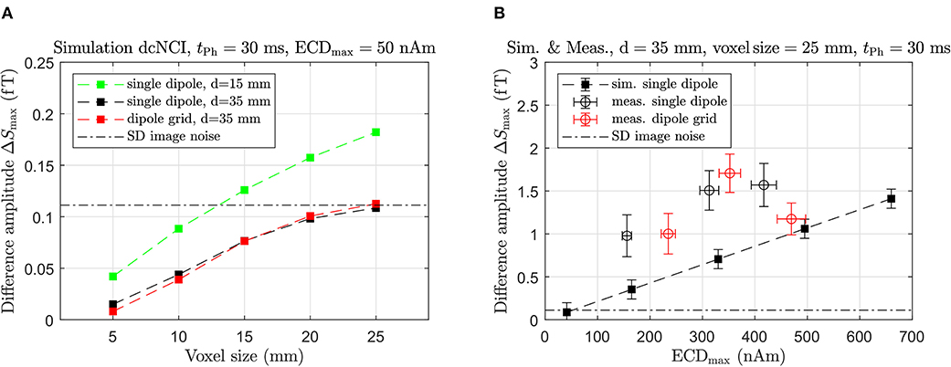
Figure 8. (A) Noise-free simulation of dcNCI showing ΔSmax in dependence of voxel size for the single dipole and the dipole grid with an ECDmax of 50 nAm and different depths. (B) Comparison between simulated and measured ΔSmax vs. ECDmax.
Figure 8B shows the dependence of ΔSmax on the applied ECDmax for dipoles at a fixed depth of 35 mm and a voxel size of 25 mm. The simulations predict, that the amplitude of the difference signal decreases linearly with a decreasing current dipole strength in line with previous NMR phantom studies [18]. For the experimental data, ΔSmax and the SD are factor of ~2 larger than predicted by the simulations. We attribute both effects to the aforementioned residual artifacts and discuss this in more detail later.
The results of the simulations and measurements indicate that a 35 mm deep dipole with an ECDmax of about 150 nAm could be resolved using voxel sizes not smaller than 25 mm. Therefore, the detection of a realistic current dipole strength of 50 nAm requires an improvement of the experimental sensitivity by at least a factor of 3.
In order to identify optimal dcNCI sequence parameters for maximum CNR, multiple images were simulated varying the phase time tPh from 15 to 100 ms corresponding to echo times tE of 30 to 200 ms for the 1st echo. The gradients GF and GPh, max were adjusted accordingly to obtain a voxel size of 25 mm, as illustrated in Figure 3, while the number of phase encoding steps was fixed with Ny = Nz=10 retaining the FOVy, z of 25 cm. Since the sampling frequency was kept constant and tDet depends on tPh, the FOVx varied, but was in the meter-range in all cases.
An optimum sequence is expected, as two competing mechanisms occur. A longer tE allows BDip to cause larger frequency shifts, but, on the other hand, spin relaxation leads to a signal decrease. As BDip is not constant and derived from an actual MEG measurement, comprehensive simulations are required to determine an optimal tPh. For comparison, the optimization was also carried out for a true DC activity, which may be elicited for instance by auditory stimulation [34]. We reiterate that this is in contrast to conventional imaging where tPh should be as short as possible to obtain maximum image SNR. We also limit this optimization to an inverted frequency encoding gradient GF during echo formation so that tDet = 2tPh as this is implemented in our hardware. Application of a different GF during this period would allow one to vary tDet independently from tPh.
In Figure 9, the dependencies of ΔSmax and the CNR, both normalized by ECDmax, on the echo time tE are illustrated. The normalization allows the comparison of the predictions between the realistic sustained MEG activity and a constant DC signal. Since four echoes were simulated for each phase time, different tPh result on occasion in an identical tE for different echoes. As shown in Figure 3, for example, the 2nd echo of a sequence with tPh is formed at the same time as the 1st echo when resulting in equal echo peak amplitudes. Hence, the values for ΔSmax collapse for separate echoes provided the echo times are the same. The DC signal results in a larger normalized ΔSmax and the maximum values are observed for an echo time of ~90 and 120 ms for the MEG and the DC signal, respectively.
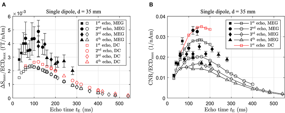
Figure 9. (A) Dependency of ΔSmax/ECDmax and (B) CNR/ECDmax for varying echo times tE and a voxel size of 25 mm. Open markers represent noise-free simulations and filled markers phantom experiments using 80 μA. Results are grouped according to echo number and an example for data belonging to tPh=15 ms are connected by the dashed black line in (B).
The experimental results were obtained with a dipole current of 80 μA. Again, they show values for ΔSmax/ECDmax about a factor of 2 larger than the predictions; however, they also clearly demonstrate the maximum at tE~100 ms in line with the simulations.
The CNR, on the other hand, shows an optimum at tE~150 ms both for the sustained MEG and the constant DC signal, respectively (see Figure 9B). In explaining this result, we refer again also to Figure 3. In our sequence we always have tDet = 2tPh and for a given echo, an increase in tPh, and correspondingly tE, leads to a longer acquisition time tDet. For the 1st echo, for instance, this gives tDet = tE. Since the sampling frequency is kept constant, the noise is then distributed over more frequency bins resulting in . Beyond tE resulting in maximum ΔSmax, the image noise decreases more strongly compared to ΔSmax pushing the optimum for CNR to longer echo times. The maxima are rather broad and, as ΔSmax/ECDmax is smaller for the MEG-derived signal, its CNR is correspondingly decreased. The maximum CNR for each echo occurs at the same echo time but decreases for consecutive echoes as tDet gets successively shorter and consequently the noise larger, as discussed above. This is not shown for the true DC signal which exhibits the same behavior. For large tE, spin relaxation dominates causing ΔSmax and CNR to approach zero eventually.
The enhancement in CNR compared to the experimental setup when using a tE of 60 ms is a factor of 1.5 for the MEG signal improving the detection limit from ~150 to 100 nAm. A true DC activation in comparison to the MEG-derived activity results in an even better improvement of 1.85 provided it has the same ECDmax. The phantom experiments confirm this picture and, within the accuracy of the measurement, the maximum in CNR at tE~150 ms is also observed. It is worth pointing out that increasing tE from 60 to 150 ms has only a secondary effect on the total measurement time, since this is dominated by the polarizing time tP, in particular if only the 1st echo is acquired.
A comparison between simulated and measured 3D dcNCI phantom experiments show an approximately 2-fold larger ΔSmax for the experimental case. In the simulation model, we used independently determined quantities, e.g., SQUID conversion factor, and the actual geometry of the phantom within idealized MRI fields without any freely adjustable parameter. The very good agreement in the validation measurement of the solver (see Figure 4) confirms the accuracy of the computational model. However, with this in mind, the generally larger effect in the 3D dcNCI phantom experiments deserves a closer inspection. It is possibly related to the increased uncertainty due to residual artifacts, which—as pointed out in the Appendix—are likely due to field drifts of environmental origin within the moderately shielded MSR that are undetectable by the sensing circuit. This might introduce a bias toward an overestimation of ΔSmax. Clearly, the residual artifacts after subtraction represent an experimental issue and a more strongly shielded environment may provide a possible solution. As a further comment, we consider an erroneous determination of the ECDmax of the phantoms unlikely, since the observed shunting during the calibration proved to be stable in time. Further studies are required to determine the origin of the larger experimental ΔSmax. Nevertheless, we consider the agreement adequate and the results of the simulations form the basis for further discussions below.
As we have shown, the theoretical CNR of 3D dcNCI using voxel sizes in the cm-range and an optimized sequence applied to our low-noise ULF-MRI setup is only slightly larger than unity. In addition, compared to the phantoms, the water content of brain tissue is lower and heterogeneous ranging from 70.6% for white matter, 84.3% for gray matter and 97.5% for cerebrospinal fluid (CSF) [35]. Partial volume effects may then be present as large voxel sizes are likely to include multiple tissues. Consequently, one can expect a reduction in CNR in an in vivo experiment which depends on the size and the location of each voxel and for the present discussion, we assume a worst case value of 70.6%. However, improvements are possible on the instrumental side. We performed the study for a moderate BP of 17 mT, the maximum achievable field of our setup. A much larger BP of up to 150 mT has been demonstrated in in vivo imaging of the human brain [3] corresponding to an increase in M0 and consequently in ΔSmax of a factor 9.
With respect to the noise performance, the application of a large BP has been shown to lead to an excess low-frequency noise due to flux trapping in the superconducting pick-up coil [36]. However, it may be avoided by operation at a sufficiently large Larmor frequency [37], a suitable BP ramp down [38] or rapid thermal cycling of the pick-up coil [39]. Consequently, the noise performance is ultimately limited by Johnson noise of the human body which was recently measured at 55 aTHz−1/2 [40]. Improvements in SQUID performance, e.g., by use of sub-micron-sized Josephson junctions, lead us then to the conclusion that a noise level of about 100 aTHz−1/2, although being quite challenging, is nevertheless feasible [41, 42]. Of course, this discussion requires instrumental factors, such as noise generated by the field and gradient supplies to be negligible, as should be the case for our ULF-MRI setup. In addition, the occurrence of artifacts will have to be addressed. The projected CNR for the MEG-derived sustained activity with ECDmax=50 nAm and all these factors taken into account is shown in Figure 10.
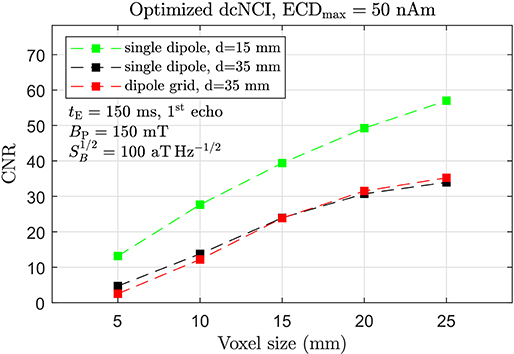
Figure 10. Projected CNR for optimized dcNCI of the MEG-derived sustained activity with an ECDmax of 50 nAm taking tE=150 ms (1st echo), BP=150 mT, and 100 aT Hz−1/2. Signal reduction by 0.706 due to reduced spin density was taken into account.
An overall improvement of ~35 in CNR for the optimized dcNCI setup appears possible. With CNR ~10, a 15 mm deep, shallow focal cortical source should be well resolvable with a voxel size of ~5 mm. For deeper sources, such as the exemplary somatosensory evoked sustained activity, the voxel size for CNR~10 is about 10 mm. Voxel sizes in the range of 5 mm result again in CNR close to unity and represent in our opinion the theoretical limit of 3D dcNCI.
The development of a validated computational framework, able to execute virtual dcNCI experiments, was motivated by multiple needs. The identification of the required technological improvements of ULF-MR hardware and the identification of optimized dcNCI sequence parameters being the most prominent. In particular, a sound knowledge of the impact of the neuronal source spatial distribution, timing and orientation on the MR signals permits the identification of optimal strategies for detection. Hardware measures, such as increase of BP and the reduction of system noise, are rather obvious means to improve the CNR for the realization of dcNCI.
In assessing the relevance of the experimental and computational phantom study for in vivo dcNCI, several issues are worth discussing. dcNCI using ULF MRI, as presented here, is limited to evoked and sustained, ideally monophasic, neuronal activities. In addition, the emphasis is on focal activation which can be approximated, at least from an MEG point of view, by a dipolar source and parameterized by an ECD. In this case, the simulation studies show that for voxel sizes larger than 10 mm there is no significant difference between the single dipole and the extended dipole grid in sensitivity even though the internal fields are markedly different. This suggests, that the detailed spatial structure of the neuronal field in an in vivo experiment cannot be resolved by 3D dcNCI for voxel sizes larger than 10 mm and voxels in the low mm-range are needed to possibly achieve this.
The dependence on sustained activities of dcNCI has also bearing on the temporal resolution which is of the order of the echo time tE, the time during which the long-lasting activity is present. For the somatosensory evoked and a true DC activation, this amounts to 120 ms for the optimized sequence which is significantly longer than in MEG but superior to fMRI. Note that this comparison relates to the time needed to acquire one line in k-space and not the entire image, which is much longer. This emphasizes again the limitation to evoked activities that can be elicited reliably. By reducing tE, an improvement of the temporal resolution at the expense of CNR is possible.
A further point which deserves attention is the requirement of parallel alignment between BDip and B0 in order to result in a maximum CNR. However, this condition is less restrictive than it might first appear. As long as B0≫BDip, which is certainly fulfilled even for dcNCI using ULF MRI, the component of BDip parallel to B0 is of significance. As this scales as cosϕ, where ϕ is the angle between B0 and BDip, even a substantial misalignment by ϕ=30°, for example, results in a reduction of the CNR by only ~13%. As a corollary we note that a radial dipole, although silent in MEG, will show the full effect in dcNCI as long as the dipole is perpendicular B0.
Finally, the above estimation of the sensitivity limit was based on the assumption of a homogeneous distribution of white-matter-like tissue within the MRI voxel. However, as already mentioned, single voxel signals are expected to be largely influenced by partial volume effects due to the presence of multiple tissues with different proton densities and relaxation times, such as white matter, CSF, bone, dura, and blood vessels. This and many other concomitant factors, related to the complex anatomical and neuroelectric complexity of the human head, have not been investigated in this work. This could be done replacing simplified phantom models with high-resolution anatomical human head models, such as the ones of the Virtual Population (IT'IS Foundation, Zurich, Switzerland) [43] or the MIDA head model [44], combined with realistic electrophysiological models of neuronal networks.
In conclusion, we illustrated the elements of a validated computational framework allowing virtual experiments with the aim to assess the feasibility of 3D dcNCI. The simulations provide a controllable basis which allows the evaluation for a best-case scenario. To this end, we considered idealized MRI fields and magnetic field distributions generated by current dipole phantoms mimicking neuronal activities. The source models consisted of a single dipole and an extended dipole grid with well-defined phantom geometry enabling accurate FEM simulations of the internal and the external fields. The latter were validated with MEG-type measurements, which served as a calibration of the fabricated phantoms. An MR solver based on an analytical solution to the Bloch equation was developed and used to simulate the dcNCI experiment based on our low-noise 3D ULF-MRI setup. The framework was verified via phantom experiments and allowed the assessment of the detection limit. This experimental part was equally important, since it highlights the technical challenges which need to be addressed.
We found that with our current technology and an optimized dcNCI sequence minimal voxel sizes of 20 mm are required to detect a 35 mm dipole deep dipole with an ECD of about 100 nAm, which is a factor of 2 larger than the physiological value. In addition, we used this tool to project a possible 35-fold increase in CNR due to hardware improvements. The framework should be combined with field simulations of a realistic neuronal network embedded inside a cortical structure. This is highly desirable, as it would ultimately allow the optimization of in vivo dcNCI based on ULF MRI which remains a formidable challenge.
The raw data supporting the conclusions of this article will be made available by the authors, without undue reservation.
NH, AC, and RK contributed to the conception of the study. J-HS developed the dipole phantoms and performed the FEM simulations. NH performed the dcNCI phantom experiments, analyzed the dcNCI data, and wrote the first draft of the manuscript. RK developed the MR solver and revised the manuscript based on the annotations of the co-authors. PH contributed to system performance. All authors contributed to manuscript revision, read, and approved the submitted version.
This project has received funding from the DFG under Grant KO 5321/1-1, the SNF under project No 200021E-166809, and from the European Union's Horizon 2020 research and innovation programme under grant agreement No 686865.
The authors declare that the research was conducted in the absence of any commercial or financial relationships that could be construed as a potential conflict of interest.
The Supplementary Material for this article can be found online at: https://www.frontiersin.org/articles/10.3389/fphy.2021.647376/full#supplementary-material
1. Greenberg YS. Application of superconducting quantum interference devices to nuclear magnetic resonance. Rev Modern Phys. (1998) 70:175–222. doi: 10.1103/RevModPhys.70.175
2. de Souza RE, Schlenga K, Wong-Foy A, McDermott R, Pines A, Clarke J. NMR and MRI obtained with high transition temperature dc SQUIDs. J Brazil Chem Soc. (1999) 10:307–12. doi: 10.1590/S0103-50531999000400009
3. Inglis B, Buckenmaier K, SanGiorgio P, Pedersen AF, Nichols MA, Clarke J. MRI of the human brain at 130 microtesla. Proc Natl Acad Sci USA. (2013) 110:19194–201. doi: 10.1073/pnas.1319334110
4. Zotev VS, Matlashov AN, Volegov PL, Savukov IM, Espy MA, Mosher JC, et al. Microtesla MRI of the human brain combined with MEG. J Magn Reson. (2008) 194:115–20. doi: 10.1016/j.jmr.2008.06.007
5. Lee SJ, Shim JH, Kim K, Yu KK, Hwang Sm. Magnetic resonance imaging without field cycling at less than earth's magnetic field. Appl Phys Lett. (2015) 106:103702. doi: 10.1063/1.4914973
6. Vesanen PT, Nieminen JO, Zevenhoven KCJ, Dabek J, Parkkonen LT, Zhdanov AV, et al. Hybrid ultra-low-field MRI and magnetoencephalography system based on a commercial whole-head neuromagnetometer. Magn Reson Med. (2013) 69:1795–804. doi: 10.1002/mrm.24413
7. Hilschenz I, Körber R, Scheer HJ, Fedele T, Albrecht HH, Cassará AM, et al. Magnetic resonance imaging at frequencies below 1 kHz. Magn Reson Imaging. (2013) 31:171–7. doi: 10.1016/j.mri.2012.06.014
8. Espy M, Volegov P, Matlachov AN, George J, Kraus RH Jr. Simultaneously detected biomagnetic signals and NMR. Neurol Clin Neurophysiol. (2004) 2004:12.
9. Babiloni C, Pizzella V, Del Gratta C, Ferretti A, Romani GL. Fundamentals of electroencefalography, magnetoencefalography, and functional magnetic resonance imaging. Int Rev Neurobiol. (2009) 86:67–80. doi: 10.1016/S0074-7742(09)86005-4
10. Singh M. Sensitivity of MR phase shift to detect evoked neuromagnetic fields inside the head. IEEE Trans Nucl Sci. (1994) 41:349–51. doi: 10.1109/23.281521
11. Song AW, Takahashi AM. Lorentz effect imaging. Magn Reson Imaging. (2001) 19:763–7. doi: 10.1016/S0730-725X(01)00406-4
12. Witzel T, Lin FH, Rosen BR, Wald LL. Stimulus-induced Rotary Saturation (SIRS): a potential method for the detection of neuronal currents with MRI. Neuroimage. (2008) 42:1357–65. doi: 10.1016/j.neuroimage.2008.05.010
13. Parkes LM, de Lange FP, Fries P, Toni I, Norris DG. Inability to directly detect magnetic field changes associated with neuronal activity. Magn Reson Med. (2007) 57:411–6. doi: 10.1002/mrm.21129
14. Chu R, de Zwart JA, van Gelderen P, Fukunaga M, Kellman P, Holroyd T, et al. Hunting for neuronal currents: absence of rapid MRI signal changes during visual-evoked response. Neuroimage. (2004) 23:1059–67. doi: 10.1016/j.neuroimage.2004.07.003
15. Mößle M, Han SI, Myers WR, Lee SK, Kelso N, Hatridge M, et al. SQUID-detected microtesla MRI in the presence of metal. J Magn Reson. (2006) 179:146–51. doi: 10.1016/j.jmr.2005.11.005
16. Kraus RH, Volegov P, Matlashov AN, Espy M. Toward direct neuronal current imaging by resonant mechanisms at ultra-low field. Neuroimage. (2007) 39:310–7. doi: 10.1016/j.neuroimage.2007.07.058
17. Höfner N, Albrecht HH, Cassará AM, Curio G, Hartwig S, Haueisen J, et al. Are brain currents detectable by means of low-field NMR? A phantom study. Magn Reson Imaging. (2011) 29:1365–73. doi: 10.1016/j.mri.2011.07.009
18. Körber R, Nieminen JO, Höfner N, Jazbinšek V, Scheer HJ, Kim K, et al. An advanced phantom study assessing the feasibility of neuronal current imaging by ultra-low-field NMR. J Magn Reson. (2013) 237:182–90. doi: 10.1016/j.jmr.2013.10.011
19. Kim K, Lee SJ, Kang CS, Hwang Sm, Lee YH, Yu KK. Toward a brain functional connectivity mapping modality by simultaneous imaging of coherent brain waves. Neuroimage. (2014) 91:63–9. doi: 10.1016/j.neuroimage.2014.01.030
20. Cassarà AM, Hagberg GE, Bianciardi M, Migliore M, Maraviglia B. Realistic simulations of neuronal activity: a contribution to the debate on direct detection of neuronal currents by MRI. Neuroimage. (2008) 39:87–106. doi: 10.1016/j.neuroimage.2007.08.048
21. Konn D, Gowland P, Bowtell R. MRI detection of weak magnetic fields due to an extended current dipole in a conducting sphere: a model for direct detection of neuronal currents in the brain. Magn Reson Med. (2003) 50:40–9. doi: 10.1002/mrm.10494
22. Xue Y, Gao JH, Xiong J. Direct MRI detection of neuronal magnetic fields in the brain: theoretical modeling. Neuroimage. (2006) 31:550–9. doi: 10.1016/j.neuroimage.2005.12.041
23. Park TS, Lee SY. Effects of neuronal magnetic fields on MRI: numerical analysis with axon and dendrite models. Neuroimage. (2007) 35:531–8. doi: 10.1016/j.neuroimage.2007.01.001
24. Blagoev KB, Mihaila B, Travis BJ, Alexandrov LB, Bishop AR, Ranken D, et al. Modelling the magnetic signature of neuronal tissue. Neuroimage. (2007) 37:137–48. doi: 10.1016/j.neuroimage.2007.04.033
25. Luo Q, Jiang X, Chen B, Zhu Y, Gao JH. Modeling neuronal current MRI signal with human neuron. Magn Reson Med. (2011) 65:1680–9. doi: 10.1002/mrm.22764
26. Körber R, Storm JH, Seton H, Mäkelä JP, Paetau R, Parkkonen L, et al. SQUIDs in biomagnetism: a roadmap towards improved healthcare. Supercond Sci Technol. (2016) 29:113001. doi: 10.1088/0953-2048/29/11/113001
27. Hömmen P, Storm JH, Höfner N, Körber R. Demonstration of full tensor current density imaging using ultra-low field MRI. Magn Reson Imaging. (2019) 60:137–44. doi: 10.1016/j.mri.2019.03.010
28. Voigt J, Knappe-Grüneberg S, Gutkelch D, Haueisen J, Neuber S, Schnabel A, et al. Development of a vector-tensor system to measure the absolute magnetic flux density and its gradient in magnetically shielded rooms. Rev Sci Instrum. (2015) 86:055109. doi: 10.1063/1.4921583
29. Storm JH, Hömmen P, Drung D, Körber R. An ultra-sensitive and wideband magnetometer based on a superconducting quantum interference device. Appl Phys Lett. (2017) 110:072603. doi: 10.1063/1.4976823
30. Körber R. Ultra-sensitive SQUID instrumentation for MEG and NCI by ULF MRI. In: EMBEC & NBC 2017. Singapore: Springer Singapore (2017). p. 795–8. doi: 10.1007/978-981-10-5122-7_199
31. Zotev VS, Matlashov AN, Savukov IM, Owens T, Volegov PL, Gomez JJ, et al. SQUID-based microtesla MRI for in vivo relaxometry of the human brain. IEEE Trans Appl Supercond. (2009) 19:823–6. doi: 10.1109/TASC.2009.2018764
32. Schnabel A, Burghoff M, Hartwig S, Petsche F, Steinhoff U, Drung D, et al. A sensor configuration for a 304 SQUID vector magnetometer. Neurol Clin Neurophysiol. (2004) 2004:70.
33. Burghoff M, Albrecht HH, Hartwig S, Hilschenz I, Körber R, Sander Thömmes T, et al. SQUID system for MEG and low field magnetic resonance. Metrol Meas Syst. (2009) 16:371–6.
34. Keceli S, Inui K, Okamoto H, Otsuru N, Kakigi R. Auditory sustained field responses to periodic noise. BMC Neurosci. (2012) 13:7. doi: 10.1186/1471-2202-13-7
35. Mansfield P. Imaging by nuclear magnetic resonance. J Phys E Sci Instrum. (1988) 21:18–30. doi: 10.1088/0022-3735/21/1/002
36. Storm JH, Drung D, Burghoff M, Körber R. A modular, extendible and field-tolerant multichannel vector magnetometer based on current sensor SQUIDs. Supercond Sci Technol. (2016) 29:094001. doi: 10.1088/0953-2048/29/9/094001
37. Espy MA, Magnelind PE, Matlashov AN, Newman SG, Sandin HJ, Schultz LJ, et al. Progress toward a deployable SQUID-based ultra-low field MRI system for anatomical imaging. IEEE Trans Appl Supercond. (2015) 25:1–5. doi: 10.1109/TASC.2014.2365473
38. Al-Dabbagh E, Storm JH, Körber R. Ultra-sensitive SQUID systems for pulsed fields—degaussing superconducting pick-up coils. IEEE Trans Appl Supercond. (2018) 28:1–5. doi: 10.1109/TASC.2018.2797544
39. Matlashov A, Magnelind P, Volegov P, Espy M. Elimination of 1/f noise in gradiometers for SQUID-based ultra-low field nuclear magnetic resonance. In: 2015 15th International Superconductive Electronics Conference (ISEC). Nagoya (2015). p. 1–3. doi: 10.1109/ISEC.2015.7383455
40. Storm JH, Hömmen P, Höfner N, Körber R. Detection of body noise with an ultra-sensitive SQUID system. Meas Sci Technol. (2019) 30:125103. doi: 10.1088/1361-6501/ab3505
41. Körber R, Kieler O, Hömmen P, Höfner N, Storm J. Ultra-sensitive SQUID systems for applications in biomagnetism and ultra-low field MRI. In: 2019 IEEE International Superconductive Electronics Conference (ISEC). Riverside, CA (2019). p. 1–3. doi: 10.1109/ISEC46533.2019.8990912
42. Storm JH, Kieler O, Körber R. Towards ultrasensitive SQUIDs based on submicrometer-sized Josephson junctions. IEEE Trans Appl Supercond. (2020) 30:1–5. doi: 10.1109/TASC.2020.2989630
43. Gosselin MC, Neufeld E, Moser H, Huber E, Farcito S, Gerber L, et al. Development of a new generation of high-resolution anatomical models for medical device evaluation: the Virtual Population 3.0. Phys Med Biol. (2014) 59:5287–303. doi: 10.1088/0031-9155/59/18/5287
Keywords: ultra-low-field magnetic resonance imaging, neuronal current imaging, current dipole phantom, MEG, simulation
Citation: Höfner N, Storm J-H, Hömmen P, Cassarà AM and Körber R (2021) Computational and Phantom-Based Feasibility Study of 3D dcNCI With Ultra-Low-Field MRI. Front. Phys. 9:647376. doi: 10.3389/fphy.2021.647376
Received: 29 December 2020; Accepted: 18 March 2021;
Published: 26 April 2021.
Edited by:
Mathieu Sarracanie, University of Basel, SwitzerlandReviewed by:
Angelo Galante, University of L'Aquila, ItalyCopyright © 2021 Höfner, Storm, Hömmen, Cassarà and Körber. This is an open-access article distributed under the terms of the Creative Commons Attribution License (CC BY). The use, distribution or reproduction in other forums is permitted, provided the original author(s) and the copyright owner(s) are credited and that the original publication in this journal is cited, in accordance with accepted academic practice. No use, distribution or reproduction is permitted which does not comply with these terms.
*Correspondence: Rainer Körber, cmFpbmVyLmtvZXJiZXJAcHRiLmRl
Disclaimer: All claims expressed in this article are solely those of the authors and do not necessarily represent those of their affiliated organizations, or those of the publisher, the editors and the reviewers. Any product that may be evaluated in this article or claim that may be made by its manufacturer is not guaranteed or endorsed by the publisher.
Research integrity at Frontiers
Learn more about the work of our research integrity team to safeguard the quality of each article we publish.