Time-Varying Volatility in Bitcoin Market and Information Flow at Minute-Level Frequency

In this article, we analyze the time series of minute price returns on the Bitcoin market through the statistical models of the generalized autoregressive conditional heteroscedasticity (GARCH) family. We combine an approach that uses historical values of returns and their volatilities—GARCH family of models, with a so-called Mixture of Distribution Hypothesis, which states that the dynamics of price returns are governed by the information flow about the market. Using time series of Bitcoin-related tweets, the Bitcoin trade volume, and the Bitcoin bid–ask spread, as external information signals, we test for improvement in volatility prediction of several GARCH model variants on a minute-level Bitcoin price time series. Statistical tests show that GARCH(1,1) and cGARCH(1,1) react the best to the addition of external signals to model the volatility process on out-of-sample data.

1 Introduction

The first mathematical description of the evolution of price changes in a market dates back to Bachelier [1] (later rediscovered as Brownian motion, or random walk model), Mandelbrot [2] (price increments are Lévy stable distribution), and truncated Lévy processes [3]. An opposing hypothesis (later named “Mixture of Distribution Hypothesis”) was introduced by Clark [4], where the non-normality of price returns distribution is assigned to the varying rate of price series evolution during different time intervals. The process that is driving the rate of price evolution is proposed to be the information flow available to the traders. Due to the governing of the information flow, the number of summed price changes per observed time interval varies substantially, and the central limit theorem cannot be applied to obtain the distribution of price changes. Nevertheless, a generalization of the theorem provides a Gaussian limit distribution conditional on the random variable directing the number of changes [4]. In a different approach, the autoregressive conditional heteroscedasticity (ARCH) [5] model, originally introduced by Engle, describes the heteroscedastic behavior (time-varying volatility) of logarithmic price returns relying only on the information of previous price movements. In addition to the previous values of price returns, its generalized variant GARCH [6] introduces previous conditional variances as well when calculating the present conditional variance. GARCH is thus able to account for volatility clustering and for the leptokurtic distribution of price returns, both the stylized statistical properties of returns. An alternative view comes from the GARCH-Jump model [7], which assumes that the news process can be represented as ${\mathit{ϵ}}_t={\mathit{ϵ}}_{1,t}+{\mathit{ϵ}}_{2,t}$, a superposition of a normal component ${\mathit{ϵ}}_{1,t}={\sigma }_t{z}_t$ and a jump-like Poisson component with intensity λ. The constant intensity was generalized to autoregressive conditional jump intensity ${\lambda }_t=f\left({\lambda }_{t-1}\right)$ in [8].

Contrary to other studies about news jump dynamics and impact on daily returns [8, 9], we will model the volatility and external signals on a minute-level granularity. On this timescale, our external signals are not modeled with Poisson-like dynamics, but added directly as an exogenous observable variable $I_{t-1}$ to form GARCHX model.

In this article, we compare price volatility predictions of GARCH(1,1) with those of GARCHX (1,1) to explore how information is absorbed into the emerging cryptocurrency market of Bitcoin. The Bitcoin [10] is a cryptocurrency system operated through the peer-to-peer network nodes, with a publicly distributed ledger called blockchain [11]. Similar to the foreign exchange markets, Bitcoin markets [12, 13] allow the exchange to fiat currencies and back. Different studies on Bitcoin quantify the price formation [14, 15], bubbles [16, 17], volatility [18, 19], systems dynamics [20–22], and economic value [23–25]. Various studies [26–29] have used social signals from social media, WWW, search queries, sentiment, comments, and replies on forums, and [30] added information from the blockchain as an external signal to the GARCH model. Several models from the GARCH family have been used for modeling and forecasting of multiple cryptocurrencies [31, 32] on a daily level and IGARCH was shown to be superior to other models. Twitter data have been exploited to give successful daily [33] predictions on Bitcoin volume and volatility using only Twitter volume, and successful hourly predictions on returns and volatility with the added Twitter sentiment [34]. We focus this study on understanding Bitcoin volatility process and the statistical quantification of the predictive power of the class of GARCH models with exogenous signals from social media tweets, trading volume, and order book on a minute level timescale.

2 Data

We used two types of price definitions, the mid-quote price and the volume-weighted price, both calculated at a minute level. Mid-quote price was constructed as the average between the maximum bid and the minimum ask price on the last tick per minute, and the volume-weighted average price (VWAP) as the volume-weighted average of transaction prices per minute.

Sampling prices at such a high frequency brings up the issue of microstructure effects, such as bid–ask bounce, that introduces the autocorrelation between consecutive prices. Because of that, in addition to volume weighted prices, we use mid-quote prices that have a significantly smaller first order of autocorrelation, as explained in [35], to strengthen the robustness of the results. An autocorrelation plot for both types of price returns is shown in the Appendix.

The Bitcoin prices were obtained from the Bitfinex exchange, and logarithmic returns were calculated as a natural logarithm of two consecutive prices. The period we observed spans from April 18th, 2019, to May 30th, 2019, with 58,000 observations in total, 50,000 observations as in-sample, and 8,000 as out-of-sample, and is shown on Figure 1A. In the table in Figure 1B, we can see the descriptive statistics of both kinds of logarithmic returns; the mean values of the returns are very close to zero $\left(8\cdot {10}^{-6}\right)$, with standard deviations of $9.41\cdot {10}^{-4}$ and $9.94\cdot {10}^{-4}$, both distributions are negatively skewed and leptokurtic.

FIGURE 1

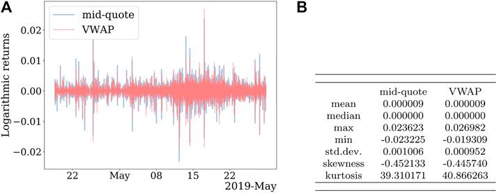
FIGURE 1. Volume-weighted and mid-quote logarithmic returns for the Bitcoin market. (A) Time series. (B) Descriptive statistics.

Three different datasets for external signals were available as the external information proxy—a time series of the number of tweets mentioning cryptocurrency-related news [36], a time series of Bitcoin trade volumes from Bitfinex market, and a time series of Bitcoin bid–ask spread, created as a time series of absolute differences between the maximum bid and the minimum ask price at every recorded instant, also from Bitfinex market. The data are collected on a second level and shown in Figures 2A–C, with the descriptive statistics in Figure 2D. All three time series were aggregated to the minute level. The data were not normalized.

FIGURE 2

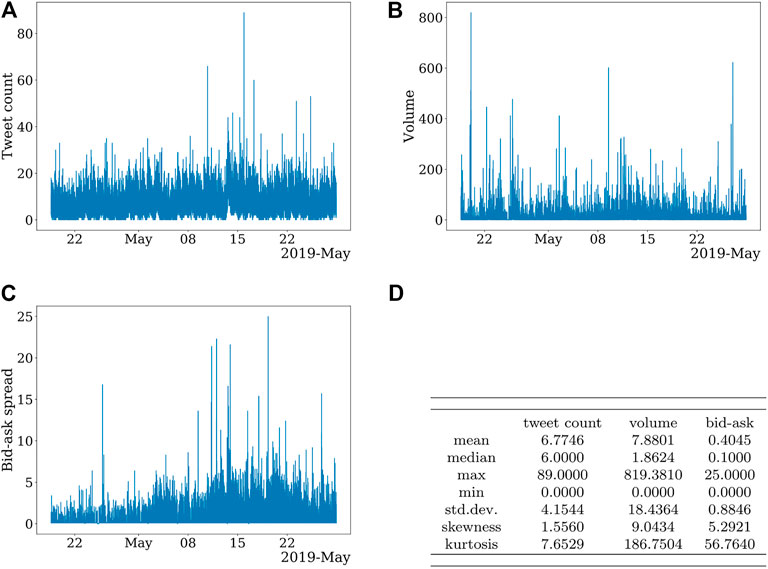
FIGURE 2. (A) Time series external signal of cryptocurrency-related tweets. (B) Time series of trading volume on Bitfinex market for BTC-USD pair. (C) Time series of bid–ask spread on Bitfinex market for BTC-USD pair. (D) Descriptive statistics of external signals for Bitcoin market.

3 Mixture of Distribution Hypothesis

The “Mixture of Distribution Hypothesis” models the non-normality of price returns distribution with the varying rate of price series evolution due to the different information flow during different time intervals. Practically, Clark [4] hypothesizes that this can be observed as a linear relationship between the proxy for the information flow $I_t$ and the price change variance $r_t^2$, and suggests trading volume $v_t$ as the proxy. Tauchen and Pitts [37] state a bivariate normal mixture model which conditions the price returns and trading volume on the information flow as:

$r_t={\displaystyle \sum _{i=1}^{I_t}{r}_{t,i}},r_{t,i}\in \mathcal{N}(0,{\sigma }_1).(1)$

$v_t={\displaystyle \sum _{i=1}^{I_t}{v}_{t,i}},v_{t,i}\in \mathcal{N}({\mu }_2,{\sigma }_2).(2)$

Both, the price return and trading volume are mixture of independent normal distributions with the same mixing variable $I_t$, which represents the number of new pieces of information arriving to market. Conditioned on $I_t$, price changes are distributed as $\mathcal{N}\left(0,I_t{\sigma }_1\right)$ and the trading volume is distributed as $\mathcal{N}\left(I_t{\mu }_2,I_t{\sigma }_2\right)$, and the model can be rewritten as:

$r_t={\sigma }_1\sqrt{I_t}{z}_{1t},z_{1t}\in N\left(\mathrm{0,1}\right).(3)$

$v_t={\mu }_2{I}_t+{\sigma }_2\sqrt{I_t}{z}_{2t},z_{2t}\in N\left(\mathrm{0,1}\right).(4)$

The relationship between price variance and trading volume immediately follows:

$Cov\left(r_t^2,v_t\right)={\sigma }_1{\mu }_{2}Var\left(I_t\right),(5)$

and the stochastic term in Eq. 4 shows that the above-proposed linear relationship is only an approximation.

To start our analysis, we calculated correlation plots for the relationship between the external signals and the squared VWAP price returns. The correlation between squared price returns and volume was calculated for different time lags of the volume time series, as shown in Figure 3A. Both have a peak when the external series leads the squared price returns by 1 min. The significant correlation, that is, normalized covariance between squared price returns and trading volume indicates an approximately linear relationship between the volatility and the two proxies for information flow (see Eq. 3). The result we got using the bid–ask spread as an external signal can be seen (Figure 3B) to be analogous to the one obtained for volume.

FIGURE 3

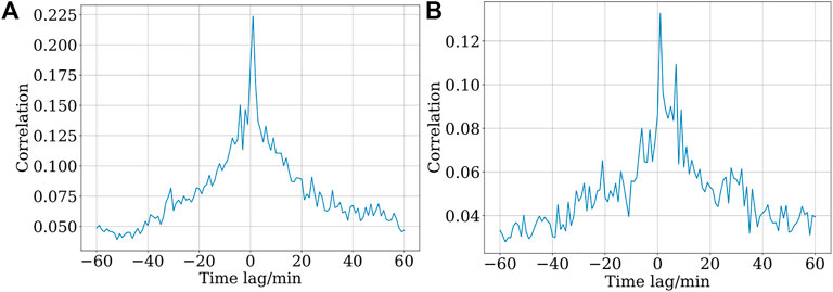
FIGURE 3. (A) Squared volume-weighted price returns–volume correlation. All values of correlation are statistically significant (p-value ≤ 0.001). Permutation significance check indicates no statistically significant correlation between time-permuted squared price returns and volume series. (B) Squared volume-weighted price returns–bid–ask spread correlation. All values of correlation are statistically significant (p-value ≤ 0.001). Permutation significance check indicates no statistically significant correlation between time-permuted squared price returns and volume series.

In Appendix, we plot the same correlation calculation for cryptocurrency-related tweets (see Figure A2A). We do not observe a similar correlation (covariance) pattern as for volume and bid–ask spread signals. Multiple reasons could be behind this: 1) a large noise in the Twitter signal might be covering the information flow w.r.t. trading volume signal, 2) linear dependence might not be enough to capture the relationship, or 3) Twitter signal might not contain a sufficient information flow to influence price volatility. If noise is i.i.d., then “integrated external signal” $\tilde{I}\left(t\right)={\displaystyle {\int }_{t-\delta }^t{I}_{t}dt}$ should filter the noise component. We observe that the stronger correlation pattern is present after the Twitter series is integrated with δ = 30 min (see Appendix Figure A2B), which indicates that strong noise is present in Twitter series.

4 Transfer Entropy Between Information Flow and Volatility Proxy

To proceed, we move from the linear dependence that is captured with correlation $\rho \left(r_t^2,v_t\right)$ to check the nonlinear dependence argument between the squared returns and external information flow $I_t$ signals (volume, bid–ask spread, and Twitter) in causal setting $r_t^2=f\left(I_{t-1},r_{t-1}\right)$. In particular, for the squared price return process $\left\{r_t^2\right\}$ and external information proxy process $\left\{I_t\right\}$, we calculate transfer entropy (TE) [38].

$T{E}_{I\to r^2}:=H\left(r_{t+1}^2|r_t^2\right)-H\left(r_{t+1}^2|r_t^2,I_t\right),(6)$

where $H\left(X|Y\right):=-{\displaystyle {\sum }_{i,j}p\left(x_i,y_j\right)\text{log}\left[p\left(x_i|y_j\right)\right]}$ denotes the conditional Shannon entropy. Transfer entropy is an information-theoretic measure that is both nonlinear and nonsymmetric, and it does not require a Gaussian assumption for the time series [39]. The nonsymmetry allows us to distinguish the direction of information exchange between time series, $I_t$ and $r_t^2$. In Figure 4, we present the results for transfer entropy from external variables to squared returns time series and conversely. The stationarity of the series was checked using the ADF test and the hypothesis of the unit root was rejected at a 1% significance. Results of the transfer entropy analysis show that values are significant, with the largest one being the transfer entropy from squared returns to trading volume. The statistical significance (p-value) of transfer entropy was estimated by a bootstrap method of the underlying Markov process [40]. To account for the finite sample size, we use the effective transfer entropy (ETE) measure:

$ET{E}_{I\to r^2}=T_{I\to r^2}-\frac{1}{M}{\displaystyle \sum _{m=1}^M{T}_{I_{\left(m\right)}\to r^2}},(7)$

where $I_{\left(m\right)}$ is the mth shuffled series of I [41]. We observe a stronger information transfer from the volume signal and the bid–ask spread to squared returns than from the Twitter signal to squared returns. At this point, we conclude that all external signals show significant dependence toward the proxy for volatility signal, that is, squared returns.

FIGURE 4

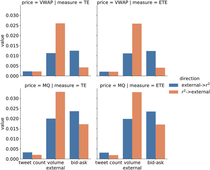
FIGURE 4. Transfer entropy (TE) and effective transfer entropy (ETE) between external signals (Twitter, volume, and bid–ask spread) and squared returns (VWAP and mid-quote price returns). All transfer entropy results are statistically significant (p-value smaller than 0.001), additionally the presence of unit-roots was checked with augmented Dickey–Fuller test ($\alpha =0.01$).

5 Generalized Autoregressive Conditional Heteroscedasticity With External Information Flow

Using the transfer entropy analysis, we have found statistically significant dependence between historical information proxy and volatility proxy, but not the actual functional dependence. Therefore, we now turn to the class of generalized autoregressive conditional heteroscedasticity models [6] that will describe the price return process and augment it with the external information flow proxy signal.

The GARCH(1,1) model conditions the volatility on its previous value and the previous value of price returns:

$r_t={\mu }_t+{\epsilon }_t,{\epsilon }_t={\sigma }_t{z}_t,z_t\in N\left(\mathrm{0,1}\right).(8)$

${\sigma }_t^2=\omega +\alpha {\epsilon }_{t-1}^2+\beta {\sigma }_{t-1}^2.(9)$

Large α coefficient indicates that the volatility reacts intensely to market movements, while large β shows that the impact of large volatilities slowly dies out. The volatilities defined by the model display volatility clustering and the respective distribution of price returns are leptokurtic, which agrees with the observations in the real data.

Motivated by MDH and TE analysis, we formed a GARCHX model by adding the proxy for the information flow $I_{t-1}$ directly to the GARCH volatility equation:

${\sigma }_t^2=\omega +\alpha {\epsilon }_{t-1}^2+\beta {\sigma }_{t-1}^2+\gamma I_{t-1}.(10)$

We will compare price volatility predictions of GARCH(1,1) with those of GARCHX (1, 1) to explore how information is absorbed into the emerging cryptocurrency market of Bitcoin.

5.1 Volatility GARCHX Process analysis

We turn our attention to the statistical quantification of the GARCH volatility processes. For fitting the data to a GARCH process and making out-of-sample estimates, we use the rugarch library [42] in R, available from CRAN (https://cran.r-project.org/). Apart from expanding GARCH(1,1) to GARCHX(1,1), we add the exogenous variable to models eGARCH(1,1), cGARCH(1,1), and TGARCH(1,1) as well, to check for improvement in volatility predictions. The conditional variance equations corresponding to these models (see Table 1) are extensions of Eq. 5. eGARCH [43] and TGARCH [44] capture the asymmetry between positive and negative shocks, giving a greater weight to the later ones, with the difference between them being the multiplicative and the additive contribution of historical values, and cGARCH [45] separates long- and short-run volatility components.

TABLE 1

TABLE 1. GARCH family.

To get the intuition on how good the GARCH volatility models are at explaining the volatility, we regress $a\cdot {\sigma }_t^2+b$ on squared returns $r_t^2$ [46], where ${\sigma }_t^2$ is the squared GARCH volatility estimate (out-of-sample). Then, we measure the coefficient of determination $R^2,$ that is, the proportion of the variance in the dependent variable that is predictable from the independent variable. We determine the statistical significance of with the F-test. Additionally, we measure the Pearson correlation coefficient (PCC) of estimated ${\sigma }_t^2$ and squared returns $r_t^2$, along with its statistical significance, Figure 5.

FIGURE 5

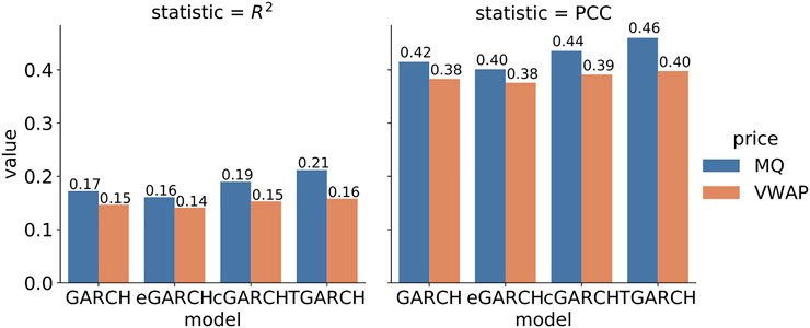
FIGURE 5. Out-of-sample measures for the GARCH volatility process. In-sample consists of 50,000 points and out-of-sample consists of 8000 points. All PCC values are statistically significant. R² statistical significance was checked using F-statistic, and satisfied for all the values.

However, for a more precise statistical quantification of the difference between models and their GARCHX variants, more advanced statistical tests are needed. For that purpose, we employ predictive negative log-likelihood (NLLH) [47].

$\widetilde{\mathrm{ℒ}}=-\text{ln}\left(\mathrm{ℒ}\left({\mu }_1,\dots ,{\mu }_n,{\sigma }_1,\dots ,{\sigma }_n\right)\right)=-{\displaystyle \sum _{i=1}^n\left(\frac{1}{2}\text{ln}\left({\sigma }_i\right)+\frac{1}{2}\text{ln}\left(2\pi \right)-\frac{{\left(r_i-{\mu }_i\right)}^2}{2{\sigma }_i^2}\right)}.(11)$

We evaluated predictive negative log-likelihood (NLLH) on the out-of-sample period. Values of ${\left\{{\mu }_i\right\}}_{i=1}^n$ and ${\left\{{\sigma }_i\right\}}_{i=1}^n$ are predictions of the model, and ${\left\{r_i\right\}}_{i=1}^n$ is the observed price returns. To show whether the improvements can be considered significant, we employed the likelihood ratio test. It takes the natural logarithm of the ratio of two log-likelihoods as the statistic:

$LR=-2\text{ln}\left(\frac{\mathrm{ℒ}\left({\theta }_0\right)}{\mathrm{ℒ}\left(\theta \right)}\right).(12)$

Since its asymptotic distribution is ${\chi }^2$-distribution, a p-value is obtained using Pearson’s chi-squared test. In Figure 6, we see from the p-values that the exogenous variables improve the NLLH significantly for all the models except for eGARCH, for logarithmic returns are created from VWAP. When mid-quote prices are used, a significant improvement is observed only for GARCH and cGARCH.

FIGURE 6

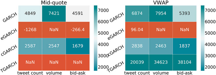
FIGURE 6. Results of out-of-sample likelihood ratio test. In-sample consists of 50,000 points and out-of-sample consists of 8,000 points. *Blue palette represents the p-value smaller than 0.001. NaN—some algorithms had convergence problems.

Note, that for two models with fixed parameters, the likelihood ratio test is the most powerful test at given significance level α, by Neyman–Pearson lemma.

In order to further test the robustness of the conclusions on different samples, we perform the bootstrapping. We restrict the lengths of in-sample and out-of-sample to T = 1000 points each and sample N = 100 such blocks with replacement from the original time series. Then, for each block, we fit a model on its in-sample data segment and calculate predictive out-of-sample NLLH ${\left\{{\widetilde{\mathrm{ℒ}}}_i\right\}}_{i=1}^N$.

In Eq. 11, $M_i$ represents a model from the GARCH family {GARCH, cGARCH, eGARCH, and TGARCH} and $M_{i,j}$ denotes its corresponding GARCHX extension, where external signal $j\in$ {Volume, Twitter, Bid–ask spread}. Models $M_i$ and $M_{i,j}$ will have empirical distribution functions ${\psi }_{M_i}\left(\widetilde{\mathrm{ℒ}}\right)$ and ${\psi }_{M_{i,j}}\left(\widetilde{\mathrm{ℒ}}\right)$, respectively (see boxplots estimates in Figure 7). We calculate the Kolmogorov–Smirnov (KS) statistics between corresponding empirical predictive out-of-sample NLLH distributions:

$K{S}_{i,j}=\underset{\widetilde{\mathrm{ℒ}}}{\text{sup}}\left|{\psi }_{M_i}\left(\widetilde{\mathrm{ℒ}}\right)-{\psi }_{M_{i,j}}\left(\widetilde{\mathrm{ℒ}}\right)\right|,(13)$

and obtain its statistical significance. In Figures 7, 8, we can see that both GARCH and cGARCH models show significant improvements with all the external variables and both price definitions, under the bootstrapping KS-NLLH robustness check. That is not surprising, as the nonparametric KS test is not very powerful [48]. However, significant differences for the GARCH and cGARCH models allow us to confirm that its predictive power is robust under temporal bootstrapping conditions. Finally, we take the GARCH volatility process as a representative and perform additional bootstrapping KS–NLLH robustness checks on two additional segments (March–April 2019 and November–December 2019) and we see similar results (See Appendix Figure A3).

FIGURE 7

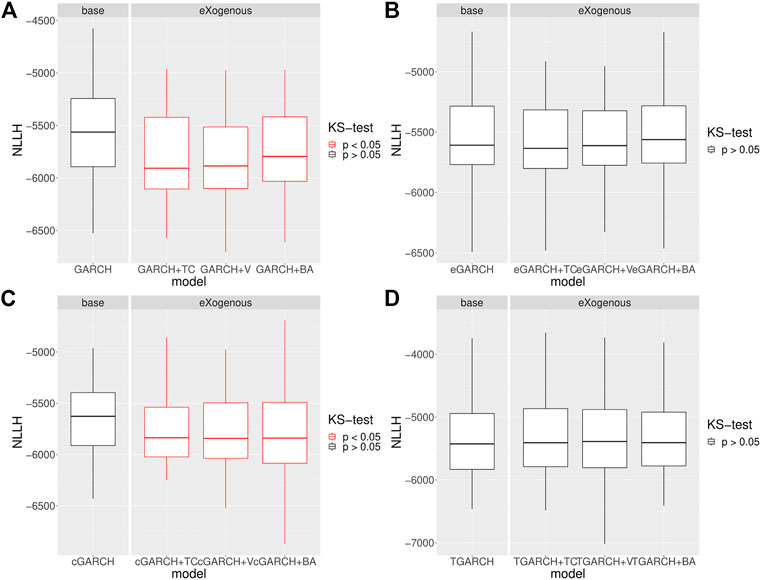
FIGURE 7. Bootstrap robustness check over N = 100 splitting points with T = 1,000 training points and T = 1,000 test size for GARCH and GARCHX models. The price is defined as volume-weighted. The nonparametric Kolmogorov–Smirnov test of the equality of the NLLH out-of-sample distributions between the GARCH and GARCHX models is done. (A) KS test implies a significant difference for both external signals for the GARCH model. (B) KS test implies no significant difference for external signals for the eGARCH model. (C) KS test implies no significant difference for both external signals for the cGARCH model. (D) KS test implies no significant difference for external signals for the TGARCH model.

FIGURE 8

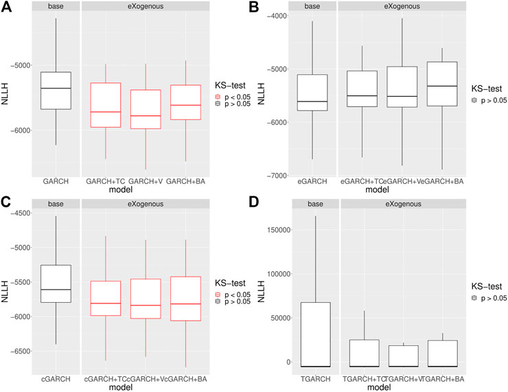
FIGURE 8. Bootstrap robustness check over N = 100 splitting points with T = 1,000 training points and T = 1,000 test size for GARCH and GARCHX models. The price is defined as mid-quote. The nonparametric Kolmogorov–Smirnov test of the equality of the NLLH out-of-sample distributions between the GARCH and GARCHX models is done. (A) KS test implies a significant difference for both external signals for the GARCH model. (B) KS test implies no significant difference for external signals for the eGARCH model. (C) KS test implies no significant difference for both external signals for the cGARCH model. (D) KS test implies no significant difference for external signals for the TGARCH model.

6 Discussion

Although the theoretical foundations of the effects of information on markets have been proposed a long time ago [1, 2], they were further developed in 1970, as “weak”, “semi-strong”, and “strong” forms of efficient market hypothesis [49]. The mathematical models of information effects continued to advance in the 70s as well, by the proposition of the Mixture of Distribution Hypothesis [4], which states that the dynamics of price returns are governed by the information flow available to the traders. Following the growth of computerized systems and the availability of empirical data in the 80s, more elaborate statistical models were proposed, such as generalized autoregressive conditional heteroscedasticity models (GARCH) [6] and news Poisson-jump processes [7] with constant intensity. Furthermore, studies from the 2000s generalized the news Poisson-jump processes by introducing time-varying jump effects, supporting it with the statistical evidence of time variation in the jump size distribution [8, 9].

In this article, we have analyzed the effects of information flow on the cryptocurrency Bitcoin exchange market that appeared with the introduction of blockchain technology in 2008 [11]. Although the trading volume in the largest cryptocurrency markets has grown exponentially in the last 10 years, still the research on their (in)efficiency quantification is ongoing [50, 51]. We have focused on the Bitcoin, the largest cryptocurrency w.r.t. market capitalization, and used the reliable data of price returns and traded volume and bid–ask spread from Bitfinex exchange market [52] on a minute-level granularity. The price returns were calculated using two different definitions, VWAP and mid-quote, to account for possible market-microstructure noise. Another reason, why we have concentrated on the Bitcoin, was the availability of Twitter-related data [36]. We have used the social media signals from Twitter, trading volume and bid–ask spread from the Bitcoin market as a proxy for information flow together with the GARCH family of [53] processes to quantify the prediction power for the price volatility.

We started the analysis by employing recently developed nonparametric information-theoretic transfer entropy measures [38, 40, 41], to confirm the nonlinear relationship between the exogenous proxy for information (trading volume, bid–ask spread, and cryptocurrency related tweets) and squared price returns (proxy for volatility). Further on, we have made extensive experiments on the following models: GARCH, eGARCH, cGARCH, and TGARCH on the minute-level data of price returns, Twitter volume, exchange volume data, and bid–ask spread. Our testing procedure consisted of multi-stage statistical checks: 1) out-of-sample $R^2$ and Pearson correlation measurements, 2) out-of-sample predictive likelihood measurements with the likelihood ratio test on 8,000 points, and 3) bootstrapped predictive likelihood measurements with the nonparametric Kolmogorov–Smirnov test. From the predictive perspective of the nonlinear parametric GARCH model, we have found that exogenous proxy for information flow significantly improves out-of-sample minute volatility predictions for the GARCH and cGARCH [54] models. It is not surprising that the basic GARCH model is outperforming more advanced models [46, 55] such as eGARCH [43] and TGARCH [44] on out-of-sample data. Also, a previous study [18] found that the cGARCH model on the Bitcoin market was performing the best on in-sample daily returns.

Finally, we have taken the GARCH model and applied the bootstrapping on two additional segments (March–April 2019 with 38,000 points and November–December 2019 with 52,000 points) and we observe that our observations still hold (see Appendix Figure A3). For future work, we leave focusing on other cryptocurrencies and analyzing the cross-market volatility spillovers, in which different market behavior modes could be studied separately.

Data Availability Statement

For accessing the data please contact the corresponding author at anino@ethz.ch.

Author Contributions

IB performed experiments, NA-F supervised the research, and both authors analyzed the results and wrote the manuscript.

Funding

NA-F acknowledges financial support from SoBigData++ through Grant Agreement No. 871042. IB acknowledges the SoBigData TransNational Access research visit and partial support form QuantiXLie Centre of Excellence, a project co-financed by the Croatian Government and European Union through the European Regional Development Fund-the Competitiveness and Cohesion Operational Program (Grant KK.01.1.1.01.0004, elementleader N.P.).

Conflict of Interest

The authors declare that the research was conducted in the absence of any commercial or financial relationships that could be construed as a potential conflict of interest.

Acknowledgments

We would like to thank Tian Guo and Fabrizio Lillo for helpful discussions.

Appendix

FIGURE A1

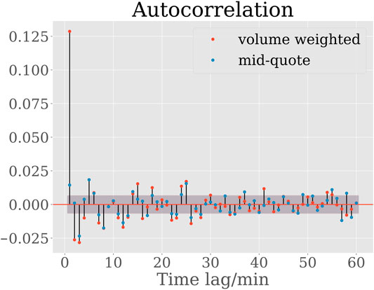
FIGURE A1. Autocorrelation of price returns. The first-order autocorrelation of mid-quote price returns is significantly smaller than that of volume-weighted price returns, indicating a smaller level of microstructure noise in mid-quote price returns. Confidence interval.

FIGURE A2

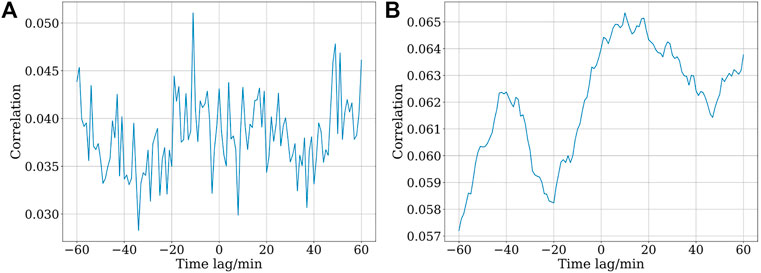
FIGURE A2. (A) Correlation between squared price returns and Twitter volume. Permutation significance check indicates no statistically significant correlation between time-permuted squared price returns and Twitter time series. (B) Correlation between squared price returns and integrated Twitter volume (over a 30-min moving window). This test is only used to check whether the integrating operator is filtering noise. Correlation between squared price returns and Twitter time series. All values of correlation are statistically significant (p-value $\le 0.001$).

FIGURE A3

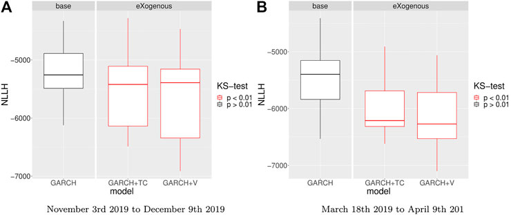
FIGURE A3. Bootstrap robustness check over N = 100 splitting points with T = 1000 training points and T = 1000 points in test size for GARCH and GARCHX models. The nonparametric Kolmogorov–Smirnov test of the equality of the NLLH out-of-sample distributions between GARCH and GARCHX models is done. (A) KS test implies a significant difference for all external signals for the GARCH model in the period from November 3rd, 2019 to December 9th, 2019 with 52,000 observations. (B) KS test implies a significant difference for all external signals for the GARCH model in the period from March 18th, 2019, to April 9th, 2019, with 38,000 observations.

References

1. Bachelier L. Louis Bachelier’s Theory of Speculation: The Origins of Modern Finance. New Jersey: Princeton University Press (2011). doi:10.1515/9781400829309

CrossRef Full Text

2. Mandelbrot B. The Variation of Certain Speculative Prices. J Bus (1963) 36(4):394–419. doi:10.1086/294632

CrossRef Full Text | Google Scholar

3. Stanley H, Mantegna R. An Introduction to Econophysics. Cambridge: Cambridge University Press (2000).

4. Clark PK. A Subordinated Stochastic Process Model with Finite Variance for Speculative Prices. Econometrica (1973) 41(1):135. doi:10.2307/1913889

CrossRef Full Text | Google Scholar

5. Engle RF. Autoregressive Conditional Heteroscedasticity with Estimates of the Variance of United Kingdom Inflation. Econometrica (1982) 50:987–1007. doi:10.2307/1912773

CrossRef Full Text | Google Scholar

6. Bollerslev T. Generalized Autoregressive Conditional Heteroskedasticity. J Econom (1986) 31(3):307–27. doi:10.1016/0304-4076(86)90063-1

CrossRef Full Text | Google Scholar

7. Jorion P. On Jump Processes in the Foreign Exchange and Stock Markets. Rev Financ Stud (1988) 1(4):427–45. doi:10.1093/rfs/1.4.427

CrossRef Full Text | Google Scholar

8. Chan WH, Maheu JM. Conditional Jump Dynamics in Stock Market Returns. J Business Econ Stat (2002) 20(3):377–89. doi:10.1198/073500102288618513

CrossRef Full Text | Google Scholar

9. Maheu JM, McCurdy TH. News Arrival, Jump Dynamics, and Volatility Components for Individual Stock Returns. J Finance (2004) 59(2):755–93. doi:10.1111/j.1540-6261.2004.00648.x

CrossRef Full Text | Google Scholar

10. Chuen D. Handbook of Digital Currency: Bitcoin, Innovation, Financial Instruments, and Big Data. Amsterdam: Academic Press (2015). doi:10.1016/C2014-0-01905-3

CrossRef Full Text

11. Nakamoto S. Bitcoin: A Peer-To-Peer Electronic Cash System (2008). https://bitcoin.org/bitcoin.pdf

12. Gandal N, Hamrick J, Moore T, Oberman T. Price Manipulation in the Bitcoin Ecosystem (2017). CEPR Discussion Papers 12061.

Google Scholar

13. Ciaian P, Rajcaniova M, Kancs d. A. The Economics of Bitcoin Price Formation. Appl Econ (2016) 48:1799–815. doi:10.1080/00036846.2015.1109038

CrossRef Full Text | Google Scholar

14. Cheah E-T, Fry J. Speculative Bubbles in Bitcoin Markets? an Empirical Investigation into the Fundamental Value of Bitcoin. Econ Lett (2015) 130:32–6. doi:10.1016/j.econlet.2015.02.029

CrossRef Full Text | Google Scholar

15. Kristoufek La. What Are the Main Drivers of the Bitcoin Price? Evidence from Wavelet Coherence Analysis. PloS one (2015) 10(4):e0123923. doi:10.1371/journal.pone.0123923

PubMed Abstract | CrossRef Full Text | Google Scholar

16. Donier J, Bouchaud J-P. Why Do Markets Crash? Bitcoin Data Offers Unprecedented Insights. PLOS ONE (2015) 10:1–11. doi:10.1371/journal.pone.0139356

PubMed Abstract | CrossRef Full Text | Google Scholar

17. Wheatley S, Sornette D, Huber T, Reppen M, Gantner RN. Are Bitcoin Bubbles Predictable? Combining a Generalized Metcalfe’s Law and the Lppls Model (March 15, 2018). Swiss Finance Institute Research Paper Available at SSRN: https://ssrn.com/abstract=3141050 or http://dx.doi.org/10.2139/ssrn.3141050.

CrossRef Full Text

18. Katsiampa P. Volatility Estimation for Bitcoin: A Comparison of GARCH Models. Econ Lett (2017) 158:3–6. doi:10.1016/j.econlet.2017.06.023

CrossRef Full Text | Google Scholar

19. Guo T, Bifet A, Antulov-Fantulin N. “Bitcoin Volatility Forecasting with a Glimpse into Buy and Sell Orders,” in 2018. IEEE Int Conf Data Mining (Icdm) Nov (2018) 989–94. doi:10.1109/ICDM.2018.00123

CrossRef Full Text | Google Scholar

20. Ron D, Shamir A. Quantitative Analysis of the Full Bitcoin Transaction Graph. In: International Conference On Financial Cryptography And Data Security. Springer (2013). p. 6–24. doi:10.1007/978-3-642-39884-1_2

CrossRef Full Text | Google Scholar

21. ElBahrawy A, Alessandretti L, Kandler A, Pastor-Satorras R, Baronchelli A. Evolutionary Dynamics of the Cryptocurrency Market, R. Soc. Open Sci. R Soc Open Sci (2017) 4(11):170623. doi:10.1098/rsos.170623

PubMed Abstract | CrossRef Full Text | Google Scholar

22. Antulov-Fantulin N, Tolic D, Piskorec M, Ce Z, Vodenska I. Inferring Short-Term Volatility Indicators from the Bitcoin Blockchain. In: Complex Networks And Their Applications VII. Cham: Springer International Publishing (2019). p. 508–20. doi:10.1007/978-3-030-05414-4_41

CrossRef Full Text | Google Scholar

23. Hayes A, “Cryptocurrency Value Formation: An Empirical Analysis Leading to a Cost of Production Model for Valuing Bitcoin.”(2015). Telematics and Informatics, Forthcoming, Available at SSRN: https://ssrn.com/abstract=2648366,

Google Scholar

24. Bolt W. On the Value of Virtual Currencies. De Nederlandsche Bank Working Paper No. 521 (2016). Available at SSRN: https://ssrn.com/abstract=2842557.

Google Scholar

25. Nadarajah S, Chu J. On the Inefficiency of Bitcoin. Econ Lett (2017) 150:6–9. doi:10.1016/j.econlet.2016.10.033

CrossRef Full Text | Google Scholar

26. Kristoufek L. Bitcoin Meets Google Trends and Wikipedia: Quantifying the Relationship between Phenomena of the Internet Era. Scientific Rep (2013) 3:3415. doi:10.1038/srep03415

PubMed Abstract | CrossRef Full Text | Google Scholar

27. Li TR, Chamrajnagar AS, Fong XR, Rizik NR, Fu F. Sentiment-based Prediction of Alternative Cryptocurrency Price Fluctuations Using Gradient Boosting Tree Model (2018). Papers 1805.00558, arXiv.org.

Google Scholar

28. Kim YB, Kim JG, Kim W, Im JH, Kim TH, Kang SJ, et al. Predicting Fluctuations in Cryptocurrency Transactions Based on User Comments and Replies. PloS one (2016) 11. doi:10.1371/journal.pone.0161197

PubMed Abstract | CrossRef Full Text | Google Scholar

29. Garcia D, Schweitzer F. Social Signals and Algorithmic Trading of Bitcoin. R Soc Open Sci (2015) 2(9):150288. doi:10.1098/rsos.150288

PubMed Abstract | CrossRef Full Text | Google Scholar

30. Dey AK, Akcora CG, Gel YR, Kantarcioglu M. On the Role of Local Blockchain Network Features in Cryptocurrency Price Formation. Can J Stat (2020) 48(3):561–81. [Online]. Available: https://onlinelibrary.wiley.com/doi/abs/10.1002/cjs.11547. doi:10.1002/cjs.11547

CrossRef Full Text | Google Scholar

31. Naimy V, Haddad O, Fernández-Avilés G, El Khoury R. The Predictive Capacity of Garch-type Models in Measuring the Volatility of Crypto and World Currencies. PLOS ONE (2021) 16(1):e0245904–17. doi:10.1371/journal.pone.0245904

PubMed Abstract | CrossRef Full Text | Google Scholar

32. Chu J, Chan S, Nadarajah S, Osterrieder J. Garch Modelling of Cryptocurrencies. J Risk Financial Manag (2017) 10(4). [Online]. Available: https://www.mdpi.com/1911-8074/10/4/17. doi:10.3390/jrfm10040017

CrossRef Full Text | Google Scholar

33. Shen D, Urquhart A, Wang P. Does Twitter Predict Bitcoin? Econ Lett (2019) 174:118–22. [Online]. Available: https://www.sciencedirect.com/science/article/pii/S0165176518304634. doi:10.1016/j.econlet.2018.11.007

CrossRef Full Text | Google Scholar

34. Gao X, Huang W, Wang H. Financial Twitter Sentiment on Bitcoin Return and High-Frequency Volatility. Virtual Econ (2021) 4(1):7–18. Jan. [Online]. Available: https://www.virtual-economics.eu/index.php/VE/article/view/101. doi:10.34021/ve.2021.04.01(1)

CrossRef Full Text | Google Scholar

35. Gatheral J, Oomen RCA. Zero-intelligence Realized Variance Estimation. Finance Stoch (2010) 14(2):249–83. [Online]. Available: https://ideas.repec.org/a/spr/finsto/v14y2010i2p249-283.html. doi:10.1007/s00780-009-0120-1

CrossRef Full Text | Google Scholar

36. Beck J, Huang R, Lindner D, Guo T, Ce Z, Helbing D, et al. Sensing Social Media Signals for Cryptocurrency News. In: Companion Proceedings Of the 2019 World Wide Web Conference (2019). p. 1051–4.

Google Scholar

37. Tauchen GE, Pitts M. The Price Variability-Volume Relationship on Speculative Markets. Econometrica (1983) 51(2):485–505. doi:10.2307/1912002

CrossRef Full Text | Google Scholar

38. Schreiber T. Measuring Information Transfer. Phys Rev Lett (2000) 85(2):461–4. doi:10.1103/physrevlett.85.461

PubMed Abstract | CrossRef Full Text | Google Scholar

39. Barnett L, Barrett AB, Seth AK. Granger Causality and Transfer Entropy Are Equivalent for Gaussian Variables. Phys Rev Lett (2009) 103(23). doi:10.1103/PhysRevLett.103.238701

PubMed Abstract | CrossRef Full Text | Google Scholar

40. Dimpfl T, Peter FJ. Using Transfer Entropy to Measure Information Flows between Financial Markets. Stud Nonlinear Dyn Econom (2013) 17(1):85–102. doi:10.1515/snde-2012-0044

CrossRef Full Text | Google Scholar

41. Marschinski R, Kantz H. Analysing the Information Flow between Financial Time Series. Eur Phys J B (2002) 30(2):275–81. doi:10.1140/epjb/e2002-00379-2

CrossRef Full Text | Google Scholar

42. Ghalanos A, Rugarch: Univariate GARCH Models.,(2020), r package version 1.4-4.

Google Scholar

43. Nelson DB. Conditional Heteroskedasticity in Asset Returns: A New Approach. Econometrica (1991) 59(2):347–70. doi:10.2307/2938260

CrossRef Full Text | Google Scholar

44. Zakoian J-M. Threshold Heteroskedastic Models. J Econ Dyn Control (1994) 18(5):931–55. doi:10.1016/0165-1889(94)90039-6

CrossRef Full Text | Google Scholar

45. Lee G, Engle R. A Permanent and Transitory Component Model of Stock Return Volatility. In: WJ Granger Cointegration, Causality And Forecasting: A Festschrift In Honor Of Clive (1999). p. 475–97.

Google Scholar

46. Andersen TG, Bollerslev T. Answering the Skeptics: Yes, Standard Volatility Models Do Provide Accurate Forecasts. Int Econ Rev (1998) 39:885–905. doi:10.2307/2527343

CrossRef Full Text | Google Scholar

47. Wu Y, Hernández-Lobato JM, Ghahramani Z. Gaussian Process Volatility Model. In: NIPS (2014). p. 1044–52.

Google Scholar

48. Marozzi M. Nonparametric Simultaneous Tests for Location and Scale Testing: A Comparison of Several Methods. Commun Stat - Simulation Comput (2013) 42(6):1298–317. doi:10.1080/03610918.2012.665546

CrossRef Full Text | Google Scholar

49. Fama EF. Efficient Capital Markets: A Review of Theory and Empirical Work. J Finance (1970) 25(2):383. doi:10.2307/2325486

CrossRef Full Text | Google Scholar

50. Tran VL, Leirvik T. Efficiency in the Markets of Crypto-Currencies, Finance Res Lett, 35 (2019). p. 101382. doi:10.1016/j.frl.2019.101382

CrossRef Full Text | Google Scholar

51. Kristoufek L, Vosvrda M. Cryptocurrencies Market Efficiency Ranking: Not So Straightforward. Physica A: Stat Mech its Appl (2019) 531:120853. doi:10.1016/j.physa.2019.04.089

CrossRef Full Text | Google Scholar

52. Hougan M, Kim H, Lerner M, Management BA. “Economic and Non-economic Trading in Bitcoin: Exploring the Real Spot Market for the World’s First Digital Commodity. Bitwise Asset Management (2019). https://www.sec.gov/comments/sr-nysearca-2019-01/srnysearca201901-5574233-185408.pdf

53. Engle R. New Frontiers for Arch Models. J Appl Econ (2002) 17(5):425–46. doi:10.1002/jae.683

CrossRef Full Text | Google Scholar

54. Engle RF, Sokalska ME. Forecasting Intraday Volatility in the Us Equity Market. Multiplicative Component Garch. J Financial Econom (2012) 10(1):54–83. doi:10.1093/jjfinec/nbr005

CrossRef Full Text | Google Scholar

55. Jafari GR, Bahraminasab A, Norouzzadeh P. Why Does the Standard Garch(1, 1) Model Work Well? Int J Mod Phys C (2007) 18(07):1223–30. doi:10.1142/s0129183107011261

CrossRef Full Text | Google Scholar