 Yingqing Huang1
 Xingpeng Yan
- 1Department of Weapons and Control, Army Academy of Armored Forces, Beijing, China
- 2Department of Information Communication, Army Academy of Armored Forces, Beijing, China
- 3Department of Basic Education, Army Academy of Armored Forces, Beijing, China
- 4Jiangsu North Huguang Opto-Electronics Co., LTD, Wuxi, China
Integral imaging is an emerging three-dimensional display technology. However, some inherent issues such as depth inversion has restricted its development. As such, this paper proposes a pixel fusion technique to generate elemental image arrays and overcome pseudoscopic problems occurring in sparse imaging environments. The similarity between the aimed displayed rays and the two adjacent captured rays of an object in a parallel light field was measured by the ratio of the spatial distance of the displayed and captured rays to the interval of the adjacent captured light. Displayed pixel values were acquired for the parallel captured rays. Corresponding pixel position errors were determined in sparse capture conditions and the method was further improved by using the position errors to identify the correct pixel, resulting in higher image quality. The proposed technique does not require manual adjustment of reference planes or other parameters, even at low capturing densities. This provides added convenience and may reduce capturing costs in actual scenes. Experiments using two bricks in virtual scenes under 9 × 9 to 137 × 137 capture cameras were conducted, and the quality of the generated elemental image array was compared with smart pseudoscopic-to-orthoscopic conversion (SPOC). The peak signal-to-noize ratio (PSNR) and structural similarity (SSIM) values showed the effectiveness of the proposed technique. The optical reconstruction results from both real and virtual scenes demonstrated improvements in vision of reconstructed three-dimensional scenes.
Introduction
Since its initial development, integral imaging (InIm) has generated significant interest for use in light field displays, because of its ability to represent three-dimensional (3D) images with full-color parallax [1]. The ideal 3D light field can accurately reconstruct depth information for a recorded object and display a realistic suspended object. The acquisition of light field data can generally be divided into physical acquisition and computer rendering steps. When using captured pictures to generate the elemental image array (EIA), it is necessary to compensate for inconsistencies in acquisition camera and display lens parameters. The resolution of acquired pictures can also affect the elemental image (EI) and the depth inversion (or the pseudoscopic properties [2]) of the displayed images. Among these issues, pseudoscopic characteristics have the most direct influence. The inversion of depth information can also cause reconstructed 3D scenes to appear unrealistic to an observer.
Multiple studies have attempted to overcome the pseudoscopic nature of displayed images. For example, Okano et al. [3] used a television camera in the capturing stage and rotated each captured image by 180° around the center of the elemental cell. This approach is simple and offers fast speed. However, it requires acquisition and display lens parameters to be similar to each other. In addition, reconstructed 3D scenes are virtual, which prevents the technique from being applied universally. Martínez-Corral and Javidi et al. proposed smart pixel mapping (SPM) [4], later improving on the technique [5]. These algorithms can produce 3D images exhibiting an out-of-screen effect, without the limitations of capture or display system parameters. This group later proposed a more widely applicable smart pseudoscopic-to-orthoscopic conversion (SPOC) model [6], which provided orthoscopic 3D scenes and overcame parameter mismatch problems between the capture and display systems. However, the technique requires a virtual reference plane and errors in plane selection can seriously affect the final EIA quality. Other groups have improved this technique by establishing multiple pre-selected reference planes [7]. The resulting EIA quality improved as a result, however, the 3D scenes needed to be segmented into several subregions. The size of these subregions could be optimized empirically. Deng et al. [8] conducted research on sparse acquisition and proposed a methodology for generating orthoscopic EIA by mapping all pixels in a parallax image array to the focal plane of the micro-lenses. Other groups [9, 10] have improved this technique by investigating the differences between multi-view display (MVD) and InIm systems. An improved methodology was also proposed which, due to the periodic appearance of depth planes, permitted adjustable depth positions in displayed 3D scenes. However, the display device could only be placed at the periodic depth plane. In addition, due to the needed precision, the technique also requires a special number of capture cameras. Piao et al. [11] proposed a methodology that permits the display of orthoscopic 3D scenes at arbitrary positions, by processing captured picture data based on the coverage of a display lens. Recently, Zhu et al. [12] used piecewise tracking to overcome pseudoscopic limitations while simultaneously enlarging the field of view. Wang et al. [13] analyzed mismatches between acquisition and display systems, performing a pixel remapping on the acquired pictures after they were cut and expanded. Liu et al. [14] proposed a light field resampling method for generating EIA to break through the constraints between the record device and display device. Zhang et al. [15] proposed an optical method to eliminate the pseudoscopic issue using a transmissive mirror device (TMD) and a light filter to eliminate the ghost images caused by the TMD. In addition, our group [16] has proposed a lens array shifting technique to improve display performance by achieving higher quality EIA, however, the complex synchronization issues and mechanical vibration limit the conditions of use.
The high-quality 3D reconstruction of real scenes is one of the primary goals for InIm. In addition to overcoming pseudoscopic and parameter matching problems, the capture system in real scenes is also limited by cost and implementation complexities such as the capture space, system structure and data transmission. As a result, capture camera density is typically sparse. Therefore, it is of practical value to study high-quality EIA generation methods in sparse acquisition conditions.
In this study, a new EIA generation technique is proposed to overcome pseudoscopic problems in sparse captured pictures. The relationship between adjacent parallel captured rays and displayed rays is analyzed by spatial position, suggesting captured rays can be used to estimate displayed rays. In sparse capturing, potential areas in adjacent captured pictures are matched to determine the most likely displayed ray. By measuring the distance between adjacent displayed rays and captured rays, pixels in captured images can be fused and used to calculate the required EIA. However, the proposed methodology does not require the selection of reference planes. There are also no requirements for the captured system or display parameters when operating at low capturing densities. This allows for simple adaptation to different display systems and can reduce capturing costs in real scenes. In the following sections, the underlying principles governing this proposed technique are explained in detail and a series of validation experiments are conducted to verify its effectiveness.
Light Field Analysis
Light emitted by the display system must have the same intensity in the same direction as light recorded by the capture system, to ensure the scene displays correctly. The observer and capture systems are typically on the same side of the object, such that captured pictures can be directly used for display. Although the intensity of the light remains constant, the direction varies widely, leading to pseudoscopic issues. As shown in Figure 1, the cube is positioned in front of the cylinder when it is captured, while the cylinder is in front of the cube when displayed from the viewing direction. Pseudoscopic problems are primarily caused by differences in the direction of the light field during object capture and display. This configuration can be made more intuitive by assuming the display system and capture system (observer) are located on both sides of the object and that light emitted by the display system is recorded by the capture system. In this way, the correctness of the generated image depth can be ensured.
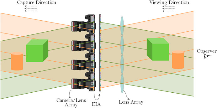
FIGURE 1. Pseudoscopic issues in integral imaging.
Characteristics of the Light Field
As shown in Figure 2, the camera is equivalent to a lens model. Since the parameters for each acquisition unit are the same in the capture system, light rays corresponding to pixels at the same positions in different units are parallel to each other. This corresponds to a set of object components in a specific direction. The magnitude of these pixels represents the intensity for different object components in each direction, as indicated by the solid line in the figure. In real space, light intensity from an object varies continuously in a given direction. After passing through the capture system, the continuously changing light intensity is sampled and quantified. The corresponding sampling space interval is thus equivalent to the distance of the center of the adjacent lenses. Light intensity information is then recorded on a storage medium such as a CCD. Similarly, in the display system, pixels at the same position under different lenses also constitute parallel light in space. When the direction of the light matches that of the capture system, this forms a set of parallel light field components. When displayed correctly, light from the parallel field components mimics the captured light. Ideally, as the light passes through the optical center of the lens, in both the capture and display systems, light emitted by the display system completely overlaps light recorded by the capture system. Thus, these two signals have the same physical meaning and exhibit the same pixel values. However, in reality, the displayed and captured rays do not coincide exactly and pixels cannot be directly assigned.
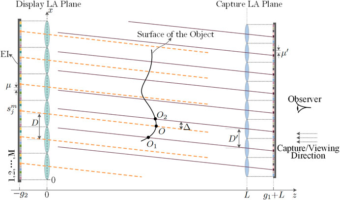
FIGURE 2. The relationship between capture and display rays.
A coordinate system can be established for any angular component in a parallel light field, as shown in Figure 2. In this configuration, the bottom end in the vertical direction of the display lens serves as the coordinate origin, the distance between the plane of the display lens array and the capture lens array is represented by L and the distance between the plane of the capture lens array and the captured image array is given by g1. On the capturing end, the distance between the adjacent capturing lenses is denoted by Dʹ and the distance between adjacent pixels in the captured image is represented by
and the number of the corresponding capture lenses is denoted as:
where
The next nearest capture lens is represented by:
In the captured image, the index of pixels corresponding to the captured light (parallel to the display light) is given by:
From this analysis, the final pixel value can be expressed as:
where
Analysis of Pixel Positioning Errors
The conclusions described above are based on the tight arrangement of the capture lenses. In the parallel light field, the distance between the display light and the capture light is sufficiently small (at any angle) that deviations in pixel values caused by positioning differences are also small. As a result, any effects on the display are negligible. However, in practical scenarios, dense capture systems consume a significant amount of resources and are limited by cost and difficulty of implementation. As such, the actual capture system lens interval is typically large, leading to errors if Eq. 6 is used directly. This can seriously affect the accuracy of reconstructed light fields.
The intersection of the display light and the surface of the object is denoted by O in Figure 3. The intersection of the adjacent captured light and the surface of the object is represented by O1 and O2, and the distance between the displayed light and the nearest captured light is Δ. The distance between adjacent captured light rays in the same parallel light field is relatively large, due to large distances between the capture lenses. As a result, information such as the color and intensity of adjacent parallel captured light rays exhibits obvious differences and can no longer be considered the same area. Assuming the distance from O to the display lens array is given by l, pixel position errors for O and O1 imaging through lens 1 can be represented as
In Eqs. 7 and 8, the terms
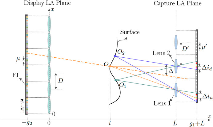
FIGURE 3. Errors in capture and display rays.
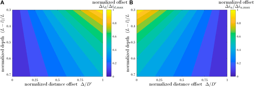
FIGURE 4. Normalized offsets for pixel positions with different system parameters: (A)
As seen in Figures 4A and 4B, pixel position errors are larger when the object depth position is closer to the capture lens array (i.e.,
Pixel Fusion Under Sparse Acquisition Conditions
Equation 9 represents the range of pixels for which the surface area of the object,
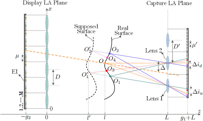
FIGURE 5. Errors in capture and display rays.
From this analysis, the positions of common areas (determined by adjacent rays in the captured picture) can be identified by assuming the positions of the object surface and calculating the similarity of the corresponding captured pixel values. This was done while taking both complexities, accuracy and robustness of the algorithm into account. The sum of squared differences (SSD) model, commonly applied in image processing, was used as the criterion for similarity judgments. At a distance z from the display lens array, the value of SSD corresponding to the mth display pixel is given by:
In this expression,
where
This approach can be summarized as follows shown in Figure 6.
(1) Calculate the intersection coordinates x of the displayed light emitted from the aimed pixel j.
(2) Determine the number of the corresponding nearest neighbor capture lens n and the next-nearest neighbor capture lens n′ by x.
(3) Determine the pixel position i for the corresponding parallel captured light in the images, according to the direction of the displayed light.
(4) calculate the distance Δ between the displayed light and the nearest captured light.
(5) Find the appropriate z that minimizes
(6) determine the aimed pixel errors
(7) Calculate the specific pixel values using Eq. 11.
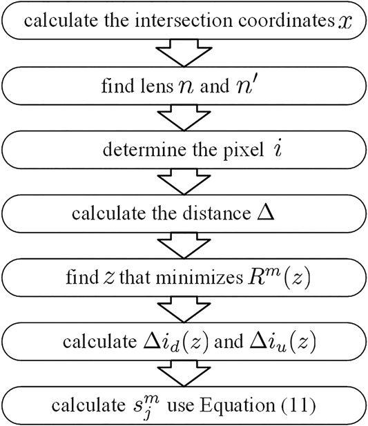
FIGURE 6. Steps of the proposed pixel fusion method.
Experimental Verification
The display system used in the experiment consisted of a lens array, a display device, and a linear track. As shown in Figure 7, unit lenses in the lens array were arranged in a 50 × 50 square grid. The length and width of the unit lenses were each 2 mm and the focal length was 8 mm. An LCD mobile phone screen was used as the display device, offering a resolution of 3,840 × 2,160 and a pixel pitch of 0.0315 mm. During the experiment, the LCD was fixed on a linear track with a step size of 0.01 mm. The positions of the lens array and LCD were adjusted to ensure the best display effects.
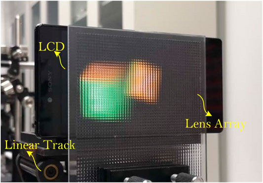
FIGURE 7. The display system used in the experiments.
The Performance of Virtual Scenes
The effectiveness of the proposed technique in displaying virtual scenes was verified using 3Dmax for object capture, as demonstrated in Figure 8A. The FOV for the virtual camera was 14.2°, the resolution was 179 × 179, the size of the camera array was 23 × 23, the grid was square, and the distance between adjacent cameras was 2 mm. Two cubic toy bricks, with side lengths of 20 mm, were used as a model. The geometric center of the left brick was 60 mm from the virtual camera array plane, while the right brick center was 100 mm away. A frontal view of this model is shown in Figure 8B. In the experiment, the distance between the display lens array and the camera array was set to 160 mm. The classic SPOC model was used to provide a comparison and verify the effectiveness of the proposed technique. The EIAs generated by the two methods are shown in Figure 9.
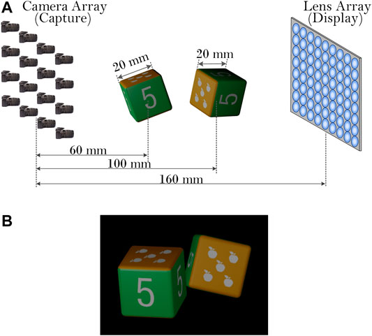
FIGURE 8. (A) Scene settings for the virtual acquisition experiment. (B) The frontal scene view.
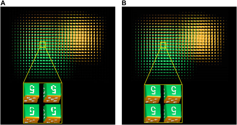
FIGURE 9. (A) The EIA generated by SPOC with the reference plane at 80 mm. (B) The EIA generated by the proposed method.
As the EIAs shown in Figure 9, while they exhibit similar structure, obvious differences are evident in the close-up views. Specifically, significant mosaic effects are present in the SPOC results. There is also a pronounced difference in the number “5” shown in Figure 9A, as the line thickness is uneven and some areas were not displayed normally. The primary reason for this error is that selection of a reference plane is not consistent with the actual object location. The EI generated by the proposed technique can more easily compensate for mosaic artifacts, as shown in Figure 9B. As a result, the number “5” is closer to that of the original scene and maintains better consistency with varying EIs. In addition, all components can be displayed normally and the thickness of the line is more uniform. This suggests the quality of EIA generation is related to the complexity of the scene. When the scene is relatively simple (e.g., the surfaces of a cube), pixel values at different positions do not vary significantly and there is little difference between the EI generated using each algorithm. As the complexity of a scene increases (e.g., adding numbers to the cube), the probability of numerical differences caused by pixel position errors will increase. This in turn will lead to differences in the EI components generated by each method. These results suggest the proposed technique can accurately calculate details in three-dimensional scenes. Display results for each model were compared by loading the generated EIA into a display system. Optical reconstructions were then acquired at a distance of 1 m from the display lens array, as shown in Figure 10.
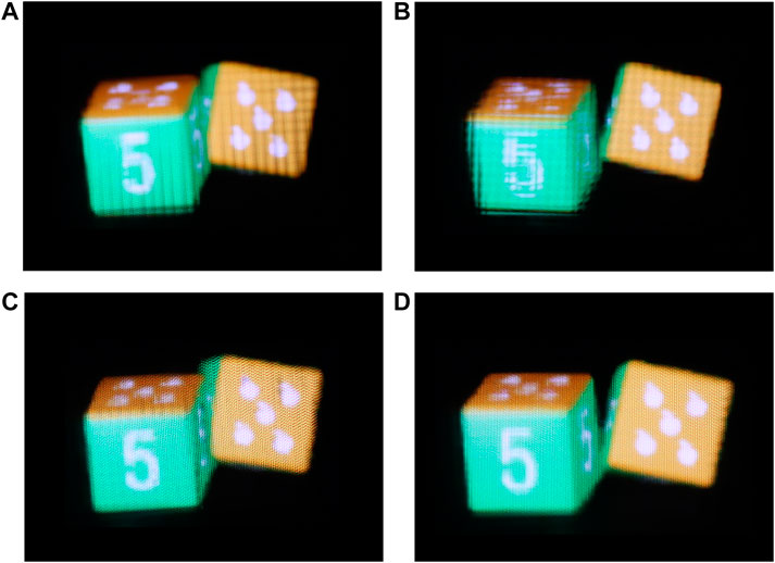
FIGURE 10. A comparison of optical reconstruction results for virtual capture scenes. SPOC: (A) left 7° viewing angle and (B) right 7° viewing angle. The proposed method: (C) left 7° viewing angle and (D) right 7° viewing angle.
The results of optical reconstruction suggest both methods are capable of solving the pseudoscopic problem. In this configuration, the left block is closer to the observer than the right block. As such, the perceived volume of the left block is also slightly larger, which indicates that both methods can restore spatial depth information to the original light field. However, the display quality of SPOC optical reconstructions was poor, as the left block exhibits splitting and blurring effects. This is closely related to the poor quality of the generated EIA. A comparison of Figures 10A and 10B also suggests the degree of splitting is not consistent for different viewing angles, which is primarily due to pixels from a single component originating from multiple EIs. As a result, the pixels are computationally independent and corresponding errors in the reference plane are also independent. Further observation indicated the splitting and blurring of the left block was more pronounced than in the right block, suggesting pixel position errors increase with decreasing distance between the object and the capture system. Since the left block is closer to the camera array, the errors caused by its reference plane have a greater impact. As seen in Figures 10A and 10B, optical reconstruction results produced by the proposed technique exhibit improved display effects. Numbers and patterns on the blocks are also displayed clearly and blurring effects are absent at multiple viewing angles. These results are consistent with the original scene as the proposed method does not artificially assume specific positions for the reference plane. Rather, it uses position differences for objects in the captured image for automatic optimization.
The performance of the proposed method was further compared with SPOC for varying capture densities, using virtual camera array sizes of 9 × 9, 13 × 13, 17 × 17, 23 × 23, 35 × 35, and 137 × 137. The EIA acquired at a density of 137 × 137 (the base image), the peak signal-to-noize ratio (PSNR), and the structural similarity (SSIM) index are shown for each algorithm in Figure 11.
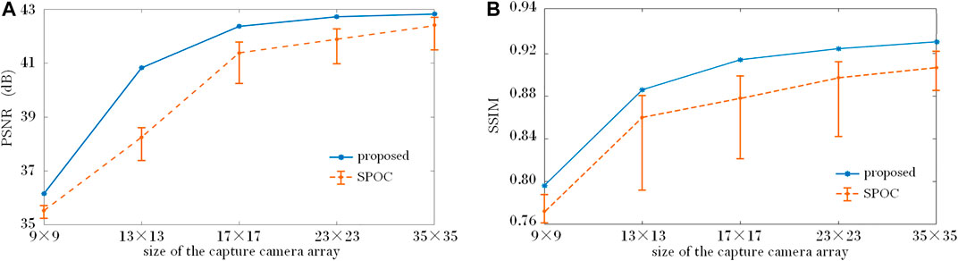
FIGURE 11. The influence of variations in capture camera density on image quality for generated elements, measured using (A) PSNR and (B) SSIM. The solid line indicates the proposed method, the dash line indicates the SPOC method. In the dash line, the upper short segment indicates the reference plane is at 100 mm, the central dot indicates the reference plane is at 80 mm, and the lower short segment indicates the reference plane is at 60 mm.
The plot indicates that PSNR and SSIM improved significantly for both algorithms as the density of cameras increased. However, the proposed technique produced better results at varying densities. For example, at the low density of 9 × 9, the difference between PSNR and SSIM for the two EIs was relatively small. This is because the distances between adjacent cameras and the area determined by the parallel captured light are large. Thus, the parallax angle between this area and the capturing camera varies significantly. Pixel values in this region of the captured image also varied widely as a result and serious pixel position errors were produced by both models. This effect demonstrates that the density of the acquiring cameras cannot be reduced indefinitely. The curve trend seen in the figure also suggests the proposed method improved PSNR and SSIM more quickly as the capture density increased. As the acquisition density increased to a certain level, changes in these values became relatively small. This is primarily because, as the capture density increases, the distance between adjacent cameras decreases and the area determined by the parallel light is reduced to the same region of the object. Corresponding pixel values in this area are then closer and the influence of pixel position errors is reduced, suggesting camera density does not need to be increased indefinitely. In addition, the reference plane also had a significant impact on the PSNR and SSIM of EIA calculated using SPOC. Specifically, these values improved as the reference plane was positioned closer to objects outside of the camera array. These experiments suggest the proposed technique can produce better EIA in complex scenes and sparse capturing configurations. In addition, the proposed technique does not require manual adjustment of the reference plane, which is more convenient.
Verification in Real Scenes
The capture system used for real scenes is shown in Figure 12. The focal length of each single camera is 8 mm, the resolution is 1981 × 1981, and the distance between adjacent cameras is 4 cm. The single-row array consists of 31 cameras fixed on a horizontal robotic arm, as shown in Figure 12A. During capture, the motor was used to move the array in the vertical direction with a step size of 4 cm. The final acquired image array is 21 × 31. The aircraft and tank models were placed forward and backward, the width of the models was both 10 cm, the distance between the geometric center of the aircraft and the tank model was ∼20 cm, the distance from the camera array to the aircraft was ∼1.5 m. The central perspective image for the scene is shown in Figure 12B, as the display system discussed previously was used to compare the effects produced by each technique. Capture system parameters required scaling using actual calculations, to ensure the scene subject fit completely within the display area. After zooming, the equivalent distance between adjacent cameras was 4 mm and the equivalent distance between the models and the camera array was 150 mm. When calculating the EIA, the equivalent distance between the display lens array and the acquisition camera array was set to 230 mm so that the display format of the LCD can be fully utilized, in this way, the reconstructed models were 60–100 mm form the display lens array. A comparison of EIA generated by SPOC and the proposed technique is shown in Figure 13.
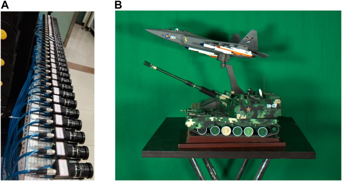
FIGURE 12. The actual scene capture system, including (A) the camera array and (B) the models.
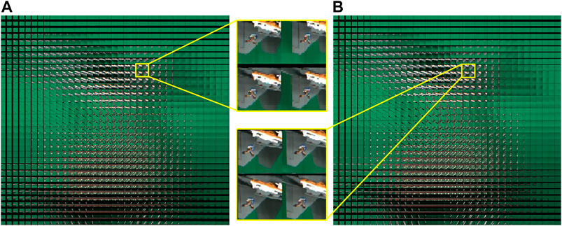
FIGURE 13. EIA generated by (A) SPOC and (B) the proposed method.
When generating the EIA with SPOC, the reference plane was positioned 150 mm away from the camera array. Close-up views in Figures 13A,B indicate the overall EIA content generated using each method was essentially the same. However, a careful comparison suggests the airplane icon was clearer in the EIs generated by the proposed technique. The edges of the wings are also smoother.
The generated EIA was used for actual display and the results demonstrate the superiority of the proposed technique, as shown in Figure 14. For example, the aircraft and tank models can be clearly displayed under different viewing angles. However, SPOC produced poor display effects in similar conditions. While the aircraft model is shown clearly, the tank exhibits obvious splitting. This is because the influence of the reference plane increased during sparse capture acquisition. The selection position for the reference plane was also closer to the aircraft model, so the impact of errors caused by inaccurate positioning was much smaller. Further inspection also suggests that splitting effects (such as the edge of the table) increased with distance from the reference plane. For instance, the aircraft tail icon is relatively clear using the proposed technique. The edges of the wing are also flatter and smoother. However, this same icon is significantly blurrier when displayed using SPOC.
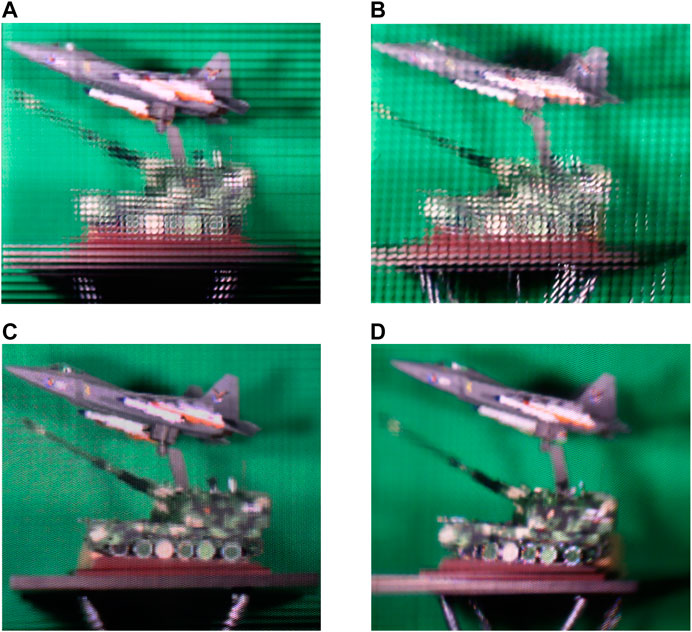
FIGURE 14. A comparison of optical reconstruction results for the real capture system. SPOC: (A) left 7° viewing angle and (B) right 7° viewing angle. The proposed method: (C) left 7° viewing angle and (D) right 7° viewing angle.
Combining virtual and real capture scenes indicates the proposed method can accurately calculate the required EIA under sparse capture conditions, which effectively improves the display of scenes with large field depths, making it more suitable for high-quality display systems.
The speed of the proposed method is affected by the density of cameras. In the experiments, the EIA was generated pixel by pixel, it costs about 10 min when the virtual camera array size is 23 × 23, and about 90 min when the virtual camera array size is 9 × 9. The main cost of the proposed method is to find the minimum value of
Conclusion
A new EIA generation technique was proposed to overcome pseudoscopic issues in sparse capturing environments. This approach is convenient and could reduce capturing costs in physical scenes. The distance between the displayed rays and adjacent captured rays in the same parallel light field components were calculated and used to determine contributions to the generated image. Errors under the same sparse capture conditions were analyzed, and pixel position errors were determined by comparing the similarity of areas defined by the parallel capture rays. Experiments using both virtual scenes of bricks and real scenes of aircraft and tank models verified the effectiveness of the proposed method. The SSIM and PSNR values of the virtual scenes showed that the proposed method can improve the accuracy of generated EIA. Optical reconstruction results showed the EIA generated using the proposed model can effectively improve displays, making it more suitable for scenes with large field depths. In addition, this technique does not require manual adjustment of the reference plane or any other parameters, which simplifies the practical operation.
Data Availability Statement
The original contributions presented in the study are included in the article/Supplementary Material, further inquiries can be directed to the corresponding authors.
Author Contributions
Conceptualization, YH and XJ; Methodology, ZY and XY; Software, ZY and XY; Validation, TJ; Formal Analysis, SC; Writing—Original Draft Preparation, ZY and ML; Writing—Review and Editing, YH and XY; Resources, JZ; Funding Acquisition, XY All authors have read and agreed to the published version of the manuscript.
Funding
This work was partly supported by the National Key Research and Development Program of China (2017YFB1104500), National Natural Science Foundation of China (61775240), and Foundation for the Author of National Excellent Doctoral Dissertation of the People’s Republic of China (201432).
Conflicts of Interest
Author JZ was employed by the company Jiangsu North Huguang Opto-Electronics Co., LTD. The remaining authors declare that the research was conducted in the absence of any commercial or financial relationships that could be construed as a potential conflict of interest.
References
2. Ives HE. Optical properties of a lippmann lenticulated sheet. J Opt Soc Am (1931) 21(3):171–6. doi:10.1364/josa.21.000171
3. Okano F, Hoshino H, Arai J, Yuyama I. Real-time pickup method for a three-dimensional image based on integral photography. Appl Opt (1997) 36(7):1598–603. doi:10.1364/ao.36.001598
4. Martínez-Corral M, Javidi B, Martínez-Cuenca R, Saavedra G. Formation of real, orthoscopic integral images by smart pixel mapping. Opt Exp (2005) 13(23):9175–80. doi:10.1364/opex.13.009175
5. Shin D-H, Lee B-G, Kim E-S. Modified smart pixel mapping method for displaying orthoscopic 3D images in integral imaging. Opt Lasers Eng (2009) 47(11):1189–94. doi:10.1016/j.optlaseng.2009.06.004
6. Navarro H, Martínez-Cuenca R, Saavedra G, Martínez-Corral M, Javidi B. 3D integral imaging display by smart pseudoscopic-to-orthoscopic conversion (SPOC). Opt Exp (2010) 18(25):25573–83. doi:10.1364/OE.18.025573
7. Xiao X, Shen X, Martinez-Corral M, Javidi B. Multiple-planes pseudoscopic-to-orthoscopic conversion for 3D integral imaging display. J Display Technol (2015) 11(11):921–6. doi:10.1109/jdt.2014.2387854
8. Deng H, Wang Q, Li D. Method of generating orthoscopic elemental image array from sparse camera array. Chin Opt Lett (2012) 10(6):061102–4. doi:10.3788/col201210.061102
9. Chien L-C, Kim J, Lee S-D, Jung J-H, Lee B, Wu MH. Real-time pickup and display integral imaging system without pseudoscopic problem. Int Soc Optics Photon (2013) 8643:864303. doi:10.1117/12.2007369
10. Jung JH, Kim J, Lee B. Solution of pseudoscopic problem in integral imaging for real-time processing. Opt Lett (2013) 38(1):76–8. doi:10.1364/OL.38.000076
11. Piao Y, Zhang M, Lee J-J, Shin D, Lee B-G. Orthoscopic integral imaging display by use of the computational method based on lenslet model. Opt Lasers Eng (2014) 52:184–8. doi:10.1016/j.optlaseng.2013.06.012
12. Zhu Y, Sang X, Yu X, Wang P, Xing S, Chen D, et al. Wide field of view tabletop light field display based on piece-wise tracking and off-axis pickup. Opt Commun (2017) 402:41–6. doi:10.1016/j.optcom.2017.05.056
13. Wang Z, Lv G, Feng Q, Wang A. A fast-direct pixel mapping algorithm for displaying orthoscopic 3D images with full control of display parameters. Opt Commun (2018) 427:528–34. doi:10.1016/j.optcom.2018.06.067
14. Liu ZS, Deng H, Li JJ, Deng H, Lv GJ, Fan J, et al. Light field resampling method for elemental image array generation of integral imaging. J Soc Inf Display (2020) 28(8):705–12. doi:10.1002/jsid.865
15. Zhang H-L, Deng H, Ren H, Yang X, Xing Y, Li D-H, et al. Method to eliminate pseudoscopic issue in an integral imaging 3D display by using a transmissive mirror device and light filter. Opt Lett (2020) 45(2):351–4. doi:10.1364/OL.45.000351
Keywords: three-dimensional display, integral imaging, pseudoscopic-to-orthoscopic conversion, sparse capturing, elemental image
Citation: Huang Y, Yan Z, Jiang X, Jing T, Chen S, Lin M, Zhang J and Yan X (2021) Performance Enhanced Elemental Array Generation for Integral Image Display Using Pixel Fusion. Front. Phys. 9:639117. doi: 10.3389/fphy.2021.639117
Received: 08 December 2020; Accepted: 08 February 2021;
Published: 08 April 2021.
Edited by:
Lorenzo Pavesi, University of Trento, ItalyCopyright © 2021 Huang, Yan, Jiang, Jing, Chen, Lin, Zhang and Yan. This is an open-access article distributed under the terms of the Creative Commons Attribution License (CC BY). The use, distribution or reproduction in other forums is permitted, provided the original author(s) and the copyright owner(s) are credited and that the original publication in this journal is cited, in accordance with accepted academic practice. No use, distribution or reproduction is permitted which does not comply with these terms.
*Correspondence: Xiaoyu Jiang, amlhbmd4aWFveXUyMDA3QGdtYWlsLmNvbQ==; Xingpeng Yan, eWFueHAwMkBnbWFpbC5jb20=