On the Time Transition Between Short- and Long-Time Regimes of Colloidal Particles in External Periodic Potentials

The dynamics of colloidal particles at infinite dilution, under the influence of periodic external potentials, is studied here via experiments and numerical simulations for two representative potentials. From the experimental side, we analyzed the motion of a colloidal tracer in a one-dimensional array of fringes produced by the interference of two coherent laser beams, providing in this way an harmonic potential. The numerical analysis has been performed via Brownian dynamics (BD) simulations. The BD simulations correctly reproduced the experimental position- and time-dependent density of probability of the colloidal tracer in the short-times regime. The long-time diffusion coefficient has been obtained from the corresponding numerical mean square displacement (MSD). Similarly, a simulation of a random walker in a one dimensional array of adjacent cages with a probability of escaping from one cage to the next cage is one of the most simple models of a periodic potential, displaying two diffusive regimes separated by a dynamical caging period. The main result of this study is the observation that, in both potentials, it is seen that the critical time $t^{\text{*}}$, defined as the specific time at which a change of curvature in the MSD is observed, remains approximately constant as a function of the height barrier $U_0$ of the harmonic potential or the associated escape probability of the random walker. In order to understand this behavior, histograms of the first passage time of the tracer have been calculated for several height barriers $U_0$ or escape probabilities. These histograms display a maximum at the most likely first passage time $t^{\prime }$, which is approximately independent of the height barrier $U_0$, or the associated escape probability, and it is located very close to the critical time $t^{\text{*}}$. This behavior suggests that the critical time $t^{\text{*}}$, defining the crossover between short- and long-time regimes, can be identified as the most likely first passage time $t^{\prime }$ as a first approximation.

1 Introduction

A colloidal particle undergoing Brownian motion presents deviations from pure diffusion when such a particle interacts with an external potential or when it moves in a crowded environment. Some examples of crowded environments that affects colloidal motion include the colloidal motion of proteins or organelles in the interior of a cell [1–3], the motion of a tracer particle in complex fluids [4–9] and colloidal motion near the glass transition [10, 11]. On the other hand, examples of external fields that affect Brownian motion are electric and magnetic fields [12], gravitational forces [13–15] and optical manipulation induced by light [16, 17]. The diffusion of tracers in periodic, quasiperiodic, and random external potentials has been also studied in underdamped and overdamped conditions theoretically, experimentally and via numerical simulations [18–21].

On the other hand, the main effect of external potentials, or crowded environments, in colloidal dynamics is to promote the appearance of time regimes in which particles might slow down (subdiffusion) or speed up (superdiffusion) their motion as compared with normal diffusion. Generally speaking, a colloidal particle senses its environment when it moves in Brownian motion. As a result, each time regime is related to a particular length scale. The dynamics of a colloidal tracer provides useful information about the concentration of other colloidal macromolecules, the degree of coupling between the tracer and an applied external field, as well as the competition between the energy associated to the external potential and the thermal energy [4, 10, 17, 22].

One of the most simple cases where the appearance of different time regimes has been reported, due to the interaction of a particle with an inhomogeneous external field, is a one dimensional periodic potential interacting with a 2D colloidal suspension [23–25]. Such a system has many advantages: it can be simulated via BD simulations and can be experimentally realized by using the interference of two coherent beams, providing energy barriers of height close to the thermal energy, for laser powers smaller than 1 W [26]. A colloidal particle interacting with a periodic potential presents three time regimes related with different effects: free diffusion with a linear mean square displacement can be observed at short times; a plateau in the mean square displacement associated to “caging,” produced by the existence of an energy barrier, can be seen at intermediate times; and a hopping motion of the colloidal tracer between adjacent periodic fringes in a second diffusive regime can be observed at long times [23, 24]. Similarly, a random walker simulation have been used extensively to simulate Brownian motion [27–29]. In this type of simulations, the trajectories are obtained from random numbers just as the BD simulations, but the displacement is chosen more simply, not derived from a force. Thus, the confinement is introduced as a spatial condition of no escaping from a region. The height barrier effect is then introduced as a cage-to-cage hopping probability. This allow us to observe a process similar to that displayed by a Brownian particle in a periodic potential, showing a short- and a long-time diffusive regime as a function of time. Note, however, that in the random walker simulation the particle is free to move within the cage in contrast to the cosine-like potential used in the Brownian dynamics approach.

It is important to note that the three time regimes presented above mainly depend on the periodicity of the external potential and the amplitude of the energy barrier, or the hopping probability, and they can extend over several time decades [23, 24, 30]. For example, the short time regime is related with free diffusion and thus is limited to the time the particle takes to diffuse at the bottom part of the potential; the extension of the plateau region is directly related with the amplitude of the potential, and finally the long time diffusion results of a balance between hopping time, and thus related with the amplitude of the potential, and the periodicity of the potential. Furthermore, this potential had been also studied for mean first passage time calculations, giving theoretical predictions for the ratio between the diffusion coefficients associated with its dynamics [31]. In such a scenario, colloidal dynamics can be described by the ratio between the short- and long-time diffusion coefficients [23]. Other quantities of interest are the time at which the caged motion begins, and the time at which the hopping motion starts. As indicated before, the phenomenology found in this potential can be mapped to several other situations. Thus, for complex fluids, the long-time diffusion coefficient is related to the zero shear viscosity [22], whereas the glass transition is related to the so-called alpha relaxation [32]. Despite numerous theoretical, simulation, and experimental studies that had been performed since last century, a complete characterization of the prediction of the short- and long-times diffusion coefficient, using available theoretical models, as well as the study of the critical caging time and the distribution of hoping times, is still lacking.

In this work, the dynamics of a colloidal particle in periodic potentials is studied by using experiments and simulations, focusing in the short- and long-times dynamics. We are particularly interested in the behavior of the critical time at which the MSD changes its curvature when the caging effect appears, and in the distribution of hoping times between adjacent periodic cells. We also compare our results with available theoretical predictions. Our results give a full characterization of the phenomena in terms of energy barriers and the associated dynamical caging, providing a simple model to understand the colloidal dynamics under different, but equivalent scenarios.

2 Model and Methods

2.1 Experimental Methods

The experimental system consists of a highly dilute water suspension of 1 µm polystyrene spherical particles (Thermo Scientific) confined between one microscope slide and a cover slip. The sample has been prepared by following the procedure described by Carbajal-Tinoco et al. [33].

The experimental set up for the light potential is based on the interference of two beams in the plane of the sample, which produces a periodical array of bright fringes of a specific width. This experimental setup has been fully described elsewhere [34], here we only discuss the main points. The laser beam used has a spectral width <200 kHz (Azur Light Systems) and range powers between 40 and 500 mW. A half-wave plate and a fixed polarizer allow us to vary the input power by rotating the half-wave plate. The laser beam passes through a beam splitter, which divides the beam in two with the same laser power. Both beams are directed into a prism mirror that reflects the beams parallel each other. The prism is mounted on a base that can be moved manually to change the distance between the beams. A spherical lens initializes the convergence of both beams in order to produce the interference pattern in the focal plane of the lens. The distance of separation between the beams determines the angle ψ of incidence, which defines the periodicity of the intensity pattern. However, it also changes the effective focal distance of the lens due to spherical aberration. Thus, a focusing lens is mounted on a moving stage to correct such effect. This interferometer is coupled using a dichroic mirror to an inverted microscope (OLYMPUS U-LH100-3) with a 60X objective and numerical aperture 0.6, that allows us to obtain high quality clear field images in order to get the time evolution of the system.

The interference of the coherent beams produce an intensity pattern expressed as [35].

$I\left(x\right)=2I_0\left\{1+\cos \left[2kx\sin \left(\psi /2\right)\right]\right\}{e}^{-2{\left(x/R\right)}^2{\cos }^2\left(\psi /2\right)}(1)$

where $I_0$ is the intensity of each beam, $k=2\pi /{\lambda }_0$, with ${\lambda }_0=488\text{}\text{}\text{}nm$ the incident beam wavelength and R the laser beam radius. As it can be seen here, the periodicity of the distribution of light is directly related to the angle ψ. For our experimental conditions, the set-up is able to produce fringes between 1.3 and 6.0 μm by varying the position of the prism mirror. As shown before [34], if the periodicity of the light distribution is larger than the size of the particle, such a distribution produces a periodical potential with the same periodicity, where the bright fringes corresponds to the minima in the potential. For this study, the periodicity of the distribution of light was set to 1 µm. Similarly as in optical tweezers, instead of estimating the external potential using the distribution of light and some model of interaction of light with an spherical particle [36, 37], in this work the external potential was calibrated comparing the experimental values of the MSD with those resulting from the Brownian dynamics simulation.

The time evolution of the system has been recorded by using standard video equipment at 30 frames per second, giving an experimental time resolution of 0.033 s. The tracking of the particles has been performed by using Trackpy [38], which implements and extends the Crocker-Grier algorithm in Python language [39]. Furthermore, by placing neutral density filters on the lens of the recording camera, the intensity profile generated by the interference of the beams can be imaged, and thus the spatial position of the minima has been estimated. This is very helpful for the calculation of the spatial-dependent statistical properties. It is important to note that we analyze the trajectories of particles at the center of the field of view since the spatial distribution of light is not homogeneous at the edges due to the Gaussian envelope. This ensures that the variation of the intensity in the region of interest is less than 10%, where the particles interact with a similar external potential. The area in the region of interest corresponds to 1908.5 µm², and a total of 2 h of recording, divided in three videos, were analyzed, giving almost 2,000 trajectories. However, most of them are very short, corresponding to particles that remained within the region of interest only for a few frames. Such trajectories contributed to the short time dynamics, and thus giving a reliable quantification of the mean squared displacement at short times as well as of the density of probability of displacements. However, the long time dynamics lacks of statistics as only a few particles remain during the total duration of the video. The duration of each experiment was defined due to the presence of a small drift in the laser beam, producing a motion of the fringes in one direction. We found that during intervals of 20 min there is a very small variation of the position of the fringes, giving confidence in the position of the fringes. Fringes were also found to vibrate due to external mechanical noise, even tough the experiment was performed on an isolated optical table. Once we get the trajectories of the particles we are able to calculate the total average displacement and the mean square displacement of all trajectories of particles in a time interval. A schematic representation of the protocol we have described is shown in Figure 1.

FIGURE 1

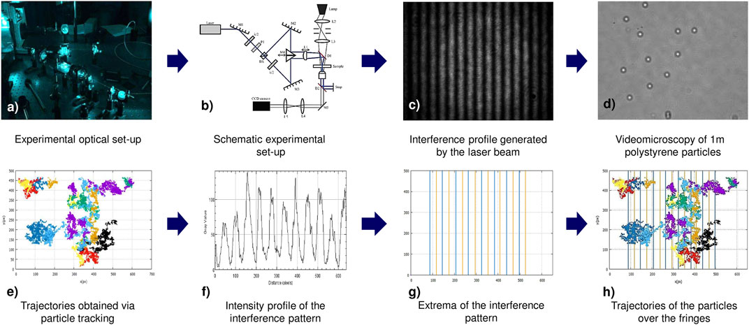
FIGURE 1. (Color online): Experimental measurement protocol of the dynamic properties of spherical tracers in periodic cosine-like potentials: (A) long exposure photograph showing the light path producing the periodic distribution of light; (B) schematic representation of the experimental set-up; (C) light intensity profile generated experimentally; (D) typical bright field images of spherical tracers interacting with the external field; (E) trajectories obtained from the experiment using Trackpy; (F,G) the maxima and minima of the periodic potentials are estimated from the bright and dark regions displayed in the panel (C); and (H) the density of probability is calculated from the information obtained from the trajectories of the particles over the fringes.

2.2 Theoretical Model and Brownian Dynamics Simulations

In this work, we consider that a tracer particle is under the influence of a periodic cosine potential of the form:

$U\left(x,U_0,L\right)=U_0\left(1-\cos \left(\frac{2\pi x}{L}\right)\right)(2)$

where $U_0$ and L are the amplitude and periodicity of the external potential, respectively.

The Brownian dynamics simulations were performed using the method proposed by Ermak and McCammon without hydrodynamic interactions [40]. As the experimental particle concentration is very low, we consider a single particle in a one-dimensional simulation box with periodic boundary conditions along the $x-axis$. In the $y-axis$, the experimentally developed field is constant, and thus we restrict the simulation to a one dimensional problem. In the Brownian dynamics simulations, the position of the particle at time $t+dt$ is calculated from the previous position at time t by using the equation:

$x\left(t+dt\right)=x\left(t\right)+\frac{D_{0}F\left(x\left(t\right)\right)dt}{k_{B}T}+R\left(dt\right)(3)$

where $D_0$ is the translational diffusion coefficient of the particle at short-times, $F\left(x\right)=-\frac{dU\left(x\right)}{dx}$ is the force that the particle experiences due to the external periodic potential $U\left(x\right)$, and $R\left(dt\right)$ is a random displacement, having a normal distribution with zero mean value and variance $2D_{0}dt$, fulfilling the so-called fluctuation-dissipation theorem. In Brownian dynamics simulations, the magnitude of the time step $dt$ is crucial. If it is too short, the computational time can increase significantly. If it is too large, the stochastic differential equation can display incorrect values of the dynamic properties of the system. The use of a single tracer under the influence of an external field allowed us to utilize a time step of 3 µs. Let us note here that the experimental time resolution is an order of magnitude larger. Such time step allowed us to reproduce the analytic mean square displacement of the Brownian harmonic oscillator with an error less than 1 percent for a wide range of spring constants [41]. In a typical Brownian dynamics simulation a maximum $N_{\max }=1\times {10}^{11}$ times steps have been performed, which is equivalent to a total time of $3\times {10}^{5}s$. Once the positions of the tracer are known as a function of time, and assuming that the statistical properties do not depend on the initial time, the mean square displacement has been calculated as:

$MSD\left(t_j\right)=\frac{1}{N_{\max }-j}{\displaystyle \sum }_{i=1}^{N_{\max }-j}{\left[x\left(t_i+jdt\right)-x\left(t_i\right)\right]}^2(4)$

where $t_i=idt$.

On the other hand, Bellour et. al. [9]. have proposed the following functional form to fit the MSD of tracer particles in worm-like micelle solutions:

$MS{D}^{Bellour}\left(t\right)=2{\delta }^2{\left(1-\exp \left\{-{\left(\frac{D_{0}t}{{\delta }^2}\right)}^{\alpha }\right\}\right)}^{\frac{1}{\alpha }}\left(1+\frac{D_{M}t}{{\delta }^2}\right)(5)$

This equation correctly describes the above mentioned dynamical regimes: short time diffusion within the network of micelles, cage effect at intermediate times, and hopping motion due to breaking of the living polymer giving a second linear regime at long times and thus can be used as a model to estimate some parameters characterizing the MSD of particles in periodical potentials. $D_0$ is the short time diffusion coefficient, which can be approximated as $D_0\approx k_{B}T/6\pi \eta a$ according to the Stokes-Einstein relationship as a first approximation, where $k_{B}T$ is the thermal energy, η is the solvent viscosity, and a is the particle’s radius. Experimentally, the short time diffusion coefficient $D_0$ is frequently different from $k_{B}T/6\pi \eta a$ given that $D_0$ also contains information regarding inter-particle interactions and wall-particle interactions. ${\delta }^2$ is related to the amplitude of the MSD within the cage and thus, it is usually called the cage size. Notice that in general $2{\delta }^2$ is not equal to the periodicity L of our oscillatory potential. $D_M$ corresponds to the long time diffusion coefficient, which in our system characterizes the hopping of the tracer between fringes as a function of time in our periodic system. Finally, α is a parameter related to the smoothing of the transition between short times and the caging, and it has a value close to 0.25 in worm-like micelle solutions [5]. The Bellour parametrization was originally proposed by considering that a tracer immersed in a semidilute solution of worm-like micelles was describing three different dynamic regimes in one dimension: 1) at short times the dynamics is Brownian, that is, $MSD\left(t\right)=2D_{0}t$, where $D_0$ is the local diffusion coefficient; 2) at intermediate times, the MSD remains constant for a given time interval, in such a way that $2{\delta }^2$ is the value of the MSD at the inflexion point; and 3) at long-times the motion becomes diffusive again and the long-time diffusion coefficient corresponds to the macroscopic viscosity of the solution. Thus, the starting point to describe this phenomenology is to hypothesize that the particle is under the influence of a harmonic potential. As a result, the MSD cannot grow indefinitely but reaches a plateau:

$MSD\left(t\right)=\frac{2k_{B}T}{k_{spring}}\left(1-\exp \left(-\frac{k_{spring}t}{\gamma }\right)\right)(6)$

where $D_0=\left(k_{B}T\right)/\gamma$. By assuming that $k_{spring}=\left(K_{B}T\right)/{\delta }^2$, it is possible to write

$MSD\left(t\right)=2{\delta }^2\left(1-\exp \left(-\frac{D_{0}t}{{\delta }^2}\right)\right)(7)$

If the exponential is linearized, it is easy to see that at short times $MSD\left(t\right)=2D_{0}t$, whereas at long times a plateau is reached at $2{\delta }^2$. One simple form in which the MSD can reach the physical limit $MSD\left(t\right)=2D_{M}t$ is by multiplying the analytical MSD associated to a Brownian particle under the influence of a harmonic potential by the term $1+\left(D_{M}t\right)/{\delta }^2$:

$MSD\left(t\right)=2{\delta }^2\left(1-\exp \left(-\frac{D_{0}t}{{\delta }^2}\right)\right)\left(1+\frac{D_{M}t}{{\delta }^2}\right)(8)$

Even though this last equation is able to reproduce the MSD of a tracer immersed in a semidilute solution of worm-like micelles at short- and long-times, in general fails to describe the onset of the plateau around the inflexion point. Thus, Bellour proposed to add a parameter α in order to adjust the onset of the experimental plateau of the MSD. As one can appreciate here, the same basic arguments employed by Bellour in this heuristic derivation of Eq. 5 can be used in the case of the systems studied here.

Another methodology to characterize the dynamical behavior of a particle in hindered motion is related with the logarithmic derivative, that corresponds to the temporal behavior of the exponent γ in $MSD\propto t^{\gamma }$. As such, a numerical calculation can be complex due to the experimental noise. We used here a more direct approach by fitting the experimentally obtained MSD to the Bellour model. Afterwards, these fitted parameters have been used in the analytic calculation of the logarithmic derivative of Eq. 5.

In order to calculate the long-time diffusion coefficient $D_M$ theoretically, we consider that this quantity corresponds to the effective diffusion coefficient of a hopping Brownian particle that moves a distance L in the presence of a periodic external potential with periodicity L. In such a scenario [42],

$D_M=D_{eff}=\frac{1}{2}{k}_{escape}{L}^2(9)$

where $k_{escape}=1/{\tau }_{escape}$ is the escape or hopping rate of the Brownian particle. Let us define the mean first passage time (MFPT) ${\tau }_{MFPT}$ as the average time a Brownian particle needs to reach the separatrix manifold for the first time, when was located initially at a position $x_0$ inside the initial domain of attraction. At large height barriers, the MFPT ${\tau }_{MFPT}\left(x_0\right)$ becomes essentially independent of the starting point, that is, ${\tau }_{MFPT}\left(x_0\right)$ is approximately the same for all starting configurations away from the immediate neighborhood of the separatrix. If the probability of crossing the separatrix to the right or to the left equals one half, the total escape time equals to two times the MFPT, and the escape or hopping rate of the Brownian particle can be written as:

$k_{escape}=\frac{1}{2{\tau }_{MFPT}}(10)$

Thus, Eq. 9 can be written in terms of the MFPT as:

$D_M=\frac{1}{4{\tau }_{MFPT}}{L}^2(11)$

On the other hand, the diffusion coefficient of a Brownian particle in the presence of a periodic potential, according to the Kramers approach in the overdamped limit, can be written as [43].

$D_M^{Kramers}=\frac{w_0{w}_b{L}^2}{2\pi \gamma }\exp \left\{-\frac{E_b}{k_{B}T}\right\}(12)$

where $E_b=V\left(x_{\max }\right)-V\left(x_{\min }\right)$, $w_0^2=V^{\prime \prime }\left(x_{\min }\right)$, $w_b^2=V^{\prime \prime }\left(x_{\max }\right)$, and $D_0=\frac{k_{B}T}{\gamma }$. If we chose

$V\left(x\right)=U_0\left(1-\cos \left(\frac{2\pi x}{L}\right)\right)(13)$

$x_{\min }=0$, $x_{\max }=\frac{L}{2}$, and $E_b=2U_0$, Eq. 12 can be written as:

$\frac{D_M^{DF}}{D_0}=\frac{2\pi U_0}{k_{B}T}\exp \left\{\frac{-2U_0}{k_{B}T}\right\}(14)$

which is the Dalle-Ferrier et al. [23] (DF) formula for a Brownian particle in a periodic cosine potential. According to Lifson and Jackson [30], the ratio of the long-time diffusion coefficient of a Brownian particle in the presence of a periodic potential $U\left(x\right)$ can be written as:

$\frac{D_M^{LJ}}{D_0}=\frac{1}{\langle \exp \left\{U\left(x\right)/\left(k_{B}T\right)\right\}\rangle \langle \exp \left\{-U\left(x\right)/\left(k_{B}T\right)\right\}\rangle }(15)$

where the brackets $\langle \dots \rangle$ indicate the average over the unit cell. This result was obtained subsequently by several authors using different routes, mainly based in solving the mean first passage time problem using the one-dimensional Smoluchowski equation.

The corresponding MFPTs can be obtained by equating Eq. 11 with either Eq. 12 or Eq. 15 to yield:

${\tau }_{MFPT}^{DF}=\frac{1}{4\pi }{\tau }_0\frac{k_{B}T}{U_0}\exp \left\{\frac{2U_0}{k_{B}T}\right\}(16)$

and

${\tau }_{MFPT}^{LJ}=\frac{1}{2}{\tau }_0\langle \exp \left\{U\left(x\right)/\left(k_{B}T\right)\right\}\rangle \langle \exp \left\{-U\left(x\right)/\left(k_{B}T\right)\right\}\rangle (17)$

where

${\tau }_0=\frac{L^2}{2D_0}(18)$

is the time that a particle needs to move a distance L in pure Brownian motion, that is, in the absence of any external potential, when the diffusion constant of the particle is $D_0$. As it is shown below, the Kramers escape time resembles more to the escape times predicted by the Lifson-Jackson prescription and the Brownian dynamics simulations at high values of $U_0$. On the other hand, notice that in the absence of an external potential (that is, in pure Brownian motion) the ${\tau }_{escape}^{LJ}$ reduces to ${\tau }_0$ as expected, whereas the ${\tau }_{escape}^{DF}$ diverges to an infinite time. In addition, note that in the Lifson-Jackson approach the long-time diffusion coefficient $D_M$ requires a numerical integration, whereas the Dalle-Ferrier formula is completely analytical.

2.3 Random Walker

A random walker simulation follows a similar recipe to obtain a trajectory as the Ermak and McCammon algorithm, however the choice of the displacement is generated randomly either following a distribution, or with a defined step size but without specification of the force or diffusion coefficient [27–29]. In our case, such distribution is flat of fixed width $\delta x$, instead of the typical Gaussian distribution found experimentally and also simulated in the BD protocol. The time scaling constant is not fixed and can be chosen arbitrarily. In our case it was fixed to a value of $\delta t=0.1s$. The evolution of density of probability $\rho \left(x,t\right)$ of finding a tracer at the position x at time t given that a $t=0$ the particle was located at $x=0$ produces a Gaussian distribution after a few time steps, thus becoming dynamically equivalent to a BD simulation after such time (see Figure 2), as expected. As the distribution if perfectly Gaussian, it is expected also that higher moments are also equivalent. If the width of the distribution δ and the time scaling constant are chosen conveniently, this walker can reproduce the diffusion coefficient, $D_0$, of the BD simulations at short times. Thus, we can conclude that the implemented random walk simulation follows the most simple selection of displacements between time steps. This naive selection gives an important difference between the BD and the random walk at short times, as the probability function of displacements is not Gaussian in the first few lag times. However, this function evolves to a Gaussian distribution function, and thus not only the second moment but also higher moments are equivalent and indistinguishable from the BD. Thus, at large times both simulations are dynamically equivalent for a free particle.

FIGURE 2

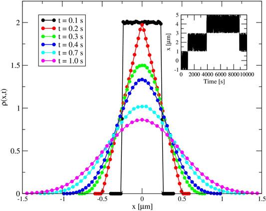
FIGURE 2. (Color online) $\rho \left(x,t\right)$ at different times for the random walker simulation. For $t=0.1$ s the step distribution is recovered, whereas the probability evolves to a Gaussian after a few steps. Inset: Representative trajectory obtained from the simulation, showing the caging effect and a hopping effect.

In order to introduce the cage effect, the particle is located inside a periodic cell of length $L^{\#}$ with potential barriers of vanishing small width at the boundaries. Then the random walker is free to move within the cage, undergoing random steps with displacement probability. The particle can cross the cell boundary to move to an adjacent cage with a transition probability p if a given generated step is out of the cage. The success event gives a transition to the neighboring cage, whereas a failure reflects the step to keep the particle inside the cage. Thus, decreasing the transition probability gives a higher amount of events before a success one, effectively producing confinement within the cell for a given time. Inset in Figure 2 shows a typical trajectory for a random walker in a cage of size 2 µm and transition probability 0.001, showing the typical confinement and several transitions within the simulation time. A transition probability of zero leads to total confinement, and the walker is unable to escape from the cage. In the opposite, free diffusion is found for a transition probability of 1. Despite that, after few time steps the random walker simulation and the BD simulation are dynamically equivalent for free particles, the case of a caged particle, either in the periodic potential or in a cage with a probability of transition, is different. In this case, a direct computation of the probability density within a unity cell would show that the random walker is almost free within the cage, giving a probability density almost constant within the cage, whereas the presence of the continuous potential in the BD would produce a more complex scenario. Despite this, and as shown here, choosing properly the parameters of the random walker, the evolution of the MSD is equivalent.

The random walker model is also useful to study the typical mean first passage time problem, that will be used later to analyze our results in terms of the distribution of escape times. However, as in this case the particle either cross the barrier or not, in principle, the random walker undergoes escaping processes, characterized by an escape time ${\tau }_E$, instead of the mean first passage time. By now it is important to highlight the relation between the escape time problem and the parameters of such stochastic model. Consider first that the potential that can be modeled using the random walker is a flat bottom well with delta barriers as frontiers. When considering the simple case of a flat potential with perfectly absorbing barriers, the mean first passage time, equivalent to escape time only in this case, was found to be $L^{\#2}/\left(16D_0\right)$, as expected from this simple model [44]. By including a transition probability p, the escape time can be written as $L^{\#2}/\left(16D_{0}p\right)$, which provides a definition of the long time diffusion coefficient $D_M$ similar to that used in the BD simulation case

$D_M=\frac{1}{2{\tau }_E}{L}^{\#2}(19)$

where $D_M=8D_{0}p$. In such a scenario, the escape time is twice the mean first passage time, which is consistent with a 1/2 probability of jumping to the next cage per event.

3 Results and Discussion

3.1 Short Time Dynamics

In order obtain the short time diffusion coefficient $D_0$ of a tracer, and the amplitude of the periodic potential $U_0$ in our experiment, we measured the mean square displacements along the $y-$ and $x-axis$ directions as a function of time. Given that along the y-axis there is not an applied external field, the tracer experiences free diffusive Brownian motion. Using the total mean square displacement (associated to the free diffusion in the $y-$ and $x-axis$ directions), the short time diffusion coefficient was found to be $D_0=1.8\times {10}^{-13} m^2/s$, which in turn is used in our Brownian dynamics simulations, allowing us to reproduce the observed experimental behavior as it is shown in Figure 3. The reduction of $D_0$ is about 35% with respect the Stokes-Einstein equation for free diffusion in the bulk, in accordance with previous results for a similar geometry confinement [45]. Some deviations from these value are expected experimentally as the separation between glass plates varies within the sample, but deviations in $D_0$ are also expected to be small and thus does not greatly affect the comparison between experimental and numerical results. A direct comparison with the experimental mean square displacement measured in the x-axis allowed us to fit the maximum height of the periodic potential, resulting in the numerical value of $U_0=1.33k_{B}T$. Brownian dynamics simulations of the tracer with the above values of $D_0$ and $U_0$ yielded a numerical mean square displacement that correlate very well with experimental measurements in the x-axis, as it is shown in Figure 3. Some deviations from the perfect linear relation was found in the experimental MSD and associated with the small vibrations reported above. As only a few particles remain withing the field of view for more than 100 s, the long time dynamics is also found to be affected by statistical noise.

FIGURE 3

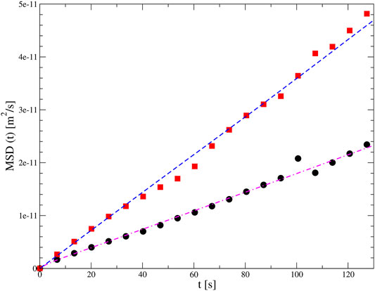
FIGURE 3. (Color online): Mean square displacement MSD(t) of a spherical tracer as a function of time. The red solid squares and the blue dashed line correspond to the total mean square displacement (associated to the free diffusion in the $y-$ and $x-axis$ directions) associated to experimental and Brownian dynamics results, respectively, in the absence of an external field. The black solid circles and the magenta dot-dashed line correspond to the MSD(t) in the $x-axis$ associated to experimental and Brownian dynamics results, respectively, in the presence of a periodic cosine-like external field.

A more stringent test for the estimated value of $U_0$ parameters (fitted via the experimental mean square displacement) is to observe if it is able to predict other microscopic time dependent properties such as the density of probability $\rho \left(x,t\right)$ of finding a tracer at the position x at time t given that at $t=0$ the particle was located at $x=0$. This quantity, obtained from experiments and Brownian dynamics calculations, is shown in Figure 4. The behavior of $\rho \left(x,t\right)$ in the presence of a periodic external field is shown in panels (a) and (c), whereas $\rho \left(x,t\right)$ in the absence of an external field is displayed in panels (b) and (d). In general, good agreement between the experimental and Brownian dynamics data is observed either in presence or in the absence of the periodic external field.

FIGURE 4

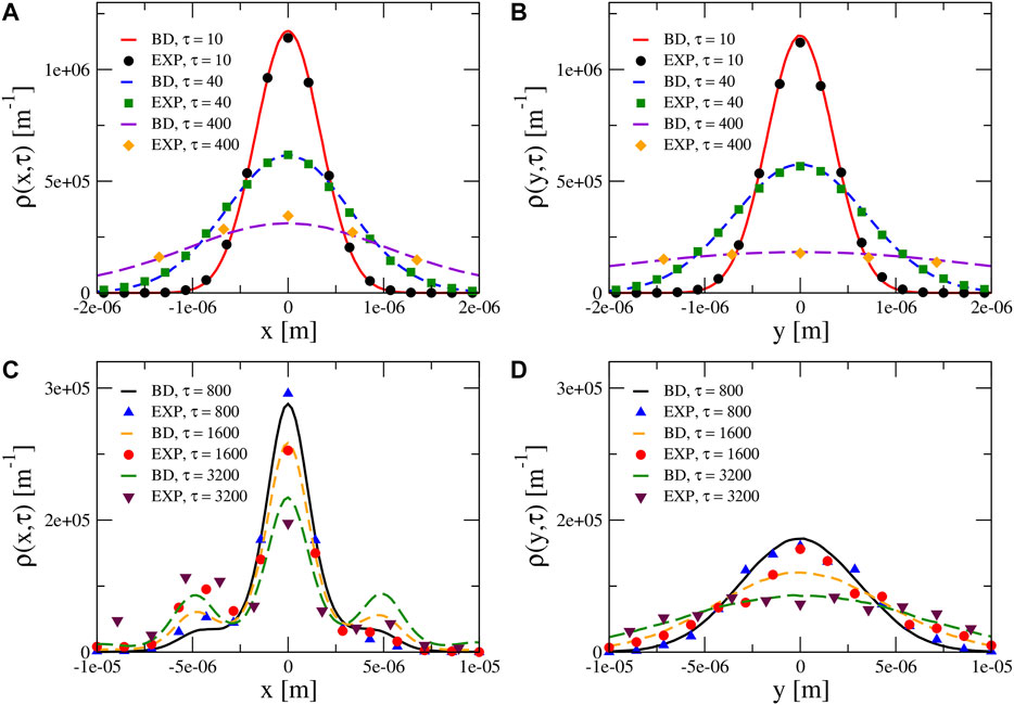
FIGURE 4. (Color online): Density of probability per unit length of finding a tracer $\rho \left(x,\tau \right)$ as a function of the position and the reduced time $\tau =t/\Delta t$, with $\Delta t=\left(1/30\right)s$. In panels (A,C) there is an applied periodic cosine-like external field in the x-axis direction. In panels (B,D) there is not an applied external field in the y-axis direction. Symbols correspond to experimental measurements. Lines are associated to Brownian dynamics simulations in which $D_0=1.8\times {10}^{-13}{m}^2/s$ and $U_0=1.33k_{B}T$.

In the absence of an external field, $\rho \left(x,t\right)$ displays a Gaussian behavior for all times displayed, as expected. Specifically, the maximum height $\rho \left(x=0,t\right)$ and the width of $\rho \left(x,t\right)$ decreases and increases, respectively, as a function of time. In the presence of a periodic external field, a similar behavior to that observed in the absence of an external field is seen only at very short times.

At longer times, the tracer starts to experience the external field and it is seen that: 1) the rate at which the maximum height $\rho \left(x,t\right)$ at x = 0 decreases becomes lower compared to the case in which the external field is not applied; and 2) the profile of $\rho \left(x,t\right)$ displays multiple damped maxima, which correspond to the spatial localization of the minima of the applied periodic external potential. This effect has been also reported in the literature [23]. A comparison of the rate at which the maximum of the density of probability $\rho \left(x,t\right)$ at x = 0 decreases, in the presence and in the absence of the periodic external field, is displayed in Figure 5 as function of time. Here, an excellent agreement is observed between experimental measurements and Brownian dynamics simulations.

FIGURE 5

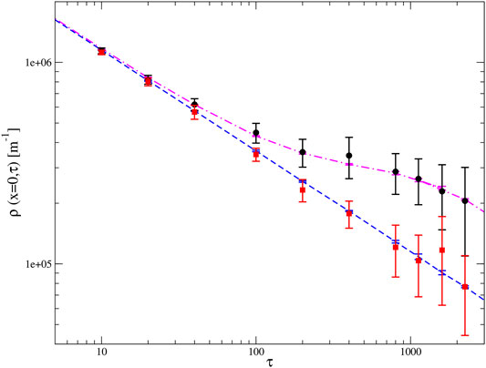
FIGURE 5. (Color online): Maximum of the density of probability of finding a tracer $\rho \left(x,\tau \right)$ at x = 0 as a function of the reduced time $\tau =t/\Delta t$, with $\Delta t=\left(1/30\right)s$. The solid squares and the dashed line correspond to experimental and Brownian dynamics results, respectively, in the absence of an external field. The black solid circles and the magenta dot-dashed line correspond to experimental and Brownian dynamics results, respectively, in the presence of a periodic cosine-like external field.

3.2 Mean Square Displacement and Long Time Dynamics

The good agreement observed between experimental and simulation results presented above, motivates a study of long time dynamic properties of the tracer via Brownian dynamics simulations for a fixed periodicity L. The MSD of a spherical tracer is displayed in Figure 6 as a function of time and the amplitude of the periodic potential $U_0$. Here, we observe that a change of curvature and a plateau appear, which is more noticeable when $U_0$ increases. As a whole, the behavior of the MSD found here is similar to reported results using simulations and experiments [23, 24]. Moreover, it is observed that the diffusion coefficient at long times, $D_M$, is significantly lower that the short time diffusion coefficient. $D_M$ and the Bellour parameters ${\delta }^2$ and α, were estimated by fitting the numerical results obtained from our Brownian dynamics simulations using the Bellour Eq. 5. These numerical values are displayed in Table 1. In contrast to the case in which tracer particles are dispersed in worm-like micelles solutions, with $\alpha \approx 0.25$, the α parameter here is higher than to 0.9, which gives a sharper transition between the short and the caging times regime. Interestingly, the asymptotic value of one is found in the solution to the Langevin equation for a parabolic potential [16]. The long time diffusion coefficient $D_M$ normalized with the short time diffusion coefficient $D_0$ is shown in Figure 7. In this figure, it is observed that $D_M/D_0$ decreases rapidly as a function of $U_0$, as expected from Figure 6, reaching a value close to $1\times {10}^{-5}$ for an energy barrier of $8k_{B}T$. In order to have a theoretical estimation of $D_M$ at long times, it is possible to use the Lifson-Jackson prescription (Eq. 15) or the Dalle-Ferrier et al. formula (Eq. 14) if the periodic potential is known. In this study, the periodic cosine potential given by Eq. 2 is fully defined in terms of the parameters $U_0$ and L. In Figure 7, it is observed that the Lifson-Jackson prescription provides an excellent estimation of the long time diffusion coefficient $D_M$ for all values of the maximum height of the periodic potential $U_0$ displayed. Contrastingly, the Dalle-Ferrier et al. approach shows a reasonable agreement, with the Brownian dynamics data, only for large values of $U_0$. In this regime, the Dalle-Ferrier et al. data tends to those yielded by the Lifson-Jackson prescription (see the inset of Figure 7).

FIGURE 6

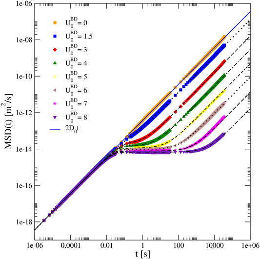
FIGURE 6. (Color online): Mean square displacement MSD(t) of a spherical tracer as a function of time in the presence of a periodic cosine-like potential of amplitude $U_0$. Solid symbols correspond to Brownian dynamics simulations in which $L=1.0\times {10}^{-6} m$ and $D_0^{BD}=D_0=1.8\times {10}^{-13} m^2/s$ for several $U_0^{BD}$ values (in $k_{B}T$ units). Dotted, dashed, and dot-dashed black lines correspond to Bellour fittings (Eq. 5) using the parameters displayed in Table 1.

TABLE 1

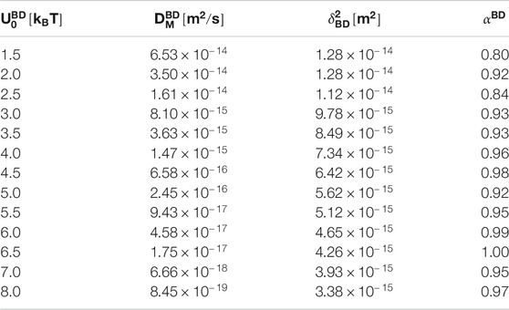
TABLE 1. Bellour fitting parameters $D_M^{BD}$, ${\delta }_{BD}^2$, and ${\alpha }^{BD}$ associated to the Brownian dynamics mean square displacement curves displayed in Figure 6, as a function of the maximum height barrier $U_0^{BD}$. In all Brownian dynamics simulations, $L=1.0\times {10}^{-6} m$ and $D_0^{BD}=D_0=1.8\times {10}^{-13} m^2/s$.

FIGURE 7

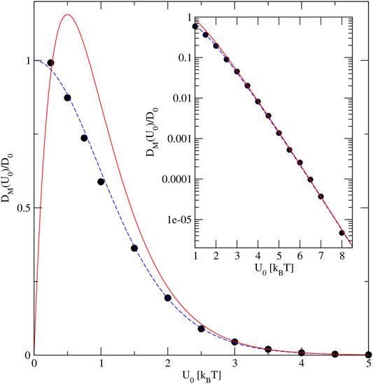
FIGURE 7. (Color online): Long-time diffusion coefficient $D_M\left(U_0\right)$ of a spherical tracer as a function of the maximum height barrier $U_0$. The black solid circles, the blue dashed-line, and the red solid-line correspond to Brownian dynamics, the Lifson-Jackson prescription (Eq. 15), and the Dalle-Ferrier formula (Eq. 14), respectively. In all cases, $L=1.0\times {10}^{-6} m$ and $D_0^{BD}=D_0=1.8\times {10}^{-13} m^2/s$.

In Figure 6 it appears that the time $t^{\text{*}}$ at which the first change of concavity of the MSD occurs is the same for all values of $U_0$ considered here. In order to locate this time more precisely, we calculate the logarithmic derivative of the MSD which is plotted in Figure 8 for different amplitudes of the periodic potential $U_0$. At very short and long times, the logarithmic derivative of the MSD tends to one, again showing a purely diffusive behavior. At intermediate values, the logarithmic derivative of the MSD shows a minimum at a time which we identify as $t^{\text{*}}$, i.e., at which a change of curvature of the MSD curve is observed. The magnitude of the logarithmic derivative at $t^{\text{*}}$ decreases as the energy barrier increases. Figure 9A shows the value of $t^{\text{*}}$as a function of $U_0$. Here it is observed that $t^{\text{*}}$ oscillates around the numerical value of 0.3 s. This suggests that the magnitude of $t^{\text{*}}$ is independent of the magnitude of $U_0$ for a fixed periodicity L. In the same figure, the value of the MSD at $t^{\text{*}}$ is shown, indicating a monotonic decrease by increasing $U_0$.

FIGURE 8

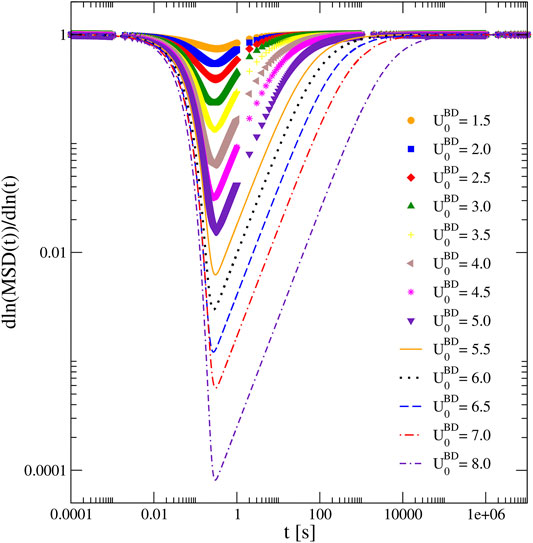
FIGURE 8. (Color online): Logarithmic derivative of the mean square displacement MSD(t) of a spherical tracer as a function of time in the presence of a periodic cosine-like potential of amplitude $U_0$. Solid symbols correspond to Brownian dynamics simulations in which $L=1.0\times {10}^{-6} m$ and $D_0^{BD}=D_0=1.8\times {10}^{-13} m^2/s$ for several $U_0^{BD}$ values (in $k_{B}T$ units).

FIGURE 9

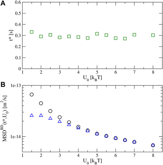
FIGURE 9. (Color online): (A) Critical time $t^{\ast }$ at which a change of curvature in the MSD is observed (green squares), and (B) mean square displacement at the critical time MSD ($t^{\text{*}}$) as a function of the maximum height barrier $U_0$ (black circles). The blue triangles are associated the Bellour fitting parameter $2{\delta }^{2BD}$ displayed in Table 1. These values were obtained from Brownian dynamics simulations in which $L=1.0\times {10}^{-6} m$ and $D_0=1.8\times {10}^{-13} m^2/s$ in all cases.

On the other hand, another interesting feature regarding the Bellour fitting is that the parameter $2{\delta }^{2BD}$ converge asymptotically to the MSD at the time $t^{\text{*}}$ for large $U_0$ values, as shown in Figure 9B. This gives a new interpretation of $2{\delta }^2$ in this type of periodical potentials.

The above mentioned effect related with the decrease of the $2{\delta }^{2BD}$ parameter increasing $U_0$, can be used to properly select the parameters for the random walker simulation. As a result, it is possible to compare the behavior of the random walker in the most simple periodic potential of periodic flat cages, to that displayed by a Brownian particle under the influence of a periodical potential as 2. If the cage-size and the transition probability p are chosen appropriately, this walker can also reproduce the same trend of the $D_M/D_0$ ratio as found in the BD simulation. As a consequence of the different potentials (a periodic cosine-like one vs. a flat cage with a delta barrier), the magnitude of the cage size decreases as p increases. Thus, the transition probability p is a monotonic decreasing function of the energy barrier. Interestingly, the MSD of the random walker is able to reproduce very accurately the MSD obtained from the BD simulations as shown in Figure 10, showing the same independence of $t^{\text{*}}$ for different transition probabilities (that are associated to different height barriers $U_0$). This suggests that the behavior of the particles in the two periodic potentials studied here would be the same in other periodic potentials.

FIGURE 10

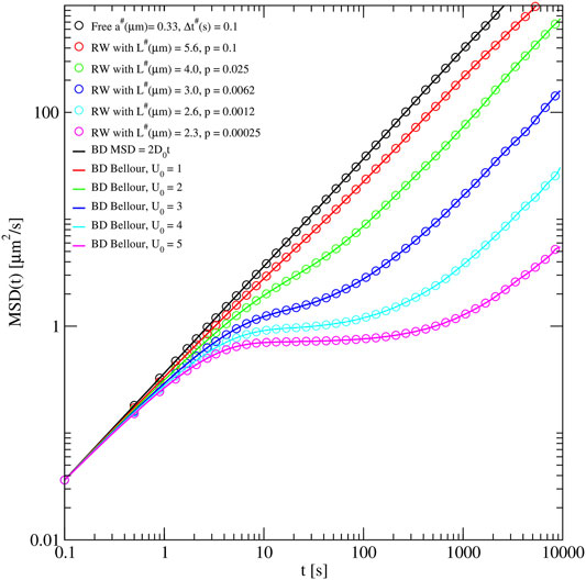
FIGURE 10. (Color online) Random walker MSD fitting of Brownian dynamics simulations in which the size of the periodic cell is $L=8$ microns for different energy barriers $U_0$ (in $K_{B}T$ units). The fitting parameters used in the random walker are the spatial and time increments $a^{\#}$ and $d{t}^{\#}$, which determine the short-times diffusion coefficient $D_0$; and the cage size $L^{\#}$ and the jump probability p, which determine the long-times diffusion coefficient $D_M$. These values are explicitly indicated in the labels.

3.3 Histograms of First Passage Time

In order to gain further insight about the independence of $t^{\text{*}}$ at different $U_0$ amplitudes of the periodic potential for a fixed periodicity L, in Figure 11 the histograms of the first passage time (FPT) τ of the tracer for several values of $U_0$ and different bin values are displayed. In all analyzed cases, it is observed that short FTPs are very rare events, giving also a measure of the time required for the particles to reach the barrier by Brownian motion. When the magnitude of the FTP increases, its frequency of occurrence increases too. This augment of the frequency of occurrence of the escape time is observed until a critical value $t^{\prime }$ is reached. At the critical FPT $t^{\prime }$ the histogram displays a maximum. The time $t^{\prime }$ is then the most likely FPT of the tracer. For larger FPTs, the associated frequency of occurrence decreases exponentially. Thus, the tail of each FPT histogram (for FPTs larger than $t^{\prime }$) is fitted to a simple exponential of the form:

$F\left(\tau \right)=A\exp \left(-K\tau \right)(20)$

where F is the frequency of events in the escape time histogram, A is the asymptotic value of F when $\tau =0$, and K is the decay constant of the escape times. These three quantities depend on the selected values of the bin of the histogram, $D_0$, $U_0$, and L. In each panel of Figure 11, $D_0$, $U_0$, and L are kept constant, and different histograms are displayed as a function of the value of the bin used.

FIGURE 11

FIGURE 11. (Color online):Brownian dynamics histograms of the first passage time (FPT) τ for different barrier heights $U_0$ and $\text{Δ}t$ bins. The value of $U_0$ in $k_{B}T$ units is 1, 2, 3, and 4 for (A–D), respectively. The $\Delta t$ bin is 0.08, 0.04, 0.02, and 0.01 s for pink circles, red squares, blue diamonds, and green triangles, respectively. Black lines are exponential tail fittings associated to Eq. 20. For a given $U_0$ value, the vertical purple solid line corresponds to the critical time $t^{\text{*}}$, and the vertical orange dashed line indicates the mean first passage time ${\tau }_{MFPT}$. The periodicity of the fringe and the short times diffusion coefficient are $L=1.0\times {10}^{-6} m$ and $D_0^{BD}=D_0=1.8\times {10}^{-13} m^2/s$, respectively, in the Brownian dynamics simulations.

On the other hand, all histograms displayed in Figure 11 are normalized dividing the value of F by the corresponding value of A, that is:

$F^{\ast }\left(\tau \right)=F\left(\tau \right)/A(21)$

These normalized histograms are shown in Figure 12. Here, we observe that all normalized MFPT histograms collapse onto the same curve for different bin values. Moreover, it is observed that the most likely FPT $t^{\prime }$ (that is, the FTP at which a maximum is observed in each histogram) displays approximately a constant value independently of the height of the periodic potential $U_0$. In addition, the magnitude of $t^{\prime }$ is very close to the magnitude of $t^{\text{*}}$. As a result, the change of curvature observed in the MSD at $t^{\text{*}}$ can be physically related to the characteristic time at which the MFPT starts to display its more likely value. Contrastingly, the mean first passage time (MFPT) ${\tau }_{MFPT}$ strongly depends on the value of the height barrier $U_0$ as it is shown in Figure 13. The escape time ${\tau }_{escape}=2{\tau }_{MFPT}$ obtained from the Brownian dynamics simulations are displayed in Figure 13 as a function of the height barrier $U_0$. The theoretical values predicted by Eqs 16, 17 corresponding to the Dale-Ferrier and the Lifson-Jackson approaches, respectively, are also shown. The Dale-Ferrier formula break downs at low height barriers $U_0$, whereas the Lifson-Jackson Eq. predicts the expected limit ${\tau }_{escape}={\tau }_0$, where ${\tau }_0=\frac{L^2}{2D_0}$. In both theoretical approaches, the escape time ${\tau }_{escape}$ increases exponentially as a function of the height barrier $U_0$ and both descriptions converge to the same value at height barriers. For all displayed values, the escape time ${\tau }_{escape}$ produced by the Lifson-Jackson equation displays an excellent agreement with the data obtained from the Brownian dynamics simulations. On the other hand, it is interesting to note that the histograms of the FTP displayed in Figure 12 resemble the distribution of first passage times in complex geometries [46–49], or in energy landscapes [50–53], and are actually closely related. Here, we focus the discussion on the relationship between the histograms of escape times and a more simple statistical quantity such as the MSD.

FIGURE 12

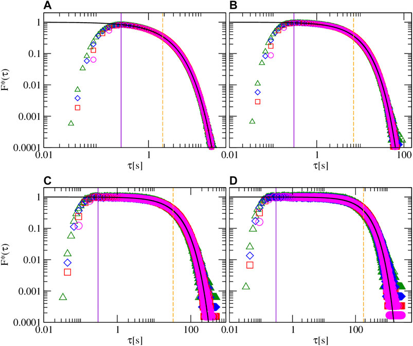
FIGURE 12. (Color online): Normalized histograms of the first passage times for different barrier heights $U_0$ and $\text{Δ}t$ bins. Black lines are exponential tail fittings associated to Eq. 21. Locants have the same meaning as that used in Figure 11.

FIGURE 13

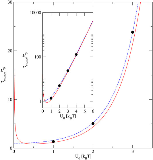
FIGURE 13. (Color online): Escape time ${\tau }_{escape}=2{\tau }_{MFPT}$ as a function of the barrier height $U_0$. The black solid circles, the blue dashed-line and the red solid line have been obtained from Brownian dynamics, the Lifson-Jackson prescription (Eq. 17), and the Dalle-Ferrier formula (Eq. 16), respectively. In all cases, ${\tau }_0=\frac{L^2}{2D_0}$, $L=1.0\times {10}^{-6} m$ and $D_0^{BD}=D_0=1.8\times {10}^{-13} m^2/s$.

As pointed out above, important features of the motion of a colloidal particle in a periodic potential are also presented in the simple model of a random walker. Another interesting quantity is the escape time whose histograms for the random walker simulation were also calculated and shown in Figure 14. The normalization of the histograms were performed following the same protocol used in the BD simulations. Here, it can be observed a behavior analogous to that observed by BD simulations: the frequency of short escape times increases as the escape time increases. This augment of the frequency of occurrence of the escape time is observed until a critical value $t^{\prime }$ is reached. At the critical escape time $t^{\prime }$ the histogram displays a maximum. The time $t^{\prime }$ is then the most likely escape time of the tracer. For larger escape times, the associated frequency of occurrence decreases exponentially.

FIGURE 14

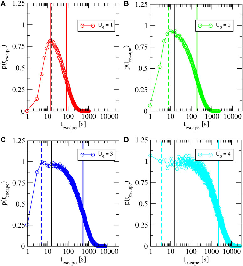
FIGURE 14. (Color online) Normalized histograms of the escape times obtained from the random walker simulations. The data are labeled according to the target Brownian dynamics simulations displayed in Figure 10. Vertical blue, green, and red dashed lines represent the mean time $t^{\#}$ required by the random walker to reach one boundary of a periodic cell of size $L^{\#}$, given that the random walk started at any point inside the periodic cell. Vertical blue, green, and red continuous solid lines are associated to the mean value of the escape time in the random walker model. The vertical black continuous solid line indicates the average critical time $t^{\text{*}}$ obtained from the Brownian dynamics data.

Let us define now $t^{\#}$ as the mean time required by the walker to reach the boundary of the cell, given that it started at any point of the cell of length $L^{\#}$. This time is displayed by vertical colored-dashed lines in Figure 14 for several transition probabilities, which can be associated to the $U_0$ barrier heights used in the BD simulations. In this figure, it is observed that the time $t^{\#}$ is located very close to the more likely escape time $t^{\prime }$, which is equal to 15, 17, 17, and 25 s for $U_0$ equal to 1, 2, 3, and 4 k_BT, respectively. Thus, it is possible to interpret the more likely escape time as the mean time $t^{\#}$ required by the walker to reach one of the boundary of the cells given that started at any point of a cell of length $L^{\#}$. As this time depends mainly on $L^{\#}$ and not on p, and $L^{\#}$ is of the same order of magnitude for the different $U_0$ values, all $t^{\#}$ times are located close among them. Moreover, it is observed that all $t^{\#}$ times are close to the average time $t^{\text{*}}$ of the BD simulations. Then, it is possible to propose that the characteristic times $t^{\prime }$ and $t^{\#}$ can be approximated by $t^{\text{*}}$, which can be easily measured from MSD curves. Notice that the mean value of the escape time, displayed as a vertical colored-solid line, strongly depends on the $U_0$ value. The above mentioned results can be summarized following the next arguments and considering the ensemble of particles located in the periodic potential and undergoing Brownian motion: at long escape times, longer than $t^{\#}$ the escape process can be considered stationary: considering a time window of constant width, at each time window a fraction of the remaining particles are escaping from the potential, giving an exponential decay of the histograms of escape times. Such fraction decreases as $U_0$ increases. The absence of escape events at very short times, and the further increase is related with an increase in the number of particles reaching the barrier for the first time. This first regime is mostly independent on the energy barrier and dominated by the periodicity of the potential. The independence of the most likely time $t^{\prime }$ on the energy barrier $U_0$ is related to the onset of the stationary regime at long times. Thus, the time at which the MSD reaches the plateau and starts to develop the second diffusive regime, characterized by the parameter $t^{\ast }$, can be used to differentiate the short- and long-time regimes that the spherical tracer experiences under the influence of a periodic external field, in terms of the behavior of the escape time histograms.

4 Conclusion

In this work, we have studied some dynamic properties of a Brownian tracer in two periodic potentials at short- and long-times. For the experimentally obtained harmonic potential, at short-times, the proposed protocol allowed us to estimate the short time diffusion coefficient $D_0$ and the maximum height of the potential $U_0$, by performing a numerical fitting of the MSD of the tracer obtained via experiments and Brownian dynamics simulations. The precision of these parameters was further tested by calculating another microscopic time dependent property, namely, the linear density of probability per unit length of finding the tracer at a position x at a time t. At long-times, Brownian dynamics simulations were performed to study some dynamic properties of the tracer such as the MSD. The numerical MSDs obtained via Brownian dynamics were also fitted to the Bellour equation. Using the parameters found, a simpler random walker simulation was also performed in order to test our results in one of the most simple forms of a periodic potential.

At the level of the MSD, it was observed that a plateau and a change of curvature appear and become more conspicuous when the $U_0$ increases. The long time diffusion coefficient of the tracer $D_M$, obtained from the Brownian dynamics simulations, decreased rapidly as a function of $U_0$ for a fixed periodicity L. In order to estimate $D_M$ from first principles, we used the Lifson-Jackson prescription and the analytic Dalle-Ferrier et al. formula. An excellent agreement between the long time $D_M$ of the tracer obtained via the Lifson-Jackson prescription and the corresponding Brownian dynamics simulations is observed. On the other hand, the Dalle-Ferrier et al. formula produces long time $D_M$ coefficients that converge asymptotically, at large $U_0$ values, to those predicted by our simulations and the Lifson-Jackson approach. By selecting properly the random walker simulation parameters, the same trend of the long time diffusion coefficient is obtained.

In order to locate clearly the time $t^{\text{*}}$ at which a plateau and the first change of curvature appear at large values of $U_0$, the logarithmic derivative of the MSD was calculated for different values of $U_0$. It is found that the magnitude of $t^{\text{*}}$ remains approximately constant and independent of $U_0$ for a fixed periodicity L of the periodic potential, finding the same results for the case of the periodic potential associated to the random walker by increasing the probability of hopping p. The most likely escape time $t^{\prime }$ of the tracer displays an analogous behavior regarding $U_0$ or p, and the magnitude of $t^{\prime }$ is very similar to the magnitude of $t^{\text{*}}$. Thus, the change of curvature observed in the MSD at $t^{\text{*}}$ can be physically related to the characteristic time at which the escape time starts to display its more likely value. Moreover, the critical time $t^{\text{*}}$ obtained from a single MSD curve can be used as a first approximation of the most likely escape time $t^{\prime }$, obtained from computationally expensive escape time histograms.

The two periodic potentials studied here via experiments, Brownian dynamics, and random walker simulations constitute very simple models useful to characterize or describe more complex systems such as dense polyelectrolyte solutions, jammed spheres, and even crowded biological structures as those found inside living cells. In this sense, if our simple models are able to provide the long time diffusion coefficient $D_M$ of a tracer in a dense and crowded experimental environment, then the associated maximum height and periodicity of the cosine potential can be used as effective parameters describing the characteristic energy barrier that the tracer needs to overcome in order to jump, or escape, from one effective confining cell to another one. The application of this approach to characterize the long time dynamics of a tracer in dense tubular micellar solutions is in progress and will be published elsewhere.

Data Availability Statement

The raw data supporting the conclusions of this article will be made available by the authors, without undue reservation.

Author Contributions

ES-G and JA-L designed the experiments. ES-G and DP-G implemented the experimental set-up. DP-G performed the experiments. GG-G and DP-G implemented the BD simulations. ES-G designed and implemented the random walker simulation. GG-G, DP-G, JA-L and ES-G analyzed the data. GG-G, DP-G, JA-L and ES-G wrote the manuscript.

Funding

GG-G acknowledges the Marcos Moshinsky Fellowship, the SEP-CONACYT CB-2016 grant 286105, the PRODEP grant UASLP-PTC-652 511-6/2020-8585, the CONACYT grants 261210 and FC-2015-2-1155, and the Laboratorio Nacional de Ingeniería de la Materia Fuera de Equilibrio-279887-2017 for the financial funding. ES-G acknowledges CONACYT Mexico through grant A1-S-9098. Authors thanks Prof. Stefan Egelhaaf for useful discussions.

Conflict of Interest

The authors declare that the research was conducted in the absence of any commercial or financial relationship that could be construed as a potential conflict of interest.

Acknowledgments

The authors thankfully acknowledge computer resources, technical advice and support provided by the Laboratorio Nacional de Supercómputo del Sureste de México (LNS), a member of the CONACYT national laboratories, with project No. 202001024N; as well as the Centro Nacional of Supercómputo (CNS) for the computing time provided at THUBAT KAAL II. GG-G. expresses his gratitude for the assistance from the computer technicians at the IF-UASLP.

5 Appendix

As both the Dalle-Ferrier et al. formula, and the Bellour fitting parameter $2{\delta }^{2BD}$ converge asymptotically to the Lifson-Jackson prescription, and the MSD at the time $t^{\text{*}}$, respectively, for large $U_0$ values, the associated errors are displayed in Figures 15A,B. In Figure 15, it is observed that the error of the Dalle-Ferrier et al. analytic formula is of the order of ten percent for $U_0=3K_{B}T$. This error can be decreased by increasing the magnitude of $U_0$. However, the error cannot be reduced less than 2 percent even for maximum heights of the periodic potential as large as $U_0=10$$K_{B}T$. On the other hand, the error in the convergence of the Bellour fitting parameter $2{\delta }^{2BD}$ regarding the MSD at the time $t^{\text{*}}$ is similar to that displayed by the Dalle-Ferrier et al. formula at $U_0=3K_{B}T$, even though it reduces very quickly becoming as small as 0.01 percent for $U_0=3K_{B}T$.

FIGURE 15

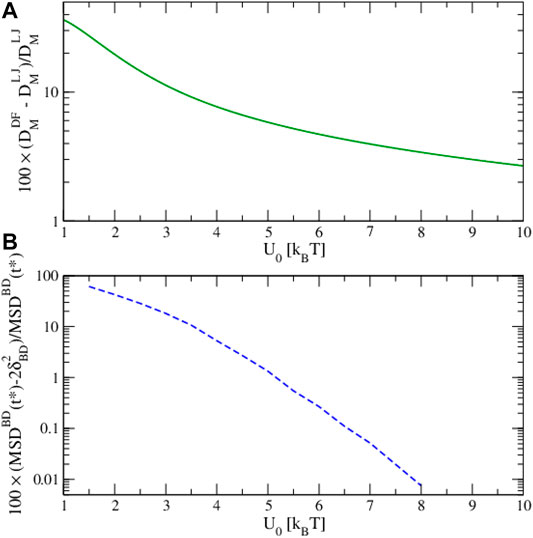
FIGURE 15. (Color online): (A) Error of the long-time diffusion coefficient obtained from the Dalle-Ferrier formula $D_M^{DF}$ regarding the value predicted by the Lifson-Jackson $D_M^{LJ}$ prescription, and (B) difference between the fitting Bellour parameter $2{\delta }^2$ and the mean square displacement at the critical time $MSD\left(t^{\ast }\right)$ as a function of the maximum height barrier $U_0$. These results were obtained from Brownian dynamics simulations in which $L=1.0\times {10}^{-6} m$ and $D_0=1.8\times {10}^{-13} m^2/s$ in all cases.

References

1. Golding I, Cox EC. Physical nature of bacterial cytoplasm. PRL (2006) 96:098102. doi:10.1103/physrevlett.96.098102

CrossRef Full Text | Google Scholar

2. Tolić-Nørrelykke IM, Munteanu EL, Thon G, Oddershede L, Berg-Sørensen K. Anomalous diffusion in living yeast cells. Phys Rev Lett (2004) 93:078102. doi:10.1103/PhysRevLett.93.078102

PubMed Abstract | CrossRef Full Text | Google Scholar

3. Weiss M, Elsner M, Kartberg F, Nilsson T. Anomalous subdiffusion is a measure for cytoplasmic crowding in living cells. Biophys J (2004) 87:3518–24. doi:10.1529/biophysj.104.044263

PubMed Abstract | CrossRef Full Text | Google Scholar

4. Xia Q, Xiao H, Pan Y, Wang L. Microrheology, advances in methods and insights. Adv Coll Int Sci (2018) 257:71–85. doi:10.1016/j.cis.2018.04.008

CrossRef Full Text | Google Scholar

5. Sarmiento-Gomez E, Lopez-Diaz D, Castillo R. Microrheology and characteristic lengths in wormlike micelles made of a zwitterionic surfactant and sds in brine. J Phys Chem B (2010) 114:12193–202. doi:10.1021/jp104996h

PubMed Abstract | CrossRef Full Text | Google Scholar

6. Mason TG, Weitz DA. Optical measurements of frequency-dependent linear viscoelastic moduli of complex fluids. Phys Rev Lett (1995) 74:1250–3. doi:10.1103/physrevlett.74.1250

PubMed Abstract | CrossRef Full Text | Google Scholar

7. Schnurr B, Gittes F, MacKintosh FC, Schmidt CF. Determining microscopic viscoelasticity in flexible and semiflexible polymer networks from thermal fluctuations. Macromolecules (1997) 30:7781–92. doi:10.1021/ma970555n

CrossRef Full Text | Google Scholar

8. Amblard F, Maggs AC, Yurke B, Pargellis A, Leibler S. Subdiffusion and anomalous local viscoelasticity in actin networks. Phys Rev Lett (1999) 77:4470. doi:10.1103/PhysRevLett.77.4470

CrossRef Full Text | Google Scholar

9. Bellour M, Skouri M, Munch JP, Hébraud P. Brownian motion of particles embedded in a solution of giant micelles. Eur Phys J E (2002) 8:431–6. doi:10.1140/epje/i2002-10026-0

PubMed Abstract | CrossRef Full Text | Google Scholar

10. Hunter GL, Weeks ER. The physics of the colloidal glass transition. Rep Prog Phys (2012) 75:066501. doi:10.1088/0034-4885/75/6/066501

PubMed Abstract | CrossRef Full Text | Google Scholar

11. Weeks ER. Introduction to the colloidal glass transition. ACS Macro Lett (2017) 6:27–34. doi:10.1021/acsmacrolett.6b00826

CrossRef Full Text | Google Scholar

12. Löwen H. Colloidal dispersions in external fields: recent developments. J Phys Condens Matter (2008) 20:404201. doi:10.1088/0953-8984/20/40/404201

CrossRef Full Text | Google Scholar

13. Zhu J, Li M, Rogers R, Meyer W, Ottewill RH, Russel WB, et al. Crystallization of hard-sphere colloids in microgravity. Nature (1997) 387:883–5. doi:10.1038/43141

CrossRef Full Text | Google Scholar

14. Sprenger HJ, Marquardt P, Tadros TF. The scope of microgravity experiments in colloid science: major conclusions from the workshop. Adv Coll Int Sci (1993) 46:343–7. doi:10.1016/0001-8686(93)80048-g

CrossRef Full Text | Google Scholar

15. Bailey AE, Poon WCK, Christianson RJ, Schofield AB, Gasser U, Prasad V, et al. Spinodal decomposition in a model colloid-polymer mixture in microgravity. Phys Rev Lett (2007) 99:205701. doi:10.1103/physrevlett.99.205701

PubMed Abstract | CrossRef Full Text | Google Scholar

16. Pesce G, Volpe G, Maragó OM, Jones PH, Gigan S, Sasso A, et al. Step-by-step guide to the realization of advanced optical tweezers. J Opt Soc Am B (2015) 32:B84–98. doi:10.1364/josab.32.000b84

CrossRef Full Text | Google Scholar

17. Evers F, Hanes RDL, Zunke C, Capellmann RF, Bewerunge J, Dalle-Ferrier C, et al. Colloids in light fields: particle dynamics in random and periodic energy landscapes. Eur Phys J Spec Top (2013) 222:2995–3009. doi:10.1140/epjst/e2013-02071-2

CrossRef Full Text | Google Scholar

18. Romero AH, Sancho JM. Brownian motion in short range random potentials. Phys Rev E (1998) 58:2833–7. doi:10.1103/physreve.58.2833

CrossRef Full Text | Google Scholar

19. Sancho JM, Lacasta AM, Lindenberg K, Sokolov IM, Romero AH. Diffusion on a solid surface: anomalous is normal. Phys Rev Lett (2004) 92:250601. doi:10.1103/physrevlett.92.250601

PubMed Abstract | CrossRef Full Text | Google Scholar

20. Schmiedeberg M, Roth J, Stark H. Brownian particles in random and quasicrystalline potentials: how they approach the equilibrium. Eur Phys J E Soft Matter (2007) 24:367–77. doi:10.1140/epje/i2007-10247-7

PubMed Abstract | CrossRef Full Text | Google Scholar

21. Hanes RDL, Schmiedeberg M, Egelhaaf SU. Brownian particles on rough substrates: relation between intermediate subdiffusion and asymptotic long-time diffusion. Phys Rev Lett (2013) 88:062133. doi:10.1103/physreve.88.062133

CrossRef Full Text | Google Scholar

22. Furst EM, Squires TM. Microrheology. New York, NY: Oxford University Press (2017).

23. Dalle-Ferrier C, Krüger M, Hanes RDL, Walta S, Jenkins MC, Egelhaaf SU. Dynamics of dilute colloidal suspensions in modulated potentials. Soft Matter (2011) 7:2064–75. doi:10.1039/c0sm01051k

CrossRef Full Text | Google Scholar

24. Velarde SH, Castaneda-Priego R. Diffusion in two-dimensional colloidal systems on periodic substrates. Phys Rev E (2009) 79:041407. doi:10.1103/PhysRevE.79.041407

CrossRef Full Text | Google Scholar

25. Wei QH, Bechinger C, Rudhardt D, Leiderer P. Experimental study of laser-induced melting in two-dimensional colloids. Phys Rev Lett (1998) 81:2606. doi:10.1103/physrevlett.81.2606

CrossRef Full Text | Google Scholar

26. Capellmann RF, Bewerunge J, Platten F, Egelhaaf SU. Note: using a Kösters prism to create a fringe pattern. Rev Scientific Instr (2017) 88:056102. doi:10.1063/1.4982587

CrossRef Full Text | Google Scholar

27. Metzler R, Jeon JH, Cherstvy AG, Barkai E. Anomalous diffusion models and their properties: non-stationarity, non-ergodicity, and ageing at the centenary of single particle tracking. Phys Chem Chem Phys (2014) 16:24128–64. doi:10.1039/c4cp03465a

PubMed Abstract | CrossRef Full Text | Google Scholar

28. Metzler R, Klafter J. The random walk’s guide to anomalous diffusion: a fractional dynamics approach. Phys Rep (2000) 339:1–77. doi:10.1016/s0370-1573(00)00070-3

CrossRef Full Text | Google Scholar

29. Muñoz-Gil G, Garcia-March MA, Manzo C, Celi A, Lewenstein M. Diffusion through a network of compartments separated by partially-transmitting boundaries. Front Phys (2019) 7:31. doi:10.3389/fphy.2019.00031

CrossRef Full Text | Google Scholar

30. Lifson S, Jackson JL. On the self-diffusion of ions in a polyelectrolyte solution. J Chem Phys (1962) 36:2410–4. doi:10.1063/1.1732899

CrossRef Full Text | Google Scholar

31. Hänggi P, Talkner P, Borkovec M. Reaction-rate theory: fifty years after kramers. Rev Mod Phys (1990) 62:251–341. doi:10.1103/revmodphys.62.251

CrossRef Full Text | Google Scholar

32. Megen WV, Underwood SM. The glass transition in colloidal hard spheres. J Phys Condens Matter (1994) 6:A181–186. doi:10.1088/0953-8984/6/23a/026

CrossRef Full Text | Google Scholar

33. Carvajal-Tinoco MD, de León GC, Arauz-Lara JL. Brownian motion in quasibidimensional colloidal suspensions. Phys Rev E (1997) 56:6962–9. doi:10.1103/PhysRevE.56.6962

CrossRef Full Text | Google Scholar

34. Sarmiento-Gómez E, Rivera-Morán JA, Arauz-Lara JL. Energy landscape of colloidal dumbbells in a periodic distribution of light. Soft Matter (2019) 15:3573–9. doi:10.1039/c9sm00472f

PubMed Abstract | CrossRef Full Text | Google Scholar

35. Jenkins MC, Egelhaaf SU. Colloidal suspensions in modulated light fields. J Phys Condens Matter (2008) 20:404220. doi:10.1088/0953-8984/20/40/404220

CrossRef Full Text | Google Scholar

36. Ashkin A. Forces of a single-beam gradient laser trap on a dielectric sphere in the ray optics regime. Biophys J (1992) 61:569–82. doi:10.1016/s0006-3495(92)81860-x

PubMed Abstract | CrossRef Full Text | Google Scholar

37. Harada Y, Asakura T. Radiation forces on a dielectric sphere in the Rayleigh scattering regime. Opt Commun (1996) 124:529–41. doi:10.1016/0030-4018(95)00753-9

CrossRef Full Text | Google Scholar

38. Allan DB, Caswell TA, Keim NC. trackpy: Trackpy v0.3.2 (Version v0.3.2). Zenodo (2019). doi:10.5281/zenodo.60550

39. Crocker JC, Grier DG. Methods of digital video microscopy for colloidal studies. J Colloid Interf Sci (1996) 179:298–310. doi:10.1006/jcis.1996.0217

CrossRef Full Text | Google Scholar

40. Ermak DL. A computer simulation of charged particles in solution. i. technique and equilibrium properties. J Chem Phys (1975) 62:4189–96. doi:10.1063/1.430300

CrossRef Full Text | Google Scholar

41. Pérez-Guerrero D. Statistical transitions of colloidal particles into two-dimensional periodic external potentials (in Spanish). [Bachelor’s thesis]. San Luis (México): Facultad de Ciencias de la Universidad Autónoma de San Luis Potosí (2018).

42. Ferrando R, Spadacini R, Tommei GE. Kramers problem in periodic potentials: jump rate and jump lengths. Phys Rev E (1993) 48:2437–51. doi:10.1103/physreve.48.2437

CrossRef Full Text | Google Scholar

43. Pavliotis GA, Vogiannou A. Diffusive transport in periodic potentials: underdamped dynamics. Fluct Noise Lett (2008) 08:L155–L173. doi:10.1142/s0219477508004453

CrossRef Full Text | Google Scholar

44. McLeish TCB. Thermal barrier hopping in biological Physics. Boca Raton, Florida: CRC Press (2006). p. 123–35.

CrossRef Full Text

45. Sarmiento-Gómez E, Villanueva-Valencia JR, Herrera-Velarde S, Ruiz-Santoyo JA, Santana-Solano J, Arauz-Lara JL, et al. Short-time dynamics of monomers and dimers in quasi-two-dimensional colloidal mixtures. Phys Rev E (2016) 94:012608. doi:10.1103/physreve.94.012608

PubMed Abstract | CrossRef Full Text | Google Scholar

46. Rupprecht JF, Bénichou O, Grebenkov DS, Voituriez R. Exit time distribution in spherically symmetric two-dimensional domains. J Stat Phys (2014) 158:192–230. doi:10.1007/s10955-014-1116-6

CrossRef Full Text | Google Scholar

47. Mattos TG, Carlos MM, Metzler R, Oshanin G. First passages in bounded domains: when is the mean first passage time meaningful?. Phys Rev E (2012) 86:031143. doi:10.1103/physreve.86.031143

CrossRef Full Text | Google Scholar

48. Singer A, Schuss Z, Holcman D. Narrow escape, part iii: non-smooth domains and riemann surfaces. J Stat Phys (2006) 122:491–509. doi:10.1007/s10955-005-8028-4

CrossRef Full Text | Google Scholar

49. Mejía-Monasterio C, Oshanin G, Schehr G. First passages for a search by a swarm of independent random searchers. J Stat Mech Theor Exp (2011) 2011:P06022. doi:10.1088/1742-5468/2011/06/p06022

CrossRef Full Text | Google Scholar

50. Chupeau M, Gladrow J, Chepelianskii A, Keyser UF, Trizac E. Optimizing brownian escape rates by potential shaping. Proc Natl Acad Sci (2020) 117:1383–8. doi:10.1073/pnas.1910677116

PubMed Abstract | CrossRef Full Text | Google Scholar

51. Coughlan ACH, Torres-Díaz I, Zhang J, Bevan MA. Non-equilibrium steady-state colloidal assembly dynamics. J Chem Phys (2019) 150:204902. doi:10.1063/1.5094554

PubMed Abstract | CrossRef Full Text | Google Scholar

52. Edwards T, Yang Y, Beltran-Villegas D, Bevan M. Colloidal crystal grain boundary formation and motion. Scientific Rep (2014) 4:6132. doi:10.1038/srep06132

CrossRef Full Text | Google Scholar

53. Palyulin VV, Metzler R. How a finite potential barrier decreases the mean first-passage time. J Stat Mech Theor Exp (2012) 2012:L03001. doi:10.1088/1742-5468/2012/03/l03001

CrossRef Full Text | Google Scholar