Rogue Waves With Rational Profiles in Unstable Condensate and Its Solitonic Model

In this brief report we study numerically the spontaneous emergence of rogue waves in 1) modulationally unstable plane wave at its long-time statistically stationary state and 2) bound-state multi-soliton solutions representing the solitonic model of this state. Focusing our analysis on the cohort of the largest rogue waves, we find their practically identical dynamical and statistical properties for both systems, that strongly suggests that the main mechanism of rogue wave formation for the modulational instability case is multi-soliton interaction. Additionally, we demonstrate that most of the largest rogue waves are very well approximated–simultaneously in space and in time–by the amplitude-scaled rational breather solution of the second order.

1 Introduction

The phenomenon of rogue waves (RWs)—unusually large waves that appear suddenly from moderate wave background–was intensively studied in the recent years. A number of mechanisms were suggested to explain their emergence, see e.g., the reviews [1–3]; with the most general idea stating that RWs could be related to breather-type solutions of the underlying nonlinear evolution equations [4–6]. Currently, ones of the most popular models for RWs are the Peregrine rational breather [7] and the higher-order rational breather [8] solutions of the one-dimensional nonlinear Schrödinger equation (1D-NLSE) of the focusing type,

$i{\psi }_t+{\psi }_{xx}+{\left|\psi \right|}^2\psi =0(1)$

These solutions belong to a family of localized in space and time algebraic breathers, which evolve on a finite background and lead to three-fold, five-fold, seven-fold, and so on, increase in amplitude at the time of their maximum elevation. Taking specific and carefully designed initial conditions, they were reproduced in well-controlled experiments performed in different physical systems [9–13].

The 1D-NLSE is integrable in terms of the inverse scattering transform (IST), as it allows transformation to the so-called scattering data, which is in one-to-one correspondence with the wavefield and, similarly to the Fourier harmonics in the linear wave theory, changes trivially during the motion. Thanks to its properties, the scattering data can be used to characterize the wavefield. For spatially localized case, the scattering data consists of the discrete (solitons) and the continuous (nonlinear dispersive waves) parts of eigenvalue spectrum, calculated for specific auxiliary linear system. For strongly nonlinear wavefields, such as the ones where emergence of rational breathers can be expected, the solitons provide the main contribution to the energy [14] and should therefore play the dominant role in the dynamics. In particular, as has been recently demonstrated in [15]; the modulationally unstable plane wave (the condensate) at its long-time statistically stationary state can be accurately modeled (in the statistical sense) with a certain soliton gas, designed to follow the solitonic structure of the condensate. The latter naturally raises a question of whether there is a difference between the RWs emerging in the two systems. Indeed, in a soliton gas all RWs are multi-soliton interactions by construction. Hence, if there is no significant difference, then we can draw a hypothesis that for the asymptotic stationary state of the MI (and, possibly, for other strongly nonlinear wavefields) the main mechanism of RW formation is interaction of solitons.

With the present paper, we contribute to the answer on this question by summarizing our observations of RWs for both systems. Specifically, we compute time evolution for 1,000 random realizations of the noise-induced MI of the condensate and also for 1,000 random realizations of 128-soliton solutions modeling the asymptotic state of the MI. For each realization, we analyze one largest RW emerging in the course of the evolution, thus focusing our analysis on the largest RWs. For both systems, we observe practically identical dynamical and statistical properties of the collected RWs. In particular, most of the RWs turn out to be very well approximated–simultaneously in space and in time–by the amplitude-scaled rational breather solution (RBS) of the second order. By measuring deviation between RWs and their fits with RBS as an integral of the difference in the $\left(x,t\right)$-space, we find that, in general, the larger the maximum amplitude of the RW, the better its convergence to the RBS of the second order (RBS2). The collected RWs for the two systems turn out to be identically distributed by their maximum amplitude and deviation from the RBS2. Additionally, we demonstrate that the observed quasi-rational profiles appear already for synchronized three-soliton interactions and discuss the next steps in the ongoing research of the RW origin.

Note that in the present paper we consider solutions of the 1D-NLSE for three different types of boundary conditions: the MI of the condensate for which we use the periodic boundary, the multi-soliton solutions with vanishing border conditions and the RBS having constant border conditions at infinity. Globally, these solutions are fundamentally different, and the different border conditions require application of separate IST techniques, see e.g., [5, 14, 16, 17]. For instance, formally our MI case corresponds to finite-band scattering data. However, the characteristic widths of the structures (RWs, solitons, RBS) are small compared to the sizes of the studied wavefields, so that the eigenvalue bands are very narrow and we neglect their difference from solitons. The similar idea was suggested in [18]; where, vice versa, the soliton gas was considered as a limit of finite-band solutions. Effectively, we assume that formation of a RW, as a local phenomenon, represents a similar process for all three cases of border conditions. As we demonstrate in the paper, this assumption is supported by the presented results, that raises an important problem that we leave for future studies–explanation of how the three models may exhibit locally similar nonlinear patterns.

2 Numerical Methods

For both the MI of the condensate and the soliton gas initial conditions, we solve Eq. 1 numerically in a large box $x\in \left[-L/2,L/2\right]$, $L\gg 1$, with periodic boundary. We use the pseudo-spectral Runge-Kutta fourth-order method in adaptive grid with the grid size $\Delta x$ set from the analysis of the Fourier spectrum of the solution; see [19] for detail. As an integrable equation, the 1D-NLSE conserves an infinite set of integrals of motion, see e.g., [14]. We have checked that the first ten integrals are conserved by our numerical scheme up to the relative errors from ${10}^{-10}$ (the first three invariants) to ${10}^{-6}$ (the 10th invariant) orders.

Without loss of generality, the initial conditions for the noise-induced MI of the condensate can be written as

${\psi |}_{t=0}=1+\epsilon \left(x\right)(2)$

where $\epsilon \left(x\right)$ represents a small initial noise. We use statistically homogeneous in space noise with Gaussian Fourier spectrum,

$\epsilon \left(x\right)=a_0{\left(\frac{\sqrt{8\pi }}{\theta L}\right)}^{1/2}{\displaystyle \sum _k{e}^{-k^2/{\theta }^2+i{\varphi }_k+ikx}}(3)$

where $a_0$ is the average noise amplitude in the x-space, $k=2\pi m/L$ is the wavenumber, $m\in \mathbb{Z}$ is integer, θ is the characteristic noise width in the k-space and ${\varphi }_k$ are random phases for each k and each realization of the initial conditions; the average intensity of such noise equals to $a_0^2$, $\langle {\left|\epsilon \right|}^2\rangle =a_0^2$. For the numerical experiment, we take the box of length $L=256\pi$ and small initial noise, $a_0={10}^{-5}$, with wide spectrum, $\theta =5$. Note that these parameters match those used in [19].

To generate soliton gas, modeling the asymptotic stationary state of the noise-induced MI, we use exact 128-soliton solutions of the 1D-NLSE. More precisely, we compute the corresponding wavefields using numerical implementation of the 1D-NLSE integration technique–the so-called dressing method [20]—with 100-digits precision arithmetics, as described in [21]. Each soliton has four parameters: amplitude $a_j$, velocity $v_j$, space position $x_{0j}$ and phase ${\Theta }_j$; here $j=1,\dots ,M$, $M=128$, and the one-soliton solution reads as

${\psi }_s\left(x,t\right)=a\frac{\exp \left[\frac{i\upsilon }{2}\left(x-x_0\right)+\frac{i}{2}\left(a^2-\frac{{\upsilon }^2}{2}\right)t+i\Theta \right]}{\cosh \frac{a\left(x-x_0\right)-a\upsilon t}{\sqrt{2}}}$

Following [15]; we distribute soliton amplitudes according to the Bohr-Sommerfeld quantization rule,

$a_j=2\sqrt{1-{\left(\frac{j-1/2}{M}\right)}^2}(4)$

and set soliton velocities to zero, ${\upsilon }_j=0$, using uniformly-distributed soliton phases ${\Theta }_j$ in the interval $\left(\mathrm{0,2}\pi \right)$ and uniformly-distributed space position parameters $x_{0j}$ in a narrow interval at the center of the computational box. Zero velocities mean that these multi-soliton solutions are bound-state. For the 1D-NLSE in normalization Eq. 1, the Bohr-Sommerfeld rule describes amplitudes for the bound-state solitonic content of a rectangular box wavefield of unit amplitude $\psi =1$ and width $L_o=\sqrt{2}\pi M$, calculated with the semi-classical Zakharov-Shabat direct scattering problem, see e.g., [14, 22, 23]. The generated 128-soliton solutions take values of unity order approximately within the interval $x\in \left[-L_o/2,L_o/2\right]$ and remain small outside of it. For more detail on the soliton gas, we refer the reader to [15]; where it has been demonstrated that its spectral (Fourier) and statistical properties match those of the long-time statistically stationary state of the MI.

For the soliton gas, we gather the RWs by simulating time evolution of the 128-soliton solutions in the interval $t\in \left[\mathrm{0,50}\right]$ and then collecting one largest RW for each of the 1,000 realizations of initial conditions. For time evolution, we use the same pseudo-spectral Runge-Kutta numerical scheme as for the MI of the condensate, since application of the dressing method with evolving scattering data takes too much computational time and provides the same result. The pseudo-spectral scheme uses periodic boundary conditions, so that solution $\psi \left(x,t\right)$ needs to be small near the edges of the computational box. We achieve this by taking the box of length $L=384\sqrt{2}\pi$, so that our 128-soliton solutions are of ${10}^{-16}$ order near its edges and take values of unity order, $\left|\psi \right|\sim 1$, only within its central $1/3$ part $\left(\equiv L_o/L\right)$.

For the MI of the condensate, we collect the RWs similarly, but in the time interval $t\in \left[\mathrm{174,200}\right]$. From the one hand, the end of this interval is far enough, so that the system is sufficiently close to its asymptotic stationary state, see [19] where the same initial conditions were used. From the other hand, a chance to detect a large RW is higher in larger simulation boxes and if we wait longer. To make RW events for the two systems comparable, we impose a restriction $L^{\left(MI\right)}\cdot \Delta T^{\left(MI\right)}=L^{\left(SG\right)}\cdot \Delta T^{\left(SG\right)}$ on the lengths $L^{\left(MI,SG\right)}$ of the regions where RWs may appear and on the time intervals $\Delta T^{\left(MI,SG\right)}$ during which we wait for the largest RW. For the soliton gas, the collected RWs appear approximately in the space interval $x\in \left[-\mathrm{210,210}\right]$ with practically uniform distribution of their position, so that $L^{\left(SG\right)}=420$. We believe that this property is connected with behavior of the ensemble- and time-averaged intensity $I\left(x\right)=\langle {\left|\psi \left(x,t\right)\right|}^2\rangle$, which remains flat $I=1$ inside this interval and starts to deviate from unity at its edges. For the MI, the RWs may appear anywhere within the computational box $L^{\left(MI\right)}=256\pi$; together with the observation time for the soliton gas case $\Delta T^{\left(SG\right)}=50$, this yields $\Delta T^{\left(MI\right)}=26$ and the time interval $t\in \left[\mathrm{174,200}\right]$ for the MI.

The rational breather solution of the first order (RBS1)—the Peregrine breather [7]—reads as

${\psi }_p^{\left(1\right)}\left(x,t\right)=e^{it}\left[1-\frac{4\left(1+2it\right)}{1+2x^2+4t^2}\right](5)$

The RBS of the second order (RBS2) ${\psi }_p^{\left(2\right)}$ is too complex and we refer the reader to [8] where it was first found. Both solutions describe localized in space and in time perturbations that evolve on a finite background–the condensate–and lead to three-fold and five-fold increase in the overall amplitude at the time of their maximum elevation. For approximation of a RW with a RBS, we use the scaling, translation and gauge symmetries of the 1D-NLSE: indeed, if $u\left(x,t\right)$ is a solution of Eq. 1, then $A_0{e}^{i\Theta }\cdot u\left(\chi ,\tau \right)$, where $\chi =A_0\left(x-x_0\right)$, $\tau =A_0^2\left(t-t_0\right)$, and $A_0,\Theta \in ℝ$, is also a solution. Technically, we detect the maximum amplitude A of a RW together with its position $x_0$ and time $t_0$ of occurrence, and also the phase at the maximum amplitude $\Theta =\arg \psi \left(x_0,t_0\right)$, and then use the scaling coefficient $A_0=-A/3$ for the RBS1 and $A_0=A/5$ for the RBS2.

Note that, in general, RBS may have nonzero velocity $v\ne 0$. To account its influence, one can make a transformation $u\left(x,t\right)\to e^{ivx/2-i{v}^{2}t/4}\cdot u\left(x-vt,t\right)$, which also prompts a simple way to find the velocity. Indeed, at the time of the maximum elevation $t_0$, a RBS with zero velocity, $v=0$, has constant phase $\arg \psi \left(x,t_0\right)=const$ in the region between the two zeros closest to the maximum amplitude. In contrast, a RBS with nonzero velocity, $v\ne 0$, has constant phase slope, $\arg \psi \left(x,t_0\right)-ivx/2=const$, in the same region. Hence, by computing the phase slope one can approximate RWs with RBS of nonzero velocity. For all the RWs studied in this paper, we have checked that taking into account velocity improves our approximations only very slightly, and for this reason we have decided to use RBS with zero velocity only.

Also note that in addition to the RBS1 and the RBS2, we have examined approximation with the RBS of the 3rd order [8]; as well. However, we have found that it works worse than either the RBS1, or the RBS2 for all 2000 examined RWs, and thereby excluded it from the analysis.

3 Rogue Waves With Rational Profiles

We start this Section with description of one RW event for the soliton gas case, and then continue with examination of RW properties for both systems–the noise-induced MI close to its asymptotic stationary state and the soliton gas representing the solitonic model of this state.

An example of one of the 10 largest RWs collected for the soliton gas case is shown in Figure 1. The space profile $\left|\psi \left(x,t_0\right)\right|$ and the phase $\arg \psi \left(x,t_0\right)$ at the time of the maximum elevation $t_0\approx 39.2$ are demonstrated in Figure 1A, the temporal evolution of the maximum amplitude ${\max }_x\left|\psi \right|$—in Figure 1B, and the space-time representation of the amplitude $\left|\psi \left(x,t\right)\right|$ near the RW event–in Figure 1C. As indicated in the figures, the space profile $\left|\psi \left(x,t_0\right)\right|$ and the maximum amplitude ${\max }_x\left|\psi \right|$ are very well approximated by the amplitude-scaled RBS2, and the space-time representation strongly resembles that of the RBS2 as well. At the time of the maximum elevation, the RBS2 has four zeros; the RW presented in Figure 1 also has four local minimums that are very close to zero and where the phase $\arg \psi \left(x,t_0\right)$ jumps approximately by π, see Figure 1A. Note that the phase is practically constant between the two local minimums closest to the maximum amplitude, as for the velocity-free RBS1 and RBS2. The described phase pattern is sometimes considered as a characteristic feature of RW formation, see [24, 25].

FIGURE 1

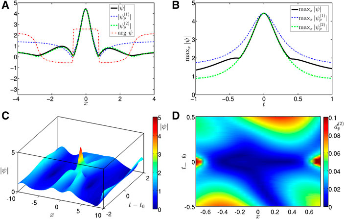
FIGURE 1. (Color on-line) One of the 10 largest RWs (the coordinate of maximum amplitude is shifted to zero for better visualization) for the soliton gas case with time of occurrence $t_0\approx 39.2$, maximum amplitude $A\approx 4.4$ and deviation Eq. 7 from the RBS2 ${\mathcal{D}}_p^{\left(2\right)}\approx 0.02$: (A) space profile of the RW $\left|\psi \left(x,t_0\right)\right|$ at the time $t_0$ of its maximum elevation, (B) time dependency of the maximum amplitude ${\max }_x\left|\psi \right|$, (C) space-time representation of the amplitude $\left|\psi \left(x,t\right)\right|$ near the RW event, and (D) relative deviation Eq. 6 between the wavefield and the fit with the RBS2 in the $\left(x,t\right)$-plane. In the panel (A), the thick black and the thin dash-dot red lines indicate the space profile $\left|\psi \left(x,t_0\right)\right|$ and the phase $\arg \psi \left(x,t_0\right)$. In the panels (A,B), the dashed blue and green lines show the fits with the RBS1 and the RBS2, respectively. In the panel (D), the deviations $d_p^{\left(2\right)}\ge 0.1$ are demonstrated with constant deep red color.

The deviation between a RW and its approximation with a RBS can be measured locally as

$d_p^{\left(\mathrm{1,2}\right)}\left(x,t\right)=\frac{\left|\psi -{\psi }_p^{\left(\mathrm{1,2}\right)}\right|}{\left|\psi \right|}(6)$

Figure 1D shows this deviation $d_p^{\left(2\right)}$ for the RBS2 in the $\left(x,t\right)$-plane: in space–between the two local minimums closest to the maximum amplitude $x\in \Omega$, and in time–in the interval $t-t_0\in \left[-0.5,0.5\right]$, since outside of it the maximum amplitude noticeably deviates from the fit with the RBS2 in Figure 1C. The deviation $d_p^{\left(2\right)}$ remains well within 5% for most of the area demonstrated in the figure, so that the RBS2 turns out to be a very good approximation for the presented RW–simultaneously in space and in time.

As an integral measure reflecting the deviation between a RW and a RBS, one can consider a quantity

${\mathcal{D}}_p^{\left(\mathrm{1,2}\right)}={\left[\frac{{\displaystyle {\int }_{x\in \Omega }{\displaystyle {\int }_{t_0-\Delta T}^{t_0+\Delta T}{\left|\psi -{\psi }_p^{\left(\mathrm{1,2}\right)}\right|}^{2}dxdt}}}{{\displaystyle {\int }_{x\in \Omega }{\displaystyle {\int }_{t_0-\Delta T}^{t_0+\Delta T}{\left|\psi \right|}^{2}dxdt}}}\right]}^{1/2}(7)$

Here we choose the region of integration over time $t\in \left[t_0-\Delta T,t_0+\Delta T\right]$ from the condition that at $t_0\pm \Delta T$ the RBS2 fit halves its maximum amplitude. Indeed, as demonstrated below, the collected RWs have maximum amplitudes roughly between 3.3 and 5, and their halving translates the waves below the RW threshold $\left|\psi \right|>2.8$, see e.g., [19]; also, for most of the RWs, the best fit is the RBS2. For the RW presented in Figure 1, the interval of integration in time is $\left|t-t_0\right|\le 0.31$ and the deviations are ${\mathcal{D}}_p^{\left(1\right)}\approx 0.2$ for the RBS1 and ${\mathcal{D}}_p^{\left(2\right)}\approx 0.02$ for the RBS2.

The quantity Eq. 7 can be used to assess how well a RW can be approximated by a RBS. Figure 2A shows the minimum deviation ${\mathcal{D}}_p=\min \left\{{\mathcal{D}}_p^{\left(1\right)},{\mathcal{D}}_p^{\left(2\right)}\right\}$ vs. the maximum amplitude of the RW $A=\max \left|\psi \right|$ for all 1,000 RWs collected for the soliton gas case; the RWs better approximated with the RBS1 are indicated with the blue squares and those with the RBS2—with the green circles. For 57 RWs the best fit turns out to be the RBS1—the Peregrine breather, while the other 943 RWs are better approximated by the RBS2. According to our observations, the value of the deviation Eq. 7 below 0.05 typically means that such a RW is very well approximated with the corresponding RBS; for $0.05\mathrm{\lesssim }{\mathcal{D}}_p^{\left(\mathrm{1,2}\right)}\mathrm{\lesssim }0.1$ the approximation is satisfactory, and for ${\mathcal{D}}_p^{\left(\mathrm{1,2}\right)}\mathrm{\gtrsim }0.1$—poor. Of 57 RWs better approximated with the RBS1, only four have deviations below 0.1 and none–below 0.05; hence, approximation with the RBS1 turns out to be satisfactory at best. For the RBS2 we have completely different picture: 768 RWs show deviations from the RBS2 below 0.1 and 220—below 0.05. As demonstrated in Figure 2A, larger RWs are typically better approximated with the RBS2. In particular, of 143 RWs having maximum amplitude above 4, 68 have deviation from the RBS2 below 0.05, and the mean deviation for the entire group of 143 RWs is $\langle {\mathcal{D}}_p^{\left(2\right)}\rangle \approx 0.055$. Hence, we can conclude that the largest RWs are typically very well approximated by the RBS2.

FIGURE 2

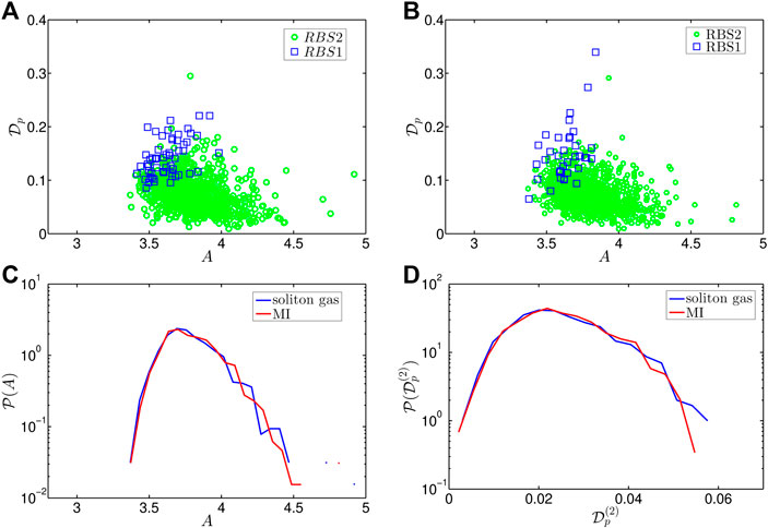
FIGURE 2. (Color on-line) (A,B) Deviation ${\mathcal{D}}_p=\min \left\{{\mathcal{D}}_p^{\left(1\right)},{\mathcal{D}}_p^{\left(2\right)}\right\}$ between RWs and their best fits with either the RBS1 or the RBS2 vs. the maximum amplitude A of the RW: (A) for the soliton gas and (B) for the MI of the condensate close to its statistically stationary state. The blue squares indicate that the best fit is achieved with the RBS1 and the green circles–with the RBS2. (C,D) The PDFs of (C) the maximum amplitude A for all the RWs and (D) the deviation ${\mathcal{D}}_p^{\left(2\right)}$ for the RWs better approximated with the RBS2, for the soliton gas (blue) and the MI of the condensate close to its statistically stationary state (red).

RWs collected close to the statistically stationary state of the noise-induced MI show the same general properties as those for the soliton gas case. Figure 2B demonstrates very similar “clouds” of RWs approximated with either the RBS1, or the RBS2 on the diagram representing the minimum deviation ${\mathcal{D}}_p$ vs. the maximum amplitude A. Of 1,000 RWs in total, 36 are better approximated with the RBS1 and 964—with the RBS2. Of those better approximated with the RBS1, only three have deviations below 0.1 and none–below 0.05. Of 964 RWs better approximated with the RBS2, 792 have deviations below 0.1 and 215—below 0.05. In total, 150 RWs have amplitudes above four; out of them, 64 have deviation from the RBS2 below 0.05, and the mean deviation among the group of 150 RWs equals to $\langle {\mathcal{D}}_p^{\left(2\right)}\rangle \approx 0.059$.

The RWs for the two types of initial conditions turn out to be practically identically distributed by their maximum amplitude, as demonstrated in Figure 2C with the corresponding probability density functions (PDFs). The PDFs of the deviation ${\mathcal{D}}_p^{\left(2\right)}$ for the RWs better approximated by the RBS2 (green circles in Figures 2A,B) are also nearly identical, Figure 2D. Hence, we conclude that the largest RWs for the two systems show practically identical dynamical (resemblance with the RBS2) and statistical properties. Note that we have repeated simulations for the MI case with smaller and larger 1) computational boxes and 2) time windows for collecting the RWs. As a result, we have obtained the PDF of the maximum amplitude shifted to smaller or larger amplitudes, respectively. The nearly perfect correspondence of the two PDFs in Figure 2C additionally justifies the usage of the simulation parameters discussed in the previous Section.

4 Discussion and Future Directions

As we have mentioned in [21]; some two- and three-soliton collisions at the time of their maximum elevation have space profiles remarkably similar to those of the RBS1 and the RBS2. Moreover, we have presented an example of a phase-synchronized three-soliton collision, for which both the space profile and the temporal evolution of the maximum amplitude are very well approximated by the RBS2. The solitons in [21] had nonzero velocities; here we modify the two- and three-soliton examples for the case of zero velocities and also examine the local deviations $d_p^{\left(\mathrm{1,2}\right)}\left(x,t\right)$Eq. 6 together with the integral deviations ${\mathcal{D}}_p^{\left(\mathrm{1,2}\right)}$Eq. 7.

Figure 3 shows an example of three-soliton interaction with solitons having amplitudes $a_1=1$, $a_2=1.5$ and $a_3=2$, zero velocities $v_j=0$, zero space position parameters $x_{0j}=0$ and, at the initial time $t=0$, zero phases ${\Theta }_j=0$. The space profile $\left|\psi \left(x,t_0\right)\right|$ at the time of the maximum elevation $t_0=0$ is remarkably similar to that of the RBS2, and the local deviation $d_p^{\left(2\right)}\left(x,t\right)$ remains well within $5\%$ for most of the area presented in the figure as well. The integral deviation Eq. 7 equals to ${\mathcal{D}}_p^{\left(2\right)}\approx 0.016$, that is even smaller than for the RW presented in Figure 1.

FIGURE 3

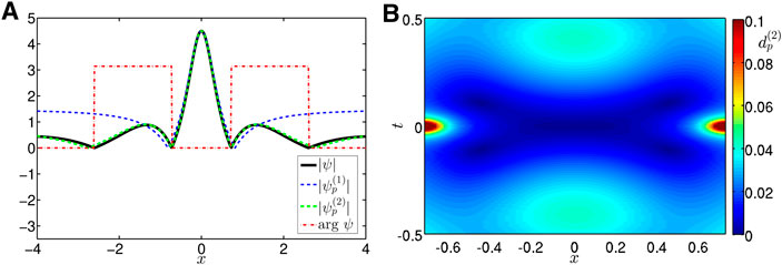
FIGURE 3. (Color on-line) Synchronized three-soliton interaction of solitons having amplitudes $a_1=1$, $a_2=1.5$ and $a_3=2$, zero velocities $v_j=0$, zero space positions parameters $x_{0j}=0$ and, at the initial time $t=0$, zero phases ${\Theta }_j=0$: (A) space profile $\left|\psi \left(x,t_0\right)\right|$ and phase $\arg \psi \left(x,t_0\right)$ at the time of the maximum elevation $t_0=0$, and (B) relative deviation Eq. 6 between the wavefield and the fit with the RBS2 in the $\left(x,t\right)$-plane. All notations are the same as in Figures 1A,D. The deviation Eq. 7 from the RBS2 fit equals to ${\mathcal{D}}_p^{\left(2\right)}\approx 0.016$.

To analyze how often phase-synchronized interactions of two and three solitons of various amplitudes may lead to such quasi-rational profiles, we have created 20 two-soliton and 20 three-soliton interactions with solitons of random amplitudes, zero velocities $v_j=0$, zero space positions parameters $x_{0j}=0$ and phases ${\Theta }_j=0$. For the two-soliton interactions, the minimum deviations from the RBS1 and the RBS2 turned out to be ${\mathcal{D}}_p^{\left(1\right)}\approx 0.077$ and ${\mathcal{D}}_p^{\left(2\right)}\approx 0.061$, and the average ones—$\langle {\mathcal{D}}_p^{\left(1\right)}\rangle \approx 0.14$ and $\langle {\mathcal{D}}_p^{\left(2\right)}\rangle \approx 0.075$, respectively. For the three-soliton case, the minimum deviations were ${\mathcal{D}}_p^{\left(1\right)}\approx 0.18$ and ${\mathcal{D}}_p^{\left(2\right)}\approx 0.003$, and the average ones—$\langle {\mathcal{D}}_p^{\left(1\right)}\rangle \approx 0.23$ and $\langle {\mathcal{D}}_p^{\left(2\right)}\rangle \approx 0.022$; the maximum deviation from the RBS2 equaled to ${\mathcal{D}}_p^{\left(2\right)}\approx 0.03$, that is still very good for comparison with the RBS2. Hence, we conclude that quasi-rational profiles very similar to that of the RBS2 appear already for three-soliton interactions, provided that the solitons are properly synchronized (that is, have coinciding positions and phases).

We think that the presented elementary three-soliton model might provide an explanation of RW formation inside multi-soliton solutions. The most direct way for future studies might be a demonstration of a RW for synchronized many-soliton solution. Here, however, we face a new question, that is, whether formation of a RW is a collective phenomenon that requires synchronization of all the solitons, or a “local” event that can be achieved by synchronizing of a few with arbitrary parameters of the others. Note that even the latter case represents a challenging problem. Indeed, the few solitons that generate a RW acquire space and phase shifts due to the presence of the remaining solitons, that should influence their optimal synchronization condition. For remote solitons, the shifts can be computed analytically using the well-known asymptotic formulas, see e.g., [14]; which however do not work for our case of a dense soliton gas where all solitons effectively interact with each other. This leaves us two options: 1) a local numerical synchronization of a small group with “trial and error” method and 2) calculation of generalized space-phase shifts for closely located solitons. Both ways seem challenging at the moment.

Also note that our study is limited with respect to statistical analysis of RWs, as we have focused on the largest RWs, while the “common” RWs may have different dynamical and statistical properties. Nevertheless, we believe that, since the largest RWs for the two systems show identical properties, the “common” RWs have identical properties too. Identification of all the RWs according to the standard criterion $A\ge 2.8$ is a nontrivial problem by itself, and we plan to return to it in the near future.

5 Conclusion

In this brief report we have presented our observations of RWs within the 1D-NLSE model for 1) the modulationally unstable plane wave at its long-time statistically stationary state and 2) the bound-state multi-soliton solutions representing the solitonic model of this state. Focusing our analysis on the largest RWs, we have found their practically identical dynamical and statistical properties for both systems. In particular, most of the RWs turn out to be very well approximated–simultaneously in space and in time–by the amplitude-scaled rational breather solution of the second order (RBS2), see Figures 1, 2 and the two sets of the collected RWs are identically distributed by their maximum amplitude and deviation from the RBS2, see Figures 2C,D. Additionally, we have demonstrated the appearance of quasi-rational profiles very similar to that of the RBS2 already for synchronized three-soliton interactions, see e.g., Figure 3.

The main messages of the present paper can be summarized as follows. First, a quasi-rational profile very similar to a RBS does not necessarily mean emergence of the corresponding rational breather, as it can be a manifestation of a multi-soliton interaction. Second, the identical dynamical and statistical properties of RWs collected for the two examined systems strongly suggest that the main mechanism of RW formation should be the same, i.e., that RWs emerging in the asymptotic stationary state of the MI (and, possibly, in other strongly nonlinear wavefields) are formed as interaction of solitons. However, more study is necessary to clarify exactly how interaction of solitons within a large wavefield may lead to formation of a RW, and we plan to continue this research in the future.

As future directions of our studies, we consider two problems. The first is about examination of whether formation of a RW in a soliton gas is a collective phenomenon that requires synchronization of all the solitons, or a “local” event that can be achieved by synchronizing of a few. The second problem relates to statistical analysis of all the RWs according to the standard criterion $A>2.8$, in contrast to the largest RWs analyzed in this paper.

Data Availability Statement

The raw data supporting the conclusions of this article will be made available by the authors, without undue reservation.

Author Contributions

All authors contributed significantly to this work.

Funding

The work of DA on simulations and data analysis was supported by the state assignment of IO RAS, Grant No. 0128-2021-0003. The work of AG on generation of multi-soliton solutions and two- and three-soliton models was supported by RFBR Grant No. 19-31-60028.

Conflict of Interest

The authors declare that the research was conducted in the absence of any commercial or financial relationships that could be construed as a potential conflict of interest.

Acknowledgments

Simulations were performed at the Novosibirsk Supercomputer Center (NSU).

References

1. Kharif C, Pelinovsky E. Physical mechanisms of the rogue wave phenomenon. Eur J Mech—B/Fluids (2003) 22:603–34. doi:10.1016/j.euromechflu.2003.09.002

CrossRef Full Text | Google Scholar

2. Dysthe K, Krogstad HE, Müller P. Oceanic rogue waves. Annu Rev Fluid Mech (2008) 40:287–310. doi:10.1146/annurev.fluid.40.111406.102203

CrossRef Full Text | Google Scholar

3. Onorato M, Residori S, Bortolozzo U, Montina A, Arecchi FT. Rogue waves and their generating mechanisms in different physical contexts. Phys Rep (2013) 528:47–89. doi:10.1016/j.physrep.2013.03.001

CrossRef Full Text | Google Scholar

4. Dysthe KB, Trulsen K. Note on breather type solutions of the NLS as models for freak-waves. Physica Scripta, T82 (1999) 48. doi:10.1238/physica.topical.082a00048

CrossRef Full Text | Google Scholar

5. Osborne A. Nonlinear ocean waves and the inverse scattering transform. Cambridge, MA: Academic Press (2010).

6. Shrira VI, Geogjaev VV. What makes the peregrine soliton so special as a prototype of freak waves?. J Eng Math (2010) 67:11–22. doi:10.1007/s10665-009-9347-2

CrossRef Full Text | Google Scholar

7. Peregrine DH. Water waves, nonlinear Schrödinger equations and their solutions. J Aust Math Soc Ser B, Appl. Math (1983) 25:16–43. doi:10.1017/s0334270000003891

CrossRef Full Text | Google Scholar

8. Akhmediev N, Ankiewicz A, Soto-Crespo JM. Rogue waves and rational solutions of the nonlinear Schrödinger equation. Phys Rev E (2009) 80:026601. doi:10.1103/physreve.80.026601

CrossRef Full Text | Google Scholar

9. Kibler B, Fatome J, Finot C, Millot G, Dias F, Genty G, et al. The Peregrine soliton in nonlinear fibre optics. Nat Phys (2010) 6:790. doi:10.1038/nphys1740

CrossRef Full Text | Google Scholar

10. Chabchoub A, Hoffmann NP, Akhmediev N. Rogue wave observation in a water wave tank. Phys Rev Lett (2011) 106:204502. doi:10.1103/physrevlett.106.204502

PubMed Abstract | CrossRef Full Text | Google Scholar

11. Bailung H, Sharma SK, Nakamura Y. Observation of Peregrine solitons in a multicomponent plasma with negative ions. Phys Rev Lett (2011) 107:255005. doi:10.1103/physrevlett.107.255005

PubMed Abstract | CrossRef Full Text | Google Scholar

12. Chabchoub A, Hoffmann N, Onorato M, Akhmediev N. Super rogue waves: observation of a higher-order breather in water waves. Phys Rev X (2012) 2:011015. doi:10.1103/physrevx.2.011015

CrossRef Full Text | Google Scholar

13. Chabchoub A, Hoffmann N, Onorato M, Slunyaev A, Sergeeva A, Pelinovsky E, et al. Observation of a hierarchy of up to fifth-order rogue waves in a water tank. Phys Rev E (2012) 86:056601. doi:10.1103/physreve.86.056601

CrossRef Full Text | Google Scholar

14. Novikov S, Manakov SV, Pitaevskii LP, Zakharov VE. Theory of solitons: the inverse scattering method. Berlin, Germany: Springer Science and Business Media (1984).

15. Gelash A, Agafontsev D, Zakharov V, El G, Randoux S, Suret P. Bound state soliton gas dynamics underlying the noise-induced modulational instability. Phys Rev Lett (2019) 123:234102. doi:10.1103/physrevlett.123.234102

PubMed Abstract | CrossRef Full Text | Google Scholar

16. Belokolos ED, Bobenko AI, Enol’skii VZ, Its AR, Matveev VB. Algebro-geometric approach to nonlinear integrable equations. Berlin, Germany: Springer-Verlag (1994).

17. Bobenko AI, Klein C. Computational approach to Riemann surfaces. Berlin, Germany: Springer Science and Business Media (2011).

18. El GA, Krylov AL, Molchanov SA, Venakides S. Soliton turbulence as a thermodynamic limit of stochastic soliton lattices. Physica D: Nonlinear Phenomena (2001) 152-153:653–64. doi:10.1016/s0167-2789(01)00198-1

CrossRef Full Text | Google Scholar

19. Agafontsev DS, Zakharov VE. Integrable turbulence and formation of rogue waves. Nonlinearity (2015) 28:2791. doi:10.1088/0951-7715/28/8/2791

CrossRef Full Text | Google Scholar

20. Zakharov VE, Mikhailov AV. Relativistically invariant two-dimensional models of field theory which are integrable by means of the inverse scattering problem method. Soviet Phys JETP (1978) 47:1017–1027.

Google Scholar

21. Gelash AA, Agafontsev DS. Strongly interacting soliton gas and formation of rogue waves. Phys Rev E (2018) 98:042210. doi:10.1103/physreve.98.042210

CrossRef Full Text | Google Scholar

22. Zakharov VE, Shabat AB. Exact theory of two-dimensional self-focusing and one-dimensional self-modulation of waves in nonlinear media. Soviet Phys JETP (1972) 34:62.

Google Scholar

23. Lewis ZV. Semiclassical solutions of the Zaharov-Shabat scattering problem for phase modulated potentials. Phys Lett A (1985) 112:99–103. doi:10.1016/0375-9601(85)90665-6

CrossRef Full Text | Google Scholar

24. Kedziora DJ, Ankiewicz A, Akhmediev N. The phase patterns of higher-order rogue waves. J Opt (2013) 15:064011. doi:10.1088/2040-8978/15/6/064011

CrossRef Full Text | Google Scholar

25. Xu G, Hammani K, Chabchoub A, Dudley JM, Kibler B, Finot C. Phase evolution of Peregrine-like breathers in optics and hydrodynamics. Phys Rev E (2019) 99:012207. doi:10.1103/physreve.99.012207

PubMed Abstract | CrossRef Full Text | Google Scholar