Using Topological Data Analysis (TDA) and Persistent Homology to Analyze the Stock Markets in Singapore and Taiwan

In recent years, persistent homology (PH) and topological data analysis (TDA) have gained increasing attention in the fields of shape recognition, image analysis, data analysis, machine learning, computer vision, computational biology, brain functional networks, financial networks, haze detection, etc. In this article, we will focus on stock markets and demonstrate how TDA can be useful in this regard. We first explain signatures that can be detected using TDA, for three toy models of topological changes. We then showed how to go beyond network concepts like nodes (0-simplex) and links (1-simplex), and the standard minimal spanning tree or planar maximally filtered graph picture of the cross correlations in stock markets, to work with faces (2-simplex) or any k-dim simplex in TDA. By scanning through a full range of correlation thresholds in a procedure called filtration, we were able to examine robust topological features (i.e. less susceptible to random noise) in higher dimensions. To demonstrate the advantages of TDA, we collected time-series data from the Straits Times Index and Taiwan Capitalization Weighted Stock Index (TAIEX), and then computed barcodes, persistence diagrams, persistent entropy, the bottleneck distance, Betti numbers, and Euler characteristic. We found that during the periods of market crashes, the homology groups become less persistent as we vary the characteristic correlation. For both markets, we found consistent signatures associated with market crashes in the Betti numbers, Euler characteristics, and persistent entropy, in agreement with our theoretical expectations.

Introduction

The earliest success of econophysics is the application of random matrix theory (RMT, which is a theory combining nuclear physics and statistical mechanics) to the stock market [1–4]. In RMT, one treats noise as a kind of symmetry, and thus information represents some form of symmetry breaking. RMT thus allows physicists to discriminate between noise and signal. The next significant milestone in econophysics is the realization that stock returns follow heavy-tailed Levy distributions [5] instead of a normal distribution. Also, their dynamical properties can be described in terms of fractals (in terms for example, of the Hurst exponent) and multifractals [6, 7] instead of the random walk proposed by Bachelier to model price movements in the stock market. Physicists also love to strip problems down to their simplest essence, using information filtering approaches such as the minimal spanning tree (MST) [8], planar maximally filtered graph (PMFG) [9], triangular maximally filtered graph (TMFG) [10], etc. These represent some of the methodological contributions by econophysicists.

In the PMFG method, important correlations are projected onto a sphere, which has genus g = 0. This is a good starting point for understanding the correlated price movements between different stocks. However, it is possible that the pattern of dynamic correlations may be explainable more naturally in terms of some nontrivial geometrical structure with g > 0. Therefore, the determination of the optimum genus represents a gap in our understanding of correlations in the stock market. This best genus can change with time for the same window length. It can change with window length over the same period, and it can also depend on which market we are looking at. There is also a second gap in our understanding of these dynamic correlations, and that is the problem of overlapping communities. Information filtering methods like the MST and PMFG are not clustering algorithms, but there are clustering algorithms based off them. There are also standard clustering algorithms like k-means and hierarchical clustering that can be used to study the correlation structure in a market. However, all clustering algorithms assume that a stock can be a member-only of one cluster. Ultimately, classifying stocks into clusters help us better imagine the geometry of the correlations, but we do not claim that clusters are independent of each other. We know that within clusters, the interactions are stronger, and between clusters, the interactions are weaker. Recently, researchers started to realize that in many cases, nodes can belong to more than one cluster, giving rise to the problem of overlapping clusters. Currently, the identification of the correct overlapping structures without sacrificing accuracy and speed remains a daunting challenge. These hinder a deeper understanding of co-authorship networks, protein-protein yeast networks, and word association networks. Topological data analysis (TDA) is a method that will kill both birds with one stone. It is ideally suited to 1) identify geometrical structures that are like clusters, and 2) elucidate the weak connections between them.

So how do TDA concepts like simplicial complexes and persistent homology help in filling these gaps? First, once the size of the sliding window is decided, TDA can be quite robust in deciding which topological space or genus to use for projecting the correlation matrices. Indeed, TDA lets the data speak for itself on choosing the optimal topological space and the value of the genus. Second, by appealing to persistency, we do not presuppose which correlation threshold value to use. Instead, we scan through a full range of correlation threshold values, to determine which range the topological structure is most persistent. Third, TDA homologies are very robust to random noises, and as a result, we can avoid technical nuisances such as ‘accumulation of noises’ or ‘overfitting the data’ when clustering data in higher dimensions. Lastly, persistent homology can be presented in the form of persistence barcodes, persistence diagrams, persistence landscapes.

In this paper, our research problem is to use TDA to understand topological changes accompanying crashes in the Singapore and Taiwan stock markets in terms of simplicial complexes, persistent homology, and other metrics. Our hypothesis is that in different market states, different topological features emerge, and TDA can be effective in elucidating these changes. This paper is organized as follows: In Data Section, we briefly introduce how to collect data on the daily returns of the Straits Times Index (STI), the Taiwan Capitalization Weighted Stock Index (TAIEX), and how to preprocess them. In Topology, and Persistent Homology Section we introduce the mathematical background of simplicial complexes, persistent homology, and filtration. In TDA Toolkits Section, we introduce TDA toolkits like barcodes, persistent diagrams, Betti numbers, and Euler characteristics. In TDA of Toy Models and Hypothesis on Real Markets Section, we introduce toy models of TDA and the hypothesis on real markets. In Results and Discussion Section, we show our numerical results computed by TDA and discuss how they confirm our hypothesis. Finally, in Conclusion Section, we give concluding remarks and perspectives.

Materials and Methods

Data

Data Collection

First, we show how to collect price data from stocks in the Singapore Exchange (SGX) [Taiwan Stock Exchange (TWSE)] using Python pandas, and its function web. DataReader, and use the Yahoo Finance API option. Second, to use this option, we need to prepare all the tickers symbols in SGX (TWSE). The procedure is as follows: 1) we go to the ‘My Screeners’ tab in https://sg.finance.yahoo.com/, and choose ‘Singapore’ in the ‘Saved Screeners/Region’ tab, before choosing ‘Find Stocks’ to see a list of ticker symbols. For SGX, there are 672 ticker symbols; 2) copy and save all of them into a file, and 3) using this file of ticker symbols and pandas. web.DataReader’s Yahoo API to fetch historical data between January 1, 2017 and April 30, 2019 from the Yahoo Finance database and save as a CSV file. The Python code to do so is shown in Code 1, and this code can be modified to the TWSE (January 1, 2017 to March 31, 2020) or other markets.

CODE 1.

CODE 1.. A Python code that implements the data collection procedure.

Data Cleaning and Preprocessing

After we collected the raw data, the data needed to be cleaned. First, some ticker symbols are duplicated, so we keep only one copy. Second, for some ticker symbols, the Yahoo Finance API gave an error and caused the program to halt, so we needed to identify these and removed them from the ticker symbol list. Finally, some of the data may include ‘NaN’s and we needed to replace them with ‘0’s. However, if the time series contains more than 50% ‘0’s, we also remove this ticker symbol from the list. After cleaning, we ended up with the times series data for 560 distinct stocks.

Before we computed the cross correlations between stocks from the time-series data to obtain the correlation matrices, three procedures are necessary. First, we standardized the daily prices, which is $\delta x_i=\frac{x_{i-}\overline{x_i}}{\sqrt{{{\displaystyle \sum }}^{\text{}}{\left(x_i-\overline{x_i}\right)}^2/(t-1)}}$, where $x_i$ is the raw stock price for the ith stock, $\overline{x_l}$ is the average stock price for the ith stock, t = 120 is the number of trading days over a six-month period. Second, we smoothed the time series by averaging over a sliding time window of 15 days (for a detailed explanation on why we choose a 15-days window, please see Supplementary Figure S1). Lastly, we converted the daily stock prices to their derivatives, i.e. $\Delta x_i\left(t\right)=\delta x_i\left(t\right)-\delta x_i(t-1)$. In Figure 1A we show the stock price derivatives within a 6-month period after pre-processing, and in Figure 1B, we show the correlation matrix generated from the derivative data. We converted the correlation matrix to a distance matrix using the formula $d_{ij}=\sqrt{2(1-{\rho }_{ij})}$. Finally, we generated distance matrices for successive 6-month periods that are one month apart, to use as input data for subsequent TDA calculations. Other data formats acceptable for TDA include point clouds, networks, or digital images. To be more clear, the procedures are shown in a flowchart (Figure 2).

FIGURE 1

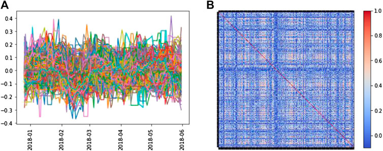
FIGURE 1. (A) The derivative data of a 6-month period collected from STI. (B) The cross correlation matrix is generated from the derivative data in (A). For the time series and correlation matrices in this work, we will not show error bars to not distract the readers from the overall features.

FIGURE 2

FIGURE 2. Flowchart of the procedure implemented. There are two parts; the first part involves data collection and pre-processing. The second part regards TDA-related computations.

Topology, and Persistent Homology

TDA is a mathematical apparatus developed by Herbert Edelsbrunner, Afra Zomorodian, Gunnar Carlsson, and his graduate student Gurjeet Singh [11–13]; it was popularized by Carlsson’s paper [14] that later turned TDA into a hot field in applied mathematics, and also found many applications in data analytics. The foundations of TDA had been laid years before by others in the fields of topology [15–19], group theory [20, 21], linear algebra [22, 23], and graph theory [24–26].

To explain the concept of persistent homology, imagine we have collected a bunch of data points that we refer to as a data cloud. Next, imagine that there is a control parameter called the proximity parameter $\mathit{ϵ}$, which defines the radius of an imaginary ball centered at each of these data points. When we gradually increase $\mathit{ϵ}$, the balls will grow outwards and eventually touch other balls. The overlapping of these balls form a unique topological characteristic that is unique to this dataset, and hence we can use this unique topological characteristic to differentiate nuances in the topologies of different point clouds. This filtration process can be demonstrated and visualized in Figure 3.

FIGURE 3

FIGURE 3. A schematic diagram showing a data cloud, and how the filtration process results in outcomes of various overlapping of balls from different proximity parameters $\mathit{ϵ}$ (shown in the upper column). The bottom column is barcodes scanning through a full-range of proximity parameter $\mathit{ϵ}$ values. β₀ and β₁ denote the 0-dim and 1-dim Betti numbers, which can be deduced from the subfigures to be roughly $18\to 11\to 4\to 1$, and $0\to 0\to 1\to 2$, respectively.

Through this encoding process, we can convert a point cloud that is made from brain functional signals, or a correlation matrix from financial time series data, to filtration diagrams. From these filtration diagrams, we can calculate barcodes, persistence diagrams, and other TDA metrics for further applications.

Simplicial Complexes

A simplicial complex is an abstract collection of entities, which consists of nodes $(i, j, k, \dots )$, or sets of nodes $(\left\{i\right\}, \{i, j\}, \{i, j, k\}, \dots )$. These collections of nodes or sets can then be used to construct links, surfaces, and higher-dimensional objects. For example, we can decompose an arbitrary simplicial complex into its 0-simplexes (nodes), 1-simplexes (links), 2-simplexes (faces), 3-simplexes (tetrahedrons) components. In other words, simplexes are generalizations of a triangle in arbitrary dimensions, and a simplicial complex is an outcome of performing triangulation in arbitrary dimensions of the raw data. The simplicial complex is a unique signature that characterizes the topological structure of the data. Some of the common simplicial complexes include Vietoris-Rips (VR) complexes [27], Čech complexes [16, 18], Delaunay complexes [28], Alpha complexes [29], witness complexes [30], as well as others. In this work, we used the VR complex for our TDA calculations. VR is appealing because it approximates the more exact Čech complexes but is more efficient to calculate [31].

Suppose we collected two sets of time-series data of the same duration from a stock market. After we encode them into simplicial complexes, these may be different in terms of their local and global topologies. We then can use TDA metrics such as Betti numbers, Euler characteristics, barcodes, persistence diagrams, persistence landscapes, and Wasserstein distance as topological descriptors to quantify these differences. In the following subsections, we introduce some of these terminologies, their respective definitions, and elaborate on them.

Filtration

Here let us formalize the definition of the filtration procedure, which is commonly done to obtain barcodes. By changing the proximity parameter $\mathit{ϵ}$, we control the size of the balls and thus their overlaps. At a specific $\mathit{ϵ}$ value, some balls overlap while others do not, and therefore we have a collection of 0-simplexes (isolated nodes), 1-simplexes (pairs of linked nodes), 2-simplexes (triangles), 3-simplexes (tetrahedrons), and so on. Such a collection is called a sub-complex. If we increase $\mathit{ϵ}$ further, the sub-complex (and its topological features) may or may not change. This procedure resembles what we see in physics: by changing the external fields, e.g. temperature, or magnetic fields, the system changes from one symmetry group to another. We call this symmetry breaking. A filtration is conceptually similar to varying the external fields, and observe how they result in different symmetry groups. The difference is that in performing filtrations, we look at how the topological features evolve. Mathematically, a filtration can be described as a sequence

$\varnothing ={\Sigma }^0\subseteq {\Sigma }^1\subseteq {\Sigma }^2\cdots \subseteq {\Sigma }^m=\Sigma \text{, }$

where ${\Sigma }^m=\Sigma$ is the simplicial complex, $\varnothing ={\text{Σ}}^0$ is the empty set, and ${\Sigma }^k\subseteq {\Sigma }^{k+1}$ indicates that the kth sub-complex is included in the (k+1)th sub-complex. In performing the filtration, we witness at that at $\mathit{ϵ}={\mathit{ϵ}}_k$, there is a topological transition from ${\text{Σ}}^k$ to ${\text{Σ}}^{k+1}$. By tracking all these ${\mathit{ϵ}}_{kS}$, we know how the simplicial complex’s topology changes. We can then characterize these topological changes in terms of Betti numbers, Euler characteristics, barcodes, persistence diagrams, and persistence landscapes.

TDA Toolkits

Homology Group

In a filtration process, one can imagine that for smaller $\mathit{ϵ}$, the data points will have lesser overlaps; while we increase $\mathrm{ϵ}$ further, balls start to grow in size and eventually touch other balls, resulting in more overlaps; this continues until $\mathit{ϵ}$ become so large that all the balls overlap with each other, leaving no space for holes to persist. Thus, for an intermediate $\mathit{ϵ}$, we expect to see balls making some overlaps but not too much, and the extents of these overlaps constitute different topological characteristics in terms of ‘n-dimensional holes’. Homology is a mathematical theory for studying these n-dimensional holes that exist in simplicial complexes by identifying which entities constitute these n-holes, and how many there are.

As mentioned before, SCs are obtained from performing a triangulation in arbitrary dimensions of the input data, or a way to represent the data in terms of ‘sets’. But looking at sets is sometimes hard to develop an overall, comprehensive picture of the data, and also less convenient for executing mathematical operations on them. For this reason, mathematicians convert SCs, and other topological sets into groups, rings, or fields, so that in these constructs, they not only can discern between different sets, but also can impose structures like associative binary operations, the identity element, and the inverse element on them. See Figure 4 for the procedures of encoding the raw data into sets, TDA metrics, allowing for further applications.

FIGURE 4

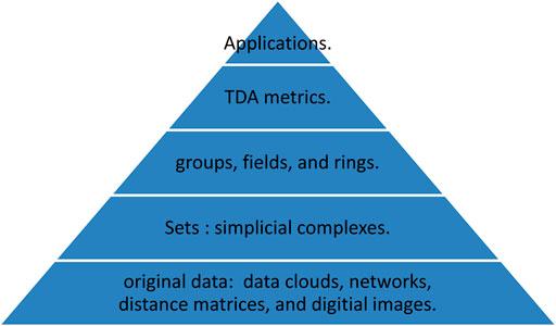
FIGURE 4. A pyramid illustrating sequential procedures of how we make use of the original data and convert them into different forms of sets, i.e. simplicial complexes, and to groups, fields, and rings. At the topmost stage, we can use them for various applications, such as ML, and statistical learning, etc.

Unlike manifolds, which are continuous sets of points, SCs comprise discrete points instead. Although both can describe topological features in the data space, there is one advantage in using SCs, and that is one uses a triangulated (coarse-grained) surface instead of a continuous one. Practically, we are interested only in the n-holes and their numbers, and we only have limited data. In this sense, SCs and their homology are adequate to fulfill these goals.

Betti Numbers and Euler Characteristics

An Euler characteristic is used to classify different polyhedrons, it reads:

$\text{χ}=V-E+F=2\left(1-g\right)\text{,}$

where χ is the Euler characteristic of a polyhedron, V, E, and F are the numbers of nodes, links, and surfaces, respectively. In this formula, g is the genus of the polyhedron. χ can also be calculated as a sum of Betti numbers,

$\chi ={\displaystyle \sum _{\left\{\text{n}\ge 0\right\}}{\left(-1\right)}^n{\beta }_n\left(\Sigma \right)}\text{,}$

where the nth dimensional Betti number β_n is the dimension of the nth homology group $H_n\left(\Sigma \right)$ of the SC $\Sigma$. These are important metrics that characterize the topology of the data.

Barcodes and Persistence Diagrams

Barcodes help us visualize the n-dimensional homology group ${\text{H}}_{\text{n}}\left(\Sigma \right)$ in terms of its generators. We understand that each bar represents a generator of the persistent homology group $H_n^{\left\{p,q\right\}}\left(\Sigma \right)$. This representation tell us that the number of bars that are born at or before the pth filtration stage that are still alive at the qth filtration stage is precisely the rank of $H_n^{\left\{p,q\right\}}\left(\Sigma \right)$, which includes the essential classes that do not die with filtration [32].

The rank of the homology group in nth dimensions equals the nth Betti numbers, which we use to calculate the Euler characteristics $\text{χ}$. For more persistent bars, their topological features are more important, whereas the topological features of those that are less persistent can be treated as noises. Here, we convert the barcodes into persistence diagrams in Figure 5. Persistence diagrams carry similar topological information as barcodes. It is more useful in constructing statistical topological models that can be used to design weighted kernels.

FIGURE 5

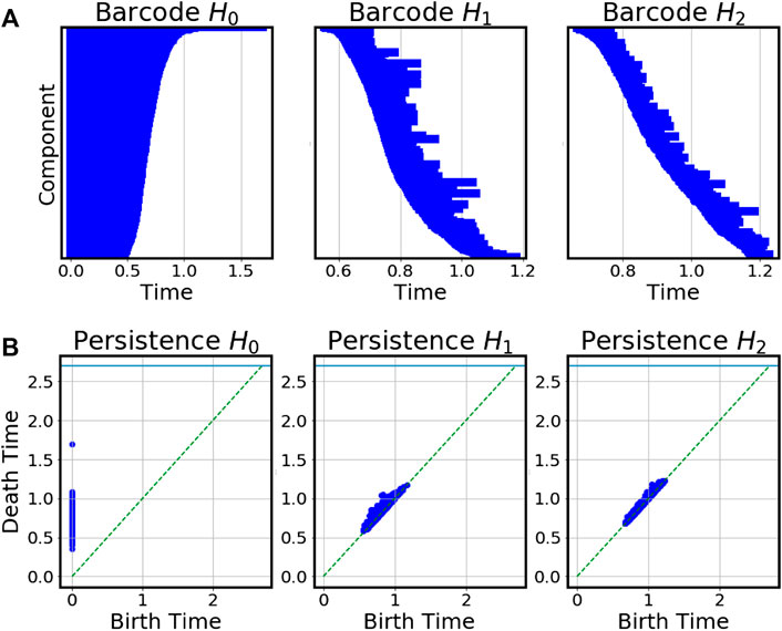
FIGURE 5. (A) Barcodes in 0, 1, and 2 dimensions. Each bar represent a generator of the homology group, i.e. $H_n^{\left\{p,q\right\}}\left(\Sigma \right)$, where {p, q} marks a lifetime, the rank of $H_n^{\left\{p,q\right\}}\left(\Sigma \right)$ equals Betti number of homology groups in the nth dimension, the length of {p, q} signifies the persistence of the nth Betti number. (B) The barcodes can be converted into persistence diagrams, where one of the bars in (A) is equivalent to one point in the persistence diagram. The lifetime of each bar in (A) can be transformed into a perpendicular distance concerning the diagonal lines in (B). If A point that is farther away from the diagonal line implies a more persistent topological feature, whereas a point that is closer to the diagonal line represents a less persistent feature. We found that the barcodes are rather robust and do not show fluctuations once the dataset is fixed, thus we do not include error bars in all barcodes appearing in this paper.

Computational Methods

TDA Toolkits

Numerically, we used two softwares to perform the TDA calculations. The first software is called Ripser [33], which is included inside the Python package TDA [34]. Another is a Java program called Javaplex [35], which we used to calculate Betti numbers and Euler characteristics. Javaplex supports parallel computation in MPI and OpenMP, shortening the computing time for calculating persistent homology in higher dimensions. We installed Javaplex on Nanyang Technological University High-Performance Computing Centre’s NYA2, equipped with Sandy-Bridge Processors-cores (Intel(R) Xeon(R) CPU E5-2680 @ 2.70 GHz), and 64 GB RAM per Node. NYA2 runs Red Hat Enterprise Linux Server release 6.3 (Santiago) and manages job queues using the Load Sharing Facility (LSF).

For some of the time windows, the Javaplex calculations failed with the error message “OutOfMemoryError: Java heap space” and “OutOfMemoryError: GC overhead limit exceeded”. Here we offer two solutions. The first is to utilize more than 100 GB of memory on client computers, which can be switched on by adding a line “#BSUB -q MEM128G-S” in the LSF script. This option allows the submitted jobs to access up to 128 GB of memory. If the first solution fails, a second solution is to reduce the upper limit of the filtration value, say a value near 1.0. These two options can in general solve the problem of the memory shortage issue. On average, a job submitted to NYA2 accessing 16 CPU cores requires 1–3 days to finish. For each of the calculations, we saved barcodes figures, n-dimensional Betti numbers, Euler characteristics in separate folders for further analysis.

TDA of Toy Models and Hypothesis on Real Markets

Before we analyze the SGX and TWSE data, and discuss their results, as a proof-of-concept we first digress to demonstrate the main idea behind our work by applying TDA to three toy models with definite topological changes. In these three cases, we randomly sampled data points on the surfaces or in the volumes and then saved these data points in separate files. Then, we use the Javaplex software to read in the files and calculate the persistent homology and respective Betti numbers up to dim 2. Finally, we use $\chi ={\displaystyle \sum }_{\left\{\text{n}\ge 0\right\}}{\left(-1\right)}^n{\beta }_n\left(\Sigma \right)$ to calculate the Euler characteristic. These results are shown in Figure 6.

FIGURE 6

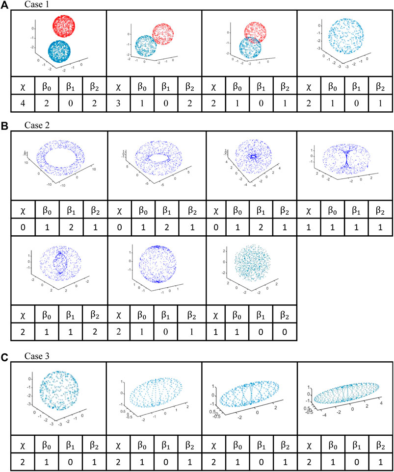
FIGURE 6. The toy models illustrating three different sequences of topological changes. (A) We start with two spherical shells of radius one and move them closer until their surfaces touch, overlap, and finally merged into a larger single spherical shell. (B) We generate a sequence of surfaces of revolution that starts with a torus, then one with a smaller hole, then a horn torus, a spindle torus, and finally a spherical shell. We also show a solid sphere. (C) We start with a spherical shell and then deform it into ellipsoids, whose semi-axis we increase from $5\to 10\to 20$.

In the first case (Figure 6A), we started with two spherical shells of radius one that do not overlap. We then moved the two shells closer until their surfaces touch, before we moved them even closer that they overlap. For this sequence of configurations, we saved the data points and thereafter invoked the Javaplex software. In the third, overlapping configuration, we manually deleted those data points that lie inside the spherical shells. Finally, we compared this sequence of configurations against a larger spherical shell. We found that χ went from $4\to 3\to 2\to 2$, which was consistent with the analytical results. The sequences of Betti numbers provided even more information. As we went through the sequence of configurations, β₀ changed from $2\to 1\to 1\to 1$, which agrees with what we expected, since β₀ tells us how many connected components there are in the configuration. We also found β₁ = 0 throughout the sequence, since it is the number of irreducible closed loops, and in all configurations, we can always shrink a closed loop to a point. Finally, we found β₂ changing from $2\to 2\to 1\to 1$, since it is the number of voids enclosed within the different surfaces, so this becomes 1 after the two spherical shells overlap.

For the second case (Figure 6B), we went through a sequence of surfaces of revolution of two circles at increasing closer distances. When the two generating circles were far apart, we obtained a torus with a big hole, and when the two generating circles were closer but still non-overlapping, we obtained a torus with a small hole. When the two generating circles touched each other, we ended up with a horn torus, which is a critical surface with no holes but is pinched at a point. When the two generating circles overlapped each other, we obtained a spindle torus, which has an inner as well as an outer surface. Finally, when the two generating circles overlapped completely, we obtained a spherical surface. This last configuration is then compared against a solid sphere. For this sequence, we found χ going from $0\to 0\to -4\to -1\to 2\to 1$, which is the result of an interesting interplay between the Betti numbers. Going through the sequence, we found β₀ = 1 throughout, because there is only one connected object. In contrast, β₁ went from $2\to 2\to 5\to 3\to 0\to 0$ and β₂ = 1 for all configurations, except for the spindle torus (β₂ = 2), and the solid sphere (β₂ = 0). Since β₂ is the number of voids enclosed, we understand why β₂ = 1 for the spherical shell configurations, and why β₂ = 2 for the spindle torus. In this sequence, the most interesting change occurred in β₁.

For the final case (Figure 6C), we started with a spherical shell and increased its eccentricity to get longer ellipsoids, with semi-axis a going from $5\to 10\to 20$. For all these different ellipsoids, we found that χ = 2, confirming the fact that deformation alone cannot change the topology or the Euler characteristic. We also found β₀ = 1, β₁ = 0, and β₂ = 1 for all these surfaces, as expected.

For all cases, we also computed the corresponding barcodes and persistent diagrams for better insights into how they evolve with topological deformations. These are shown in Supplementary Figure S2.

Generally speaking, the cross correlations in a stock market will be in the form of a high-dimension topological space, with more complicated features than those shown above. Nevertheless, we believe the insights derived from the toy models can help us grasp the topological changes that occur during a stock market crash (shown schematically in Figure 7). Just before the market crash (Figure 7A), we show the cross correlations of the stock market as a single giant cluster with four holes, which tells us that β₀ = 1 and β₂ = 4, while β₁ will depend on the detail shape of the topological surface. This strongly interconnected situation is typically generated by a bubble in the market and can be viewed as the starting point of a market crash [36, 37]. When the market crash starts (Figure 7B), parts of the surface will break (red circles in Figure 7B) but overall the giant cluster remains. The breaking of these two handles results in β₂ going from 4 to 2, while β₀ remains 1. For every handle broken, β₁ also decreases by 2. As the market crash progresses, the giant cluster starts to crumble, giving rise to additional small clusters like the ones shown in Figure 7C. When the number of connected components increases, β₀ goes from 1 to 5, and β₂ decreases further to 1, because there is only one hole remaining. The small clusters do not contribute to β₂ if they are homomorphic to spheres. Finally, at the end of the market crash, many small clusters are produced by the dissociation of the giant cluster, so β₀ increases dramatically, but β₁ and β₂ become small. Such a cluster fusion-fission scenario has been proposed previously [38, 39], but we suspect TDA will provide additional information regarding subtle topological changes that these models cannot provide.

FIGURE 7

FIGURE 7. A schematic diagram illustrating different states in the stock market across a market crash. (A) All stock components are interconnected and form a single giant cluster with holes. (B) As the market starts to crash, some of the connections are broken, but the single giant cluster remains as in case (A). (C) As the market crash progresses, the giant cluster remains, but part of it has fragmented into four smaller clusters. (D) At the end of the market crash, the stocks are now organized into many small and disjoint clusters.

Armed with these insights, we proceed next to the research question, that is to use TDA to examine the topological changes associated with market crashes in the SGX and TWSE, to see how well our hypothesis holds out.

Results and Discussion

In this work, we examined two stock markets, i.e. the Singapore Stock Market (STI), and the Taiwan Stock Exchange (TAIEX). Both markets consist of roughly 600 stock components, and the economic scales of Taiwan and Singapore are comparable. The time durations that we collect data are from Jan 2017 to Apr 2019 for STI, and from Jan 2017 to March 2020 for TAIEX. For TAIEX, there is a small market crash from Sep 2018 to Jan 2019, and a major crash in Mar 2020 that is caused by the COVID-19 pandemic, whereas no market crash was found for the STI.

Correlation Matrices

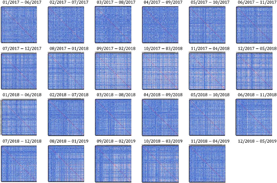
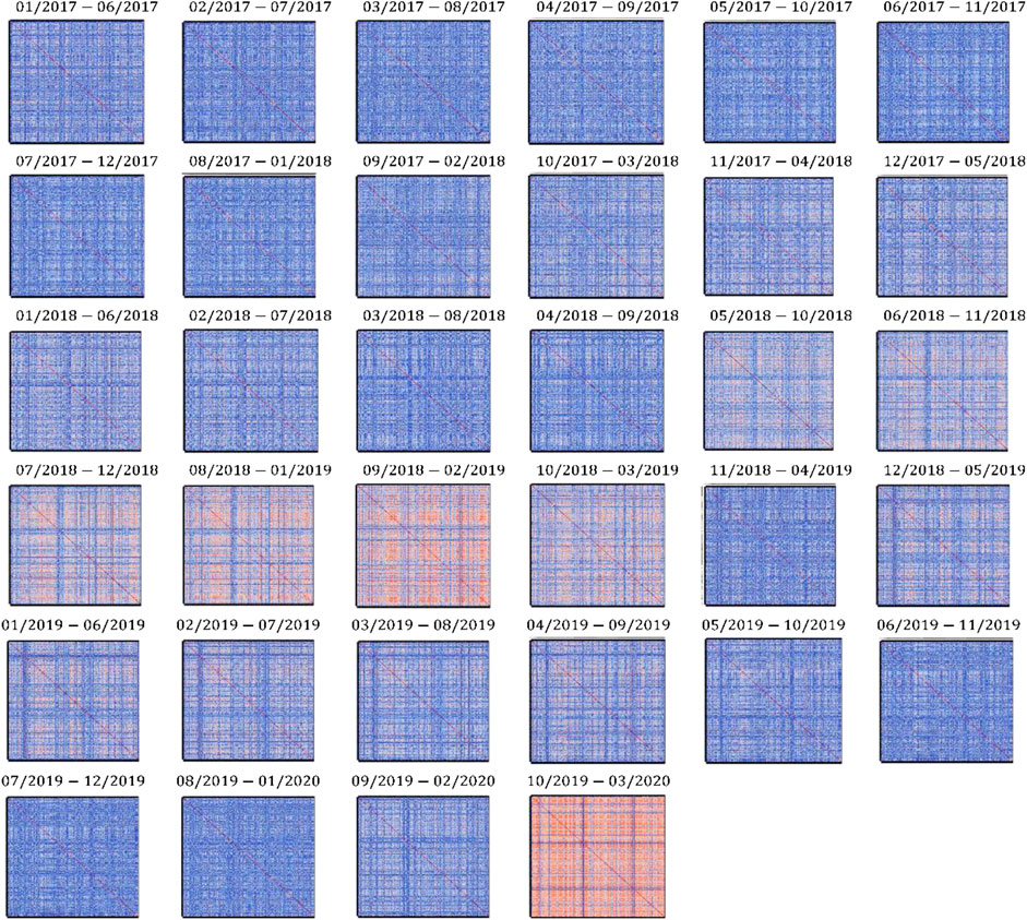
We visualize the complex dynamics in the two stock markets by computing correlation matrices over six-month periods that are one month apart. We used a heat map color scheme, where the highest correlation value of 1 is red, and the most negative correlation of −0.1 is blue. These are shown in Figures 8 and 9 for STI, and TAIEX.

FIGURE 8

FIGURE 8. The correlation matrices of STI from Jan 2017 to Apr 2019.

FIGURE 9

FIGURE 9. The correlation matrices of TAIEX from Jan 2018 to Mar 2020.

In Figure 8 for STI, it is clear that the average correlation is low over most periods. The exceptions are the periods (Sep 2017, Feb 2018), (Oct 2017, Mar 2018), (Nov 2017, Apr 2018), and (Dec 2017, May 2018). In Figure 9 for TAIEX, however, we observe more drastic changes. The correlation matrix first becomes reddish for the (May 2018, Oct 2018) period, and remains reddish until the (Oct 2018, Mar 2019). It then became reddish again in the (Oct 2019, Mar 2020) period because of the COVID-19 pandemic. Particularly, the few correlation matrices preceding the COVID-19 crash were blue, making the reddening very sudden.

In the literature, spectral reddening can be used as early warning signals to inform critical transitions [40–43]. Before market crashes, the co-movement among stocks becomes stronger, variations become increasingly concentrated at low wavenumbers, and result in a reddish color in the spectral density. Although inspecting different properties, both show early warning signals by turning into red colors when approaching these critical transition points.

Barcodes and Persistence Diagrams

The barcodes and their corresponding persistence diagrams for TWSE data between Apr 2019 and Sep 2019 are shown in Figure 10. In Figure 10, the left three figures are the barcodes in 0-dim, 1-dim, and 2-dim, respectively, whereas the right three figures are the corresponding persistence diagrams. In the right three figures, the x-axis refers to the time of birth, while the y-axis refers to the time of death for each homology group, represented by a dot on the figures. We also use red arrows to indicate which bar in the left figures corresponds to which dot in the right ones. When the period is varied, the shape of these figures also changes, revealing the dynamics of the topological structures.

FIGURE 10

FIGURE 10. The barcodes, and corresponding persistence diagrams for data collected from Apr 01, 2019 to Sep 30, 2019 in TAIEX.

For the persistence diagrams, the dots in the 0-dim figure only move vertically in time, whereas for those in 1-dim, and 2-dim, the data points can cluster together forming a small bump, flatten out along the diagonal line, or translate toward or away from the origin along the diagonal line. During market crashes, intriguing dynamical properties can be seen in these figures. To make a clearer comparison, we show in Figure 11 the aggregated STI and TAIEX 5-years historical data and discuss the features seen in Supplementary Appendix Figure A1 and Supplementary Appendix Figure A2, where we show all the barcodes and persistence diagrams for the data collected from SGX and TWSE.

FIGURE 11

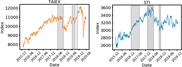
FIGURE 11. The (A) TAIEX and (B) STI index for the past five years, which include the period we collected our data. For TAIEX, the period is from Jan 01, 2017 to Mar 31, 2020. For STI, the period is from Jan 01, 2017 to Apr 30, 2019. In this figure, the gray bands are periods seen from Figure 14 where the Euler characteristic is positive.

In Figure 11A, we find a local market minimum from Sep 2018 to Jan 2019, spanning roughly five months following a small crash in Sep 2018. From the barcodes and persistence diagrams in Supplementary Appendix Figure A1, we discover an interesting feature related to this small crash. When we compare the 1-dim and 2-dim persistence diagrams for the (Mar 2018, Aug 2018) period (not including the crash) against those of the (Apr 2018, Sep 2018) (including the crash) in Supplementary Appendix Figure A1, the data points flatten out along the diagonal line, suggesting that in these two dimensions, the persistence of the homology groups weakens. However, the 0-dim result shows no signs of change when we compare these two subfigures. This episode of a persistence-weakening in 1-dim and 2-dim continued until the (Oct 2018, Mar 2019) period in Supplementary Appendix Figure A1 when the flattening-out phenomenon disappears. Looking at the barcodes in the same period, we witnessed that the 1-dim and 2-dim bars, which are generally wider before the (Mar 2018, Aug 2018) period, becoming visibly shorter in the period (Apr 2018, Sep 2018) to (Oct 2018, Mar 2019). To aid visualization, we used red-shaded windows in Supplementary Appendix Figure A1 to identify those barcodes manifesting persistence weakening. In the Supplementary Figure S4, we also show schematically how bars in the barcodes become dots in the persistent diagram during a normal market phase and a market crash phase.

We observed an even stronger persistence weakening for the (Oct 2019, Mar 2020) period than for the small crash. Going back to the barcodes, we found the widths of the bars becoming smaller as the distribution of data points flatten in the persistence diagram. We also found a large gap of $1.2<\mathit{ϵ}<1.4$ between the death of one bar, and the birth of the next bar in the 2-dim barcode. To unravel how this persistence-weakening phenomenon occurs, we reduced the time windows’ sizes to 2, 3, 4, and 5 months, and show the results in Figure 12.

FIGURE 12

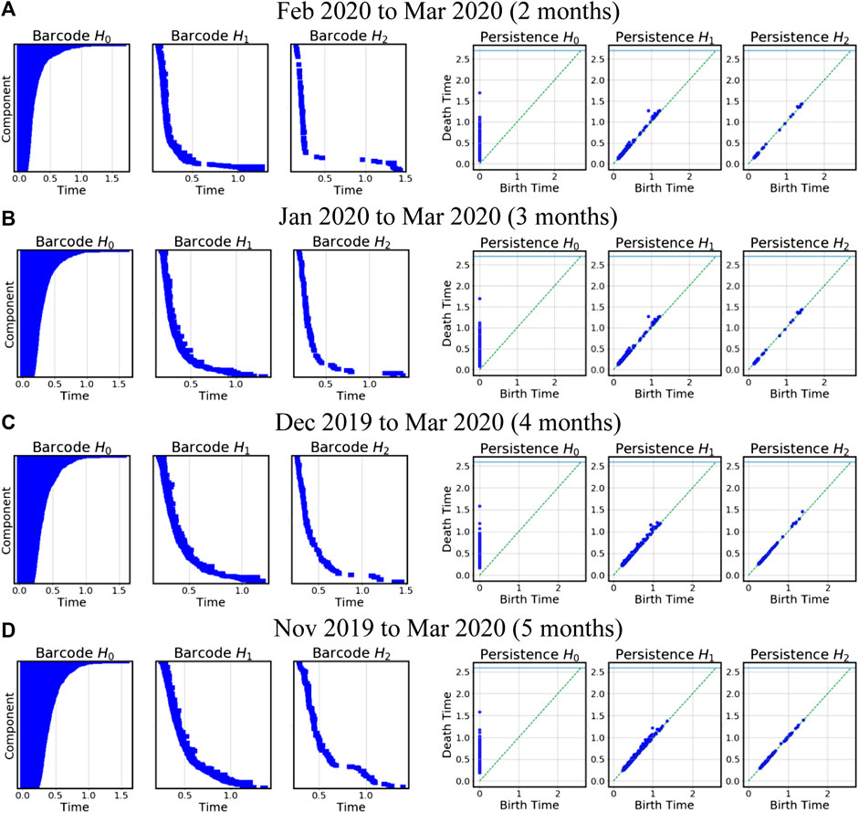
FIGURE 12. The barcodes and persistence diagrams covering the pandemic COVID-19 crash in March 2020. The first column is a two-month window result, and the subsequent columns correspond to 3, 4, 5, and 6-months time windows, respectively.

In Figure 12, we witness some interesting features. First, in the 0-dim persistence diagram, the dots seem to be lower compared to those periods without market crashes. This corresponds to a shorter life expectancy for the homology groups, which can also be observed in the barcodes. In the 1-dim and 2-dim barcodes, we find the barcodes falling off rapidly between $\mathit{ϵ}=0$ and $\mathit{ϵ}=0.2$, and more slowly thereafter. This suggests that $\mathit{ϵ}=0.2(\rho =0.97)$ is a characteristic scale that emerged only during the COVID-19 crash. To quantify the persistence-weakening phenomena in TWSE, we selected three periods and analyzed the H₁ and H₂ persistence diagrams (see Supplementary Figure S3). In the normal market state during the six periods (Jan 2017, Jun 2017) to (Jun 2017 to Nov 2017), the two principal variances were found to be ${\sigma }_1^2=0.361\pm 0.036$, and ${\sigma }_2^2=0.066\pm 0.003$ for H₁. For H₂, we found that ${\sigma }_1^2=0.371\pm 0.07$, and ${\sigma }_2^2=0.036\pm \text{0}\text{.}001$. For the period (Sep 2018, Feb 2019), which covers the mini-crash, we measured ${\sigma }_1^2=0.763$, and ${\sigma }_2^2=0.046$ for H₁; for H₂, we measured ${\sigma }_1^2=0.860$, and ${\sigma }_2^2=0.024$. Finally, for the period (Oct 2019, Mar 2020), we obtained ${\sigma }_1^2=0.770$ and ${\sigma }_2^2=0.041$ in H₁; for H₂, ${\sigma }_1^2$ increased to 0.931, while ${\sigma }_2^2$ become 0.020. To conclude, during the two market crashes in TWSE, the second principal variance was reduced, implying a shortened persistence lifetime, a manifestation of the persistence-weakening phenomena that come along with crashes.

Another way to quantify the persistence weakening is through the persistent entropy, $E\left(F\right)=-{\displaystyle \sum }_{\text{i}=1}^{\text{n}}{p}_i\text{log}\left(p_i\right)$ where F is the distribution of lifetimes $l_i=y_i-x_i$ (x_i, y_i are the birth time and the death time of homology group i in the barcode with n segments), $S_L={\displaystyle \sum }_i^n{l}_i$ is the sum of all lifetimes, and $p_i=l_i/S_L$ can be thought of as the ‘weight’ of homology group i in the barcode [44, 45]. The persistent entropy E(F) is maximum when all homology groups have the same lifetimes, and is minimum when the lifetimes of homology groups are all different. E(F) thus allows us to distinguish between narrow and broad distributions of lifetimes, as well as smoothly varying and multimodal distributions of lifetimes. We chose to compute E(F) for the same three periods used to calculate the covariance matrix and principal variances. For the normal market state during the six periods (Jan 2017, Jun 2017) to (Jun 2017 to Nov 2017), we found that $E\left(F\right)=2.8185\pm 0.004, 2.741\pm 0.028, 2.733\pm 0.072$ in 0–2 dim respectively; for the period (Sep 2018, Feb 2019), E(F) remained roughly the same at 2.80 for 0-dim, but decrease to 2.55 for 1-dim, and more significantly to 2.1 for 2-dim. For the COVID-19 crash, E(F) for 0-dim remained at 2.80, while for the other two dims, they became 2.40 and 1.94. This suggests that E(F) for 2-dim changes most dramatically across market crashes.

For SGX (Supplementary Appendix Figure A2), the persistence-weakening phenomena are less significant, except for (Sep 2017, Feb 2018), (Nov 2017, Apr 2018), and (Dec 2017, May 2018). In these periods, persistence-weakening only occurs in the 2-dim persistence diagrams but not in their 1-dim counterparts. This is rather different from those observed in the two TAIEX crashes. We believe this is because over the period Jan 2017 to Apr 2019, the largest downward movement of the STI is still smaller than the smaller TAIEX crash, as such the persistence weakening is less prominent. Referring to Figure 11B, we believe these downward movements were market corrections in the STI, and the analysis we introduced thus far cannot help to classify them. Consequently, we introduce the Betti numbers and Euler characteristics in the next subsection to resolve this issue.

Other Works Addressing Persistence

In 2015, Teh and Cheong [38] studied dynamics in the SGX during the Global Financial Crisis using a cluster fusion-fission approach. They found that before the crisis, a giant cluster of stocks emerged in the SGX. This later broke up into small clusters after Lehman Brothers went bankrupt. Also, they found that the probability that a pair of stock remain in the same cluster decays exponentially with two time scales i.e. 3 weeks, and 7 weeks. They called these temporal correlations the ‘persistence’ of stocks. In our work, since our sliding window size is one month, we can also measure the persistence in both time scales, in terms of n-holes that emerge in the two-time windows.

We show the mean value of bottleneck distance D (we pick three points in Jan 2017 as origins, and calculated D with subsequent n = 11 months for the origin), and its standard deviation in SGX over the whole of 2017 in Figure 13. We discovered that D increased steadily over the next four windows for H₀, and then saturated around 0.25, whereas for H₁ and H₂, D also increased but less significantly over the n-windows. A larger D implies that the homology groups are less persistent, whereas the converse means the persistence is stronger. As for the case of TWSE, we investigated two periods. The first period is (Jan 2017, Dec 2017), the same as the first period studied for the SGX, and the second is (Sep 2017, Aug 2018), which is in the middle of the mini-crash. For these two periods, we observe dissimilar features for H₀. In the first period, D grew from an initial value of 0.05, and saturated around 0.2, before dropping steeply to 0.07. For the second period, H₀ stayed between 0.13 and 0.15, before jumping to a larger value of roughly 0.22 seven months later. As expected, the bottleneck distance increases and then decreases over the course of a market crash.

FIGURE 13

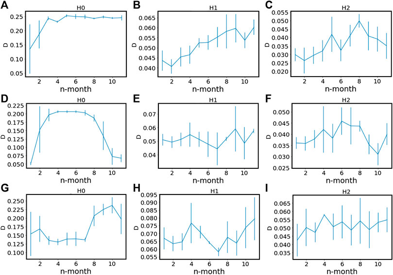
FIGURE 13. Bottleneck distances D calculated for (A)H₀, (B)H₁, and (C)H₂ for the origin month (we pick three points in Jan 2017 as origins, and calculated D with subsequent n = 1 months). The solid lines are the mean values, and the vertical bars are the standard deviation for each data point. (D–F) are the same as (A–C) but for normal market states of TAIEX, and (G–I) we select three points in Sep 2018 as origins, and calculated D with subsequent n = 11 months, covering the mini market crash of TAIEX.

kth Betti Numbers and Euler Characteristics

In the literature, econophysicists use cross correlations to distinguish between different market states, like the bull and bear market states, as well as the market correction state. In a market correction state, the market condition resembles a random walk process, and thus the cross correlations between stocks are random matrix-like, and the distribution of their eigenvalues resembles a Marčenku–Pastur distribution (MPD). Following Reimann et al. and Santos et al. [46, 47], we can also use the kth Betti numbers and Euler characteristics as fingerprints to classify market states in the STI and TAIEX. According to Reimann et al. and Santos et al., different correlation matrices can have higher similar fingerprints and thus represent the same topologies.

In [46, 48], the authors also proposed to use the Euler entropy $S_x=\ln \left(\left|\chi \right|\right)$ as an alternative entropy construct, instead of the conventional Boltzmann entropy. They used the Euler entropy to inform whether there are topological phase transitions at any specific time or correlation values. According to their findings, a negative χ can be geometrically connected to a sheet of hyperboloid with negative curvature, at χ = 0 the hyperboloid become cone-like, on the edge of breaking into two hyperboloids, and finally a positive χ, where the hyperboloid breaks into two hyperboloids. Hence, when χ changes from a positive value to a negative one, we can identify a critical point. At these points, the Euler entropy explodes $\left(\ln \left|0\right|\to -\infty \right)$ and become singular. In statistical mechanics, when the system approaches a critical point, we expect to see the susceptibility function become non-analytic. In view of this, we can also use the Euler entropy to analyze and classify different market states.

Here, we show the kth Betti number and Euler characteristics for different periods in the SGX (TWSE) in Table 1. For TWSE, we chose two periods of time, i.e. (Jun 2017, Dec 2018), and (May 2019, Oct 2019), to calculate χ. These periods correspond to the two TAIEX crashes. Also, we calculated up to 2-dim Betti numbers, because for TWSE, we were not always able to compute the 3-dim Betti numbers. From July 2018 to Nov 2018, we found that χ was positive, and become negative in Dec 2018. From June 2019 to Sep 2019, χ stayed close to zero, and then suddenly jumped to 98 in Oct 2019, whose time window included the COVID-19 crash in Mar 2020. Based on our results, both crashes seem to be associated with large positive χ values instead of negative ones. We can understand a positive χ as the result of many isolated hyperspheres, while a negative χ comes from averaging the curvature over hyperbolic bridges after some hyperspheres merged. This conclusion is also supported by the behavior of β₀, whose average values over the two periods are 31.6 and 98 respectively, suggesting that the stock components are fragmented rather than agglomerated. On the other hand, while χ is 23 and 27 respectively for (June 2018, Nov 2018) and (Jul 2018, Dec 2018), the values for β₀, β₁, and β₂ are different, implying that their topologies are dissimilar. Our findings agree with our hypothesis that during crashes, stock components tend to break up into fragments, even though the overall cross correlations are high.

TABLE 1

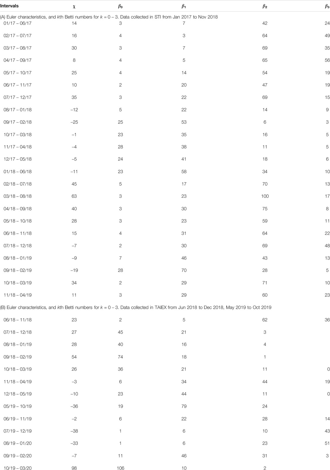
TABLE 1. (A) Euler characteristics, and kth Betti numbers for $k=0-3$. Data collected in STI from Jan 2017 to Nov 2018. (B) Euler characteristics, and kth Betti numbers for $k=0-3$. Data collected in TAIEX from Jun 2018 to Dec 2018, May 2019 to Oct 2019. Two periods cover the two crashes. We have calculated β_k specifically for the period in TAIEX (Jan 2017 to Jun 2017) 10 times to test if β_k fluctuates; our results confirmed that all arrived at the same β_k and χ. We therefore will not include the error bars for the Betti numbers and Euler characteristics.

Going on to the SGX, where the Euler characteristic was computed up to the 3-dim Betti numbers, we see from Figure 14B four topological transitions (marked by brown arrows). These imply that from Jan 2017 to Apr 2019, even though the signatures were weak in the cross correlations, SGX switched between different topological phases. We classified the market period from Jan 2017 to July 2017 as the first market state, where χ has an average value of around 20. The second market state was from Aug 2017 to Jan 2018, when χ became negative. The third market state was from Feb 2018 to Jun 2018, where χ became positive again. Finally, the fourth market state started from Jul 2018 and ended in Sep 2018, during which χ turned negative a second time. Thereafter, χ was positive for the last two months. The Betti numbers in Table 1 show more subtle behaviors that the χ alone cannot reveal. For example, in the first period, we see that ${\beta }_0\approx 3$ and ${\beta }_2\approx 58.5$, whereas β₁ was separated into two groups, one averaging 5.5, while the other averaging 18.6. β₃ was also separated into two groups, one having an average of 41, while the other averaging 17.6. These are in line with the insights we developed in TDA of Toy Models and Hypothesis on Real Markets Section, that we cannot deduce the topology of the data by simply looking at χ, but must also check the details of β_n. We found similar situations for other periods (Aug 2017 to Jan 2018, Jul 2018 to Sep 2018) in SGX.

FIGURE 14

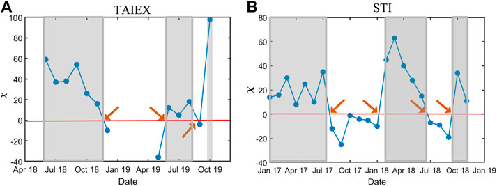
FIGURE 14. The Euler characteristic χ in (A) TAIEX and (B) STI against dates. Each date represents a six-month period in which the correlation matrix was constructed. Besides, different dates are associated with different values of $\mathit{ϵ}$. The gray bands are over the same periods shown in Figure 11 and cover Euler characteristics that are positive.

To show that we indeed observe in the real market data topological changes described in our hypothesis in TDA of Toy Models and Hypothesis on Real Markets Section, we investigated specifically the mini-crash of TAIEX over four time periods. One is just before the crash (Jun 2018 to Nov 2018), two is during the crash (Sep 2018 to Feb 2019) and (Oct 2018 to Mar 2019), and the last is just after the crash (Dec 2018 to May 2019). Here let us point out an important limitation of the Betti numbers, i.e. they do not tell us how big the clusters are. For example, the same set of Betti numbers can describe a collection of clusters that are roughly the same size, some with holes, some without; this market is not close to a crash. Or it can describe a collection of clusters, one of which is a giant cluster containing most of the holes; a market like this is close to a crash. This means that β_n must be supplemented by traditional clustering analysis, where it is easier to see giant clusters, but difficult to understand topological changes.

To this end, we show in Figure 15 the results of average-linkage hierarchical clustering based on the cross-correlation matrices of the four periods. In the first period, we found one giant cluster co-existing with two small clusters. β₀ = 2 for this period is close to the number of clusters we found, confirming our hypothesis that before the crash, we have a growing giant cluster. By tracking which clusters the 671 stocks belong to, we found that in the second period, one of the smaller clusters was absorbed by the giant cluster. In the third period, this membership information revealed the initial stages of the giant cluster breaking up, as it ejected two smaller clusters. For the last period, we now found 12 different clusters, suggesting that we were near the end of the market crash. This fusion and fission phenomenon is in line with the hypothesis we made (see Figure 7D). To tease out subtle topological changes to the giant cluster as the market crash progressed, we looked to changes in the Betti numbers. This is possible because, unlike the use of a single criterion to group stocks in hierarchical clustering, TDA uses multiple criteria to accomplish this task. For example, it is possible for the giant cluster to continue absorbing stocks while it is ejecting others. The overall change in the number of clusters is reflected in β₀, however with β₀ alone we cannot distinguish between $1 – 2=-1$ and $5 – 6=-1$. These two scenarios may be differentiated by the other Betti numbers. Specifically, we found that β₂ changed from $62\to 3\to 4\to 1\to 11\to 44\to 11$ starting from the period (Jun 2018 to Nov 2018) to the period (Dec 2018 to May 2019), implying an initial decrease in the number of 2D holes just before the crash (Figure 7A), becoming 1 in the middle of the crash (Figure 7B), before increasing again just after the crash (Figure 7D).

FIGURE 15

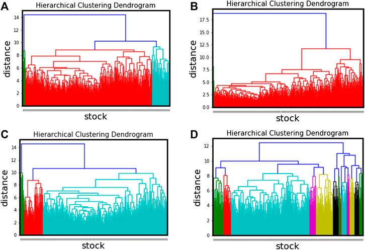
FIGURE 15. The hierarchical clustering dendrogram for four periods in TAIEX, i.e. (A) from Jun 2018 to Nov 2018, (B) Sep 2018 to Feb 2019, (C) Oct 2018 to Mar 2019, and (D) Dec 2018 to May 2019.

We also wanted to check if there are any handle-breaking events during real market crashes. For example, if we start with a torus, the Betti numbers would be ${\beta }_0=1, {\beta }_1=2,$ and ${\beta }_2=1$. If the handle of the torus breaks, the object remaining would be homomorphic to a sphere, which has ${\beta }_0=1, {\beta }_1=0,$ and ${\beta }_2=1$, indicating that handle breaking is a topological change whose signature is $(\Delta {\beta }_0,\Delta {\beta }_1,\Delta {\beta }_2)=(0,-2, 0)$. To track these topological changes, we kept only the giant cluster in each of the period, and recomputed the Betti numbers within these components. During the TAIEX mini-crash, we found the sequence $1\to 4\to 1\to 2$ for β₀, which tells us that the giant cluster for the second period is the least homogeneous. Going beyond β₀, we found the sequence $23\to 61\to 1\to 0$ for β₁. This tells us that the initial giant cluster already contained many irreducible loops, and this number of irreducible loops increased further in the second period as the giant cluster increased in size. By the third period, most of these irreducible loops have disappeared, and by the fourth period, the giant cluster remaining has a simple topological structure. Finally, for β₂, we found the sequence $78\to 29\to 44\to 2$. Specifically, β₂ (the number of enclosed volumes) and β₁ (the number of irreducible loops) can together tell us more about the topology of the simplicial complex. For example, ${\beta }_1=0,{\beta }_2=1$ for a spherical shell, whereas for a torus, ${\beta }_1=2,{\beta }_2=1$. In the first period, we found that ${\beta }_1<{\beta }_2$. This tells us that the giant cluster contains many enclosed volumes that are not holes (because every hole in the simplicial complex must be accompanied by irreducible loops). In the second period, we found instead that ${\beta }_1>{\beta }_2$, and in fact ${\beta }_1\approx 2{\beta }_2$, suggesting that all the enclosed volumes have become holes. The number of handles thus increased from the first period to the second period (although we cannot exclude the possibility that a few of them might have broken, although it is unlikely for many to have broken). From Table 1, we see that the giant cluster broke up most vigorously during the second and third period. Here we see that beyond this fragmentation, the topological changes associated with the second and third periods are very different: in the second period, enclosed volumes became holes, whereas in the third period, the handles of these holes broke and more enclosed volumes emerged. Furthermore, because β₂ was large in the fourth period, the fragmentation products are closer to being spherical shells than they are to solid spheres.

MST, PMFG, and TMFG

In the econophysics literature, we celebrate insights on stock markets obtained using correlation filtering methods. From Mantegna's work [8], we learned to project an arbitrary correlation matrix onto a minimal spanning tree, requiring only N − 1 links when there are N nodes, to visualize the correlational structure of stock markets. However, there is no reason why we should admit only N − 1 links. According to Tumminello et al. [9], the number of non-intersecting links in a graph G with genus g is at most $3(n-2+2g)$, and therefore we may project the correlation matrix onto manifolds with different genus g to keep more links or fewer links. The simplest such projection is onto a sphere (g = 0), or other manifolds with a small genus. The graph that results from projection onto a sphere is planar and is therefore called a planar maximally filtered graph (PMFG). A related method, the triangular maximally filtered graph (TMFG) [10], that checks local planarity but not globally that the genus is zero. This is computationally more efficient and can be parallelized for very large datasets. However, there is no reason to believe that g = 0 is the optimum genus for all correlation matrices computed from stock markets. We believe that genus g implied in Table 1 is optimum because they are computed in an unbiased fashion through the TDA filtration procedure. We can use this optimum genus to systematically improve the efficacy of such information filtering methods.

MST methods have been used to track topological changes during market crashes. To name a few, Onnela et al. [49, 50] investigated the US stocks during the 1987 Black Monday and found that the diameter of the MST decreased during the market crash, so this feature can be used as a universal indicator of market crashes. We ourselves also used the MST of the 10 US Dow Jones economic sectors [51] and the 36 Nikkei industry indices [52] in conjunction with time-series segmentation, to find a core-fringe structure during crizes. In the same spirit, Wilinski et al. [53] and Sienkiewicz et al. [54] investigated market crashes in the Frankfurt Stock exchange (FSE), and the Warsaw Stock Exchange (WSE), and concluded that a two-transition process characterizes market crashes universally. The first transition is from a hierarchical scale-free MST to a superstar-like MST, followed by a second transition to a power-law MST decorated with star-like trees or hubs. In using the MST, they have assumed that loops (β₁) in the networks can be ignored. In this sense, the present is a natural extension to what they have done, where we take a more detailed look into the topological transitions.

Ultimately, informational filtering methods such as MST or PMFG are designed to produce connected graphs and are thus not the best choice for identifying fragmented clusters. To identify these, we can of course use the minimal spanning forest (MSF) [55] or the directed bubble hierarchical tree (DBHT) [56, 57] methods modified from the MST or PMFG. Here, we would like to stress that most clustering approaches are limited to β₀ and β₁, and cannot differentiate topological changes beyond β₁. TDA is promising because it is an elegant extension beyond 0-simplices and 1-simplices, allowing us to unravel subtle topological changes during market crashes.

Outlook and Perspective

Several future directions are possible based on this work. First, in MST, PMFG, and TMFG Section, we mention that the upper bound of the number of links for information filtering methods involving projection to manifolds with genus g is given by $3(n-2+2g)$. The Euler characteristic listed in Tables 1(A, B) can be also be used to calculate the genus g via $\text{χ}=2(1-g)$. With this we are not required to assume a priori that the optimal manifold to project has g = 0 or close to 0. Second, Bubenik [58] had proposed to use persistence landscapes, which is a Banach space that can be converted from persistence diagrams. We then can do statistical averaging of the persistence landscapes, and use the result to design persistence weighted kernels, see for example this very recent work [59]. Persistence weighted kernels can fully maximize the strength of ML algorithms in making stock price predictions. Third, we identified two market crashes in TWSE and several topological phase transitions in SGX.

A pearl of common wisdom that can be gleaned from [47] is that the number of simplices (kth Betti numbers), in general, will peak at k = 6 to k = 8, before dropping to zero at k = 11. More computing resources are required to carry out future works in this direction to test at which k the number of simplices actually peak, and at which k it finally dropped to zero. Also, in Reimann’s work, they investigated directed simplices instead of undirected ones. The former finds applications in educational science, for example [60]. Also, a recent work that applied persistent homology in investigating co-occurrence networks had shown promising results [61].

Conclusion

In this work, we collected daily price data from SGX and TWSE and analyzed them using persistent homology and TDA toolkits. We then made a case for TDA to be employed alongside the other state-of-the-art network embedding techniques including the MST, PMFG, TMFG, in analyzing the topological structures. We were drawn to the application of Persistent Homology (PH) and TDA in complex systems for three reasons: ) PH and TDA are unbiased; ) they scan through a full range of correlation values instead of using only one or two specific values; and ) it is less susceptible to random noises.

We then utilize three toy models to illustrate our hypothesis in Introduction Section, that is “in different market states, their topological features are also changing accordingly, and TDA can be effective in scrutinizing these changes.” We showed in these toy models, including spheres, toruses, and ellipsoids, how χ, the Betti numbers, the barcodes, and persistence diagrams change with topological changes. Also, we use schematic diagrams to illustrate different market states, what the topologies could be like, and argue what their possible Betti numbers and χ’s could be.

Our results revealed unexpected and promising findings in the stock markets. In TWSE, we found a small crash from Sep 2018 to Jan 2019, followed by a larger crash in March 2020, which is due to the COVID-19 pandemic. For these two crashes, we performed three tests using TDA methods. The first test was to quantify a persistence-weakening phenomenon in the barcodes and persistence diagrams. This persistence-weakening phenomenon was also discovered in the SGX, suggesting that it might be universal. However, there were no reported crashes in the SGX for the period studied. To understand this apparent inconsistency, in the second test we calculated the Betti numbers and the Euler characteristic of different 6-months windows in both markets. Our results suggest that market crashes in TAIEX and STI are associated with χ > 0, but the market crash signatures are stronger and have cleaner interpretations in β₀. When we scrutinized the changes to β₀, β₁, and β₂ of the giant cluster over four time periods before, during, and after the TAIEX mini-crash, we found that at the beginning of the crash, the giant cluster has many holes and many more enclosed volumes. As the market crash progressed, these enclosed volumes first became holes, before the handles of these holes broke, to give rise to fragmentation products that were closer to spherical shells than they are to solid spheres. Finally, in the last test, we found the dim-2 persistent entropy decreasing significantly across market crashes. To conclude we found that TDA confirmed most parts of our hypothesis, but also suggested that the topological changes surrounding a market crash are more complex than what we had imagined.

Data Availability Statement

All Python and Matlab scripts are provided, along with instructions on how to use them. These will download the raw data from Yahoo! Finance, perform the necessary computations to give the final results. The files are provided in this link. https://researchdata.ntu.edu.sg/dataset.xhtml?persistentId=doi:10.21979/N9/8XMZGF.

Author Contributions

SC and PT-WY conceived the study, PT-WY collected the data, SC and PT-WY analyzed the data and interpreted the results, SC and PT-WY wrote and reviewed the manuscript.

Funding

This research is supported by a startup grant from the Nanyang Technological University.

Conflict of Interest

The authors declare that the research was conducted in the absence of any commercial or financial relationships that could be construed as a potential conflict of interest.

Acknowledgments

We thank our NTU colleagues Melvin Soh Hwee Jin and Jeric Ho Yew Kee for their assistance in providing advice and solutions to our inquiries on high-performance computing-related issues. P T.W.Y. acknowledges support from ERI@N. We also thank the two anonymous reviewers for their insightful and constructive comments that helped improved our revised manuscript greatly.

Supplementary Material

The Supplementary Material for this article can be found online at: https://www.frontiersin.org/articles/10.3389/fphy.2021.572216/full#supplementary-material.

References

1. Laloux L, Cizeau P, Bouchaud J-P, Potters M. Noise dressing of financial correlation matrices. Phys Rev Lett (1999) 83(7):1467–70. doi:10.1103/PhysRevLett.83.1467

CrossRef Full Text | Google Scholar

2. Plerou V, Gopikrishnan P, Rosenow B, Nunes Amaral LA, Stanley HE. Universal and nonuniversal properties of cross correlations in financial time series. Phys Rev Lett (1999) 83(7):1471–4. doi:10.1103/PhysRevLett.83.1471

CrossRef Full Text | Google Scholar

3. Plerou V, Gopikrishnan P, Rosenow B, Amaral LAN, Stanley HE. A random matrix theory approach to financial cross-correlations. Phys Stat Mech Appl (2000) 287(3-4):374–82. doi:10.1016/s0378-4371(00)00376-9

CrossRef Full Text | Google Scholar

4. Sandoval L, Franca IDP. Correlation of financial markets in times of crisis. Phys Stat Mech Appl (2012) 391(1-2):187–208. doi:10.1016/j.physa.2011.07.023

CrossRef Full Text | Google Scholar

5. Mantegna RN, Stanley HE. Stochastic process with ultraslow convergence to a Gaussian: the truncated Levy flight. Epub 1994/11/28. Phys Rev Lett (1994) 73(22):2946–9. PubMed PMID: 10057243. doi:10.1103/PhysRevLett.73.2946

PubMed Abstract | CrossRef Full Text | Google Scholar

6. Mandelbrot BB, Van Ness JW. Fractional brownian motions, fractional noises and applications. SIAM Rev (1968) 10(4):422–37. doi:10.1137/1010093

CrossRef Full Text | Google Scholar

7. Mandelbrot BB, Fisher AJ, Calvet LE. A multifractal model of asset returns New Haven: Yale University (1997).

8. Mantegna RN. Hierarchical structure in financial markets. The European Physical Journal B (1999) 11(1):193–7. doi:10.1007/s100510050929

CrossRef Full Text | Google Scholar

9. Tumminello M, Aste T, Di Matteo T, Mantegna RN. A tool for filtering information in complex systems. Proc. Natl. Acad. Sci. U.S.A (2005) 102(30):10421–6. doi:10.1073/pnas.0500298102

PubMed Abstract | CrossRef Full Text | Google Scholar

10. Massara GP, Di Matteo T, Aste T. Network filtering for big data: triangulated maximally filtered graph. Journal of Complex Networks (2016) 5(2):161–78. doi:10.1093/comnet/cnw015

CrossRef Full Text | Google Scholar

11. Zomorodian A, Carlsson G. Computing persistent homology. Discrete Comput Geom (2004) 33(2):249–74. doi:10.1007/s00454-004-1146-y

CrossRef Full Text | Google Scholar

12.G Singh, F Mémoli, and GE Carlsson, editors. Topological methods for the analysis of high dimensional data sets and 3d object recognition. Geneva: SPBG (2007).

13.H Edelsbrunner, D Letscher, and A Zomorodian, editors. Topological persistence and simplification. Proceedings 41st annual symposium on foundations of computer science. Redondo Beach, CA, USA, 2000, IEEE (2000). doi:10.1109/SFCS.2000.892133

CrossRef Full Text | Google Scholar

14. Carlsson G. Topology and data. Bull Am Math Soc (2009) 46(2):255–308. doi:10.1090/s0273-0979-09-01249-x

CrossRef Full Text | Google Scholar

15. Hatcher A. Algebraic topology. Cambridge University Press (2002).

16. Edelsbrunner H, Harer J. Computational topology: an introduction. American Mathematical Soc. (2010). doi:10.1007/978-3-540-33259-6_7

CrossRef Full Text

17. Ghrist RW. Elementary applied topology. Seattle: CreateSpace Independent Publishing Platform (2014).

18. Eilenberg S, Steenrod N. Foundations of algebraic topology. Princeton University Press (2015).

19. Munkres JR. Elements of algebraic topology. New York: CRC Press (2018).

CrossRef Full Text

20. Cotton FA. Chemical applications of group theory. John Wiley & Sons (2003).

21. Dresselhaus MS, Dresselhaus G, Jorio A. Group theory: application to the physics of condensed matter. Springer Berlin Heidelberg (2007).

22. Strang G. Linear Algebra and its applications: thomson. Boston: Cengage Learning (2006).

23. Lay DC. Linear algebra and its applications. Addison-Wesley (2012).

24. Barabási A-L. Network science. Cambridge University Press (2016).

25. West DB. Introduction to graph theory. Upper Saddle River: Prentice-Hall (2001).

26. Newman M. Networks: an introduction. Oxford: OUP Oxford (2010).

27. Hausmann J-C. On the Vietoris-Rips complexes and a cohomology theory for metric spaces. Ann Math Stud (1995) 138:175–88. doi:10.1515/9781400882588-013

CrossRef Full Text | Google Scholar

28. Toth CD, O'Rourke J, Goodman JE. Handbook of discrete and computational geometry. Chapman and Hall/CRC (2017).

29.H Edelsbrunner, editor. Smooth surfaces for multi-scale shape representation. International conference on foundations of software technology and theoretical computer science. Springer (1995).

Google Scholar

30. De Silva V, Carlsson GE. Topological estimation using witness complexes. SPBG (2004) 4:157–66. doi:10.2312/SPBG/SPBG04/157-166

CrossRef Full Text | Google Scholar

31. Otter N, Porter MA, Tillmann U, Grindrod P, Harrington HA. A roadmap for the computation of persistent homology. Epub 2017/01/01. EPJ Data Sci (2017) 6(1):17. PubMed PMID: 32025466; PubMed Central PMCID: PMCPMC6979512. doi:10.1140/epjds/s13688-017-0109-5

PubMed Abstract | CrossRef Full Text | Google Scholar

32. Edelsbrunner H, Harer J. Persistent homology-a survey. Contemp Math (2008) 453:257–82.

CrossRef Full Text | Google Scholar

33. Bauer U. Ripser: a lean C++ code for the computation of Vietoris-Rips persistence barcodes. Software (2017). available at. https://github.com/Ripser/ripser (Accessed September 04, 2020).

Google Scholar

34. Carrara N. TDA toolkit (2018). [updated September09/04/2020]. doi:10.5281/zenodo.1436034

CrossRef Full Text

35. Adams H, Tausz A, Vejdemo-Johansson M. Java{P}lex: {A} research software package for persistent (co)homology. In: Hong H, Yap, CK, editors. Proceedings of ICMS. 2014 (2014).

Google Scholar

36. Sornette D. Why stock markets crash: critical events in complex financial systems. New Jersey: Princeton University Press (2017).

CrossRef Full Text

37. Lux T. Herd behaviour, bubbles and crashes. Econ J (1995) 105(431):881–96. doi:10.2307/2235156

CrossRef Full Text | Google Scholar

38. Teh BK, Cheong SA. Cluster fusion-fission dynamics in the Singapore stock exchange. The European Physical Journal B (2015) 88(10):263. doi:10.1140/epjb/e2015-60456-y

CrossRef Full Text | Google Scholar

39. Teh BK, Goo YW, Lian TW, Ong WG, Choi WT, Damodaran M, et al. The Chinese Correction of February 2007: how financial hierarchies change in a market crash. Phys Stat Mech Appl (2015) 424:225–41. doi:10.1016/j.physa.2015.01.024

CrossRef Full Text | Google Scholar

40. Kleinen T, Held H, Petschel-Held G. The potential role of spectral properties in detecting thresholds in the Earth system: application to the thermohaline circulation. Ocean Dynam (2003) 53(2):53–63. doi:10.1007/s10236-002-0023-6

CrossRef Full Text | Google Scholar

41. Scheffer M, Bascompte J, Brock WA, Brovkin V, Carpenter SR, Dakos V, et al. Early-warning signals for critical transitions. Epub 2009/09/04. Nature (2009) 461(7260):53–9. PubMed PMID: 19727193. doi:10.1038/nature08227

PubMed Abstract | CrossRef Full Text | Google Scholar

42. Folke C, Carpenter S, Walker B, Scheffer M, Elmqvist T, Gunderson L, et al. Regime shifts, resilience, and biodiversity in ecosystem management. Annu Rev Ecol Evol Syst (2004) 35(1):557–81. doi:10.1146/annurev.ecolsys.35.021103.105711

CrossRef Full Text | Google Scholar

43. Scheffer M, Carpenter S, Foley JA, Folke C, Walker B. Catastrophic shifts in ecosystems. Epub 2001/10/12. Nature (2001) 413(6856):591–6. PubMed PMID: 11595939. doi:10.1038/35098000

PubMed Abstract | CrossRef Full Text | Google Scholar

44. Rucco M, Castiglione F, Merelli E, Pettini M. Characterisation of the idiotypic immune network through persistent entropy. Proceedings of ECCS Springer proceedings in complexity. Springer (2014). p. 117–28. 2016.

Google Scholar

45. Chintakunta H, Gentimis T, Gonzalez-Diaz R, Jimenez M-J, Krim H. An entropy-based persistence barcodes. Pattern Recogn (2015) 48(2):391–401. doi:10.1016/j.patcog.2014.06.023

CrossRef Full Text | Google Scholar

46. Fan S, Raposo EP, Coutinho-Filho MD, Copelli M, Stam CJ, Douw L. Topological phase transitions in functional brain networks. Epub 2019/10/24. Phys Rev E (2019) 100(3-1):032414, 2019. PubMed PMID: 31640025. doi:10.1103/PhysRevE.100.032414

PubMed Abstract | CrossRef Full Text | Google Scholar

47. Reimann MW, Nolte M, Scolamiero M, Turner K, Perin R, Chindemi G, et al. Cliques of neurons bound into cavities provide a missing link between structure and function. Epub 2017/07/01. Front Comput Neurosci (2017) 11:48, 2017. PubMed PMID: 28659782; PubMed Central PMCID: PMCPMC5467434. doi:10.3389/fncom.2017.00048

PubMed Abstract | CrossRef Full Text | Google Scholar

48. Fan S, da Silva LCB, Coutinho-Filho MD. Topological approach to microcanonical thermodynamics and phase transition of interacting classical spins. J Stat Mech Theor Exp (2017) 2017(1):013202. doi:10.1088/1742-5468/2017/1/013202

CrossRef Full Text | Google Scholar

49. Onnela J-P, Chakraborti A, Kaski K, Kertiész J. Dynamic asset trees and portfolio analysis. The European Physical Journal B-Condensed Matter and Complex Systems (2002) 30(3):285–8.

CrossRef Full Text | Google Scholar

50. Onnela J-P, Chakraborti A, Kaski K, Kertesz J. Dynamic asset trees and Black Monday. Phys Stat Mech Appl (2003) 324(1-2):247–52.

CrossRef Full Text | Google Scholar

51. Zhang Y, Lee GHT, Wong JC, Kok JL, Prusty M, Cheong SA. Will the US economy recover in 2010? A minimal spanning tree study. Phys Stat Mech Appl (2011) 390(11):2020–50.

CrossRef Full Text | Google Scholar

52. Cheong SA, Fornia RP, Lee GHT, Kok JL, Yim WS, Xu DY, et al. The Japanese economy in crises: a time series segmentation study. Economics: the Open-Access. Open-Assessment E-Journal (2012) 6(2012-5):1–81.

CrossRef Full Text | Google Scholar

53. Wiliński M, Sienkiewicz A, Gubiec T, Kutner R, Struzik Z. Structural and topological phase transitions on the German Stock Exchange. Phys Stat Mech Appl (2013) 392(23):5963–73.

Google Scholar

54. Sienkiewicz A, Gubiec T, Kutner R, Struzik ZR. Dynamic structural and topological phase transitions on the Warsaw Stock Exchange: A phenomenological approach. arXiv preprint arXiv:13016506 (2013).

55. Di Gesù V, Sacco B. Some statistical properties of the minimum spanning forest. Pattern Recognition (1983) 16(5):525–31.

Google Scholar

56. Song W-M, Di Matteo T, Aste T. Hierarchical information clustering by means of topologically embedded graphs. PloS One (2012) 7(3):e31929.

PubMed Abstract | CrossRef Full Text | Google Scholar

57. Musmeci N, Aste T, Di Matteo T. Relation between financial market structure and the real economy: comparison between clustering methods. PloS One (2015) 10(3):e0116201.

PubMed Abstract | CrossRef Full Text | Google Scholar

58. Bubenik P. Statistical topological data analysis using persistence landscapes. J Mach Learn Res (2015) 16(1):77–102. doi:10.5555/2789272.2789275

CrossRef Full Text | Google Scholar

59.G Kusano, Y Hiraoka, and K Fukumizu, editors. Persistence weighted Gaussian kernel for topological data analysis. New York: International Conference on Machine Learning (2016).

Google Scholar

60. Goh WP, Kwek D, Hogan D, Cheong SA. Complex network analysis of teaching practices. EPJ Data Science (2014) 3(1):1–16. doi:10.1140/epjds/s13688-014-0034-9

CrossRef Full Text | Google Scholar

61. Salnikov V, Cassese D, Lambiotte R, Jones NS. Co-occurrence simplicial complexes in mathematics: identifying the holes of knowledge. Epub 2018/01/01. Appl Netw Sci (2018) 3(1):37. PubMed PMID: 30839828; PubMed Central PMCID: PMCPMC6214324. doi:10.1007/s41109-018-0074-3

PubMed Abstract | CrossRef Full Text | Google Scholar