Construction of C1 Rational Bi-Quartic Spline With Positivity-Preserving Interpolation: Numerical Results and Analysis

From the observed datasets, we should be able to produce curve surfaces that have the same characteristics as the original datasets. For instance, if the given data are positive, then the resulting curve or surface must be positive on entire given intervals, i.e., everywhere. In this study, a new partial blended rational bi-quartic spline with C¹ continuity is constructed through the partially blended scheme. This rational spline is defined on four corners of the rectangular meshes. The sufficient condition for the positivity of rational bi-quartic spline is derived on four boundary curve networks. There are eight free parameters that can be used for shape modification. The first-order partial derivatives are estimated by using numerical techniques. We also show that the proposed scheme is local quadratic reproducing such that it can exactly reproduce the quadratic surface. We test the proposed scheme to interpolate various types of positive surface data. Based on statistical indicators such as the root mean square error (RMSE) and coefficient of determination (R²), we found that the proposed scheme is on par with some established schemes. In fact, it requires less CPU times (in seconds) to generate the interpolating surface on rectangular meshes. Furthermore, by combining the statistical indicators’ result and graphically visualizing the test functions, the proposed method has the capability to reconstruct very comparable smoothing interpolating positive surfaces compared to some existing schemes. This finding is significant in producing a better interpolating surface for computer graphics applications since the proposed scheme has a smaller error compared with existing schemes.

Introduction

Computer-aided geometric design (CAGD) provides the mathematical basis when dealing with geometric datasets. The term “CAGD” was coined by Barnhill and Riesenfeld in 1974 [1–5]. One of the main tools in CAGD is a spline function. The spline function was introduced by Schoenberg in 1967 for application in statistics. Since then, the spline has been used extensively in shape designing especially in car industries, in the design of airplane fuselages and wings at Boeing Company, as well as in the development of cartoon movies. General Motors developed its first computer-aided design/computer-aided manufacturing (CAD/CAM) system called DAC-I by utilizing the spline curve and surface techniques initiated by de Boor and Gordon [5]. Furthermore, in some applications, such as data visualization, there is a need to reconstruct the curve or surface for the data collected from the measurement or experimental laboratory. This task can be achieved by using interpolation or approximation schemes.

Shape-preserving interpolation is an important topic in CAGD that can be used to preserve the geometric shape of the dataset such as positivity, convexity, and monotonicity. For instance, given positive data, then the final interpolating curve or surface must be positive everywhere. Any negativity is meaningless and unacceptable. Some examples of positive data are the amount of gas discharge during the experiment (Brodlie and Butt [6], Butt and Brodlie [7], Brodlie et al. [8], Sarfraz et al. [9]). Meanwhile, monotonicity-preserving concerns about preserving the monotone datasets, i.e., either monotonically increasing or monotonically decreasing. For instance, the approximation of couples and quasi-couples in statistics and the empirical option model in finance are always involving monotone datasets [10]. The blood uric acid in patients suffering from gout is also an example of monotone data. Meanwhile, convexity always arises in finance and engineering-based problems such as the optimal control, non-linear programming, and parameter estimation problems.

In general, the standard cubic Hermite polynomial and cubic spline interpolation functions are unable to produce the interpolating curve or surface with shape-preserving properties. Therefore, to cater this weakness, many researchers have proposed several methods for shape-preserving approximation and interpolation. One of the simplest ways is to use rational splines in many different forms such as cubic/cubic, cubic/quadratic, cubic/linear, and quartic/quadratic. Those schemes provided more design parameters which can be used to modify the interpolating curves or surfaces. In the next paragraphs, we provide some literature review on positivity-preserving interpolation schemes.

The modified quadratic Shepard (MQS) method has been used widely for visualization of scattered data. For example, Asim et al. [11, 12] improved the original MQS method for positivity-preserving on scattered datasets. Their strategy is to reduce the deviation from the original shape while at the same time preserving positivity in the sense of least square. Brodlie et al. [8] constructed the MQS method to interpolate scattered data of any dimensionality. Their scheme preserves the positivity of the data for curves or surfaces by forcing the quadratic basis functions to be positive. They also extended the method to handle modeling other types of constraints such as the lower bound of 0 and upper bound of 1 and generalized the constraint to any arbitrary functions as lower and upper bounds. But from the numerical results, they indicated that their schemes have 10% error bound associated with the data values. Wu et al. [13] discussed about positivity-preserving for curve and surface approximation and interpolation by using compactly supported radial basis functions (CSRBFs). To preserve the positivity of data, the optimization problem needs to be solved. In [14, 15], the multi-quadric (MQ) function has been used as the quasi-interpolation operator and the CSRBFs are used to construct the interpolation function that preserves the monotonicity and convexity of planar datasets.

Most shape-preserving surface interpolation methods are constructed by extending the work of Casciola and Romani [16]. Nowadays, their schemes are known as partially blended rational bi-cubic functions. Brodlie and Butt [6] constructed the piecewise cubic Hermite interpolant with $C^1$continuity to preserve positivity, monotonicity, and convexity, respectively. Their schemes required one or two extra knots to be inserted in the interval where shape violation exists without needs for derivative modification. However, this technique will increase the total number of data points, and indeed, the computation times will be increased.

Brodlie et al. [8] extended the Butt and Brodlie [7] idea to construct the positivity-preserving scheme of positive surface data over a rectangular grid. The sufficient conditions on first partial derivatives and twist values are derived where the obtained values will be projected to the valid interval through the efficient knot insertion algorithm. However, their scheme has increased unnecessary computation time.

Schmidt and Hess [17, 18] derived the necessary and sufficient conditions for the positivity of rational quadratic splines and for the positivity of cubic spline interpolation on intervals. Schmidt [19] described the positive, monotone, and $S$-convex surface interpolation for data arranged on rectangular grids. The $C^1$ rational quadratic spline has been used, and the necessary conditions for positivity, monotonicity, and $S$-convex surface are derived. However, no numerical results were presented. Hussain et al. [20] constructed $C^0$ shape-preserving surface schemes for 3D positive and convex surface data. The rational bi-quadratic function with eight parameters was used to construct the positive and monotone rational interpolant. But their scheme was unable to produce smooth surfaces as well as no free parameters to alter the final resulting interpolating surfaces. Chan and Ong [21] described a local scheme for range-restricted scattered data interpolation by using cubic triangular Bézier patches. The piecewise interpolating surface is obtained through a convex combination of three cubic Bézier triangular patches. The sufficient conditions for the non-negativity of a cubic Bézier triangle on the Bézier ordinates were derived with respect to a lower bound. The gradients (first-order partial derivatives) at the data sites are modified if necessary, to ensure that the non-negativity conditions are fulfilled. Luo and Peng [22] described the $C^1$ rational spline as a piecewise rational convex combination of three cubic Bézier triangular patches sharing the same boundary Bézier ordinates. The sufficient conditions for non-negativity were derived on the boundary Bézier ordinates of the adjacent triangle and the normal derivatives at the data points. If in any triangular patch non-negativity was lost, then the gradients at the data points and normal derivatives at the edge knots will be modified to ensure positivity is preserved. Indeed, their main scheme also requires the modification of the first-order partial derivative and the normal derivatives if shape violation is found.

Piah et al. [23] improved the lower bound of Bézier ordinates obtained in the work of Chan and Ong [21] by proposing an alternative scheme which is simpler and has more relaxed conditions of positivity. The new lower bound for Bézier ordinates can become infinitely smaller compared to the lower bound of Bézier ordinates in [21]. Some numerical results were presented to show the capability of the alternative scheme. The main drawback of their scheme is that the actual first-order partial derivative needs to be adjusted if positivity on each triangular patch is violated. Hussain and Hussain [24] constructed positive scattered data interpolation by using a rational cubic spline defined by the side-vertex scheme.

Saaban et al. [25] constructed the positivity-preserving scheme by using quintic triangular Bézier patches. The surface is constructed by using a convex combination comprising of three local quintic triangular Bézier patches. They implemented their proposed method by using rainfall data collected at various meteorology stations in West (Peninsular) Malaysia.

Hussain et al. [26, 27] extended the application of rational quartic spline given by Wang and Tan [28] to preserve positivity, constrained data, and convexity. The data-dependent sufficient conditions for the rational interpolant to satisfy the shape-preserving properties are derived. It was proved by Harim et al. [29] that their sufficient conditions may not successfully produce positive and convex interpolating curves on entire given intervals.

Liu et al. [30] described a new bivariate rational quartic spline (quartic/quadratic) for positivity- and monotonicity-preserving interpolation. The rational bi-quartic spline has four parameters, and the sufficient conditions for positivity and monotonicity are derived on all parameters. Thus, there is no free parameter for shape modification. They have compared the performance of their schemes against that of Hussain and Sarfraz’s [31] for positivity-preserving interpolation. No error measurement is given to show the superiority of the proposed scheme. Han [32, 33] discussed the rational quartic spline with a quadratic denominator. Harim et al. [29, 34, 35] constructed a new rational quartic spline (quartic/quadratic) with three parameters for shape modification. Karim et al. [31, 36, 37] discussed the positivity-preserving interpolation and constrained surface modeling by using rational bi-cubic spline interpolation with 12 parameters. Qin et al. [38] proposed a new method to derive the sufficient condition for the positivity of rational bi-cubic spline interpolation. However, their method requires extra computation time.

In this section, we have given a comprehensive review on the existing schemes of positivity-preserving interpolation. Table 1 summarizes the comparison of various shape-preserving interpolation schemes related to our studies.

TABLE 1

TABLE 1. Comparison of shape-preserving schemes.

From Table 1, we have come out with our main objectives of the study. There are three main objectives given as follows:

1) We extend the univariate rational quartic spline with three parameters from Harim et al. [34] to the bivariate rational quartic spline interpolation. We employ the partially blended scheme initiated by Casciola and Romani [16]. There are three free parameters on each boundary of the rectangular meshes. This will give 12 parameters that can be used to control the shape of the interpolating surface.

2) To derive the sufficient condition for the positivity of the rational bi-quartic spline on each boundary, we also derive the quadratic polynomial reproducing.

3) Finally, to compare the performance between the proposed scheme for positivity-preserving interpolation and some established schemes such as Abbas et al. [50] and Karim et al. [36], the root mean square error (RMSE) and coefficient of determination (R²) are used as statistical goodness-of-fit measurements [53].

Furthermore, we identified several advantages of the proposed partially blended rational bi-quartic spline interpolation for positivity-preserving:

1) There are 12 parameters in the description of the rational bi-quartic spline, and eight are free parameters for shape modification. Meanwhile, Hussain and Ali [37], Hussain and Hussain [40], Tian et al. [41], and Sarfraz et al. [9] schemes have no free parameters for shape modification.

2) Unlike existing schemes such as Karim et al. [36], Abbas et al. [50, 51], Hussain and Ali [37], Hussain and Hussain [40], Tian et al. [41], and Sarfraz et al. [9], the proposed scheme is local quadratic reproducing. This is one of the main novelties of the proposed scheme.

3) Based on statistical indicators, i.e., root mean square error (RMSE) and coefficient of determination (R²), the proposed partially blended rational bi-quartic spline is the best compared with the works of Abbas et al. [50] and Karim et al. [36]. In fact, the proposed scheme has a smaller RMSE error and higher R² compared with Brodlie et al.’s scheme [7].

4) Furthermore, the proposed scheme is direct and not involving any iterative scheme via the subdivision scheme as discussed by Ashraf et al. [43].

The remainder of this paper is organized as follows. Materials and Methods is devoted to materials and methods used in this study. This includes the method to estimate first derivatives using the arithmetic mean method (AMM) and geometric mean method (GMM), a review on the rational quartic spline, the derivation of the rational bi-quartic spline, and local control and quadratic reproducing properties. Meanwhile, Positivity-Preserving Interpolation discusses the construction of positive rational bi-quartic spline interpolation on each boundary curve network. Furthermore, an efficient algorithm is presented in detail. Results and Discussion is devoted to the results obtained and discussion. Conclusion gives the concluding remarks.

Materials and Methods

Derivative Estimation

In most applications, the first derivative needs to be estimated by using some numerical methods. Three common methods are the arithmetic mean method (AMM), geometric mean method (GMM), and harmonic mean method (HMM) [54].

Arithmetic Mean Method

Given scalar datasets $\left\{\left(x_i,f_i\right):i=\mathrm{0,1},\mathrm{...},n\right\}$ where$x_0<x_1<\mathrm{...}<x_n$. Let the step size $h_i=x_{i+1}-x_i$ and the gradient ${\Delta }_i=\frac{f_{i+1}-f_i}{h_i}$, $i=\mathrm{0,1},\mathrm{...},n-1$. The first derivatives $d_i$ at the data point $x_i,i=\mathrm{0,1},\mathrm{...},n$, can be estimated as follows.

At both end points$x_0$ and $x_n$, the first derivatives are [54]

$d_0={\Delta }_0+\left({\Delta }_0-{\Delta }_1\right)\left(\frac{h_0}{h_0+h_1}\right),(1)$

$d_n={\Delta }_{n-1}+\left({\Delta }_{n-1}-{\Delta }_{n-2}\right)\left(\frac{h_{n-1}}{h_{n-1}+h_{n-2}}\right).(2)$

Meanwhile, at the interior points, $x_i,i=\mathrm{1,2},\mathrm{...},n-1$, the values of $d_i$ are estimated using the following formula:

$d_i=\frac{h_{i-1}{\Delta }_i+h_i{\Delta }_{i-1}}{h_{i-1}+h_i}.(3)$

Formulas in Equations (1)–(3) can be extended to 3D data as follows.

Given 3D datasets $\left\{\left(x_i,y_j,F_{i,j}\right):i=\mathrm{0,1},\mathrm{...},n; j=\mathrm{0,1},\mathrm{...},m\right\}$. Let $h_i=x_{i+1}-x_i, {\widehat{h}}_j=y_{j+1}-y_j,$${\Delta }_{i,j}=\frac{f_{i+1}-f_i}{h_i}$, and ${\widehat{\Delta }}_{i,j}=\frac{f_{i,j+1}-f_{i,j}}{{\widehat{h}}_j}$. The first partial derivatives are given as follows.

The first partial derivative in the $x$direction is given as

$F_{0,j}^x={\Delta }_{0,j}+\left({\Delta }_{0,j}-{\Delta }_{1,j}\right)\frac{h_1}{\left(h_1+h_2\right)},(4)$

$F_{n,j}^x={\Delta }_{n-1,j}+\left({\Delta }_{n-1,j}-{\Delta }_{n-2,j}\right)\frac{h_{n-1}}{\left(h_{n-1}+h_{n-2}\right)},(5)$

$F_{i,j}^x=\frac{{\Delta }_{i,j}+{\Delta }_{i-1,j}}{2}(6)$

for $i=\mathrm{1,2},\mathrm{...},n-1, j=\mathrm{0,1},\mathrm{...},m$.

The first partial derivative in the $y$ direction is given as

$F_{i,0}^y={\widehat{\Delta }}_{i,0}+\left({\widehat{\Delta }}_{i,0}-{\widehat{\Delta }}_{i,1}\right)\frac{{\widehat{h}}_1}{\left({\widehat{h}}_1+{\widehat{h}}_2\right)},(7)$

$F_{i,m}^y={\widehat{\Delta }}_{i,m-1}+\left({\widehat{\Delta }}_{i,m-1}-{\widehat{\Delta }}_{i,m-2}\right)\frac{{\widehat{h}}_{m-1}}{\left({\widehat{h}}_{m-1}+{\widehat{h}}_{m-2}\right)},(8)$

$F_{i,j}^y=\frac{{\widehat{\Delta }}_{i,j}+{\widehat{\Delta }}_{i,j-1}}{2}(9)$

for $i=\mathrm{0,1,2},\mathrm{...},n, j=\mathrm{1,2},\mathrm{...},m-1$. Meanwhile, the twists (mixed derivative) at the interior points can be estimated by

$F_{i,j}^{xy}=\frac{F_{i+1,j}^y-F_{i-1,j}^y}{h_{i-1}+h_i}+\frac{F_{i,j+1}^x-F_{i,j-1}^x}{{\widehat{h}}_{j-1}+{\widehat{h}}_j},i=\mathrm{1,2},\mathrm{...},n-1, j=\mathrm{1,2},\mathrm{...},m-1.(10)$

Geometric Mean Method

The first derivatives also can be calculated by using the GMM. Given 2D data $\left\{\left(x_i,f_i\right):i=\mathrm{0,1},\mathrm{...},n\right\}$, at the end points$x_0$ and $x_n$, the first derivatives are given as

$d_0=\{\begin{array}{cc}0& if {\text{Δ}}_0=0 or {\text{Δ}}_{\mathrm{2,0}}=0 \\ {\Delta }_0^{\left(1+\frac{h_0}{h_1}\right)}{\Delta }_{\mathrm{2,0}}^{\left(-\frac{h_0}{h_1}\right)}& otherwise,\end{array}(11)$

with ${\Delta }_{\mathrm{2,0}}=\frac{f_2-f_0}{x_2-x_0},$ and

$d_n=\{\begin{array}{cc}0& if {\text{Δ}}_{n-1}=0 or {\text{Δ}}_{n,n-2}=0 \\ {\Delta }_{n-1}^{\left(1+\frac{h_{n-1}}{h_{n-2}}\right)}{\Delta }_{n,n-2}^{\left(-\frac{h_{n-1}}{h_{n-2}}\right)}& otherwise,\end{array}(12)$

with ${\Delta }_{n,n-2}=\frac{f_n-f_{n-2}}{x_n-x_{n-2}}.$

Meanwhile, at interior points, $x_i,i=\mathrm{1,2},\mathrm{...},n-1$, the values of $d_i$ are estimated by

$d_i={\Delta }_{i-1}^{\left(\frac{h_i}{h_{i-1}+h_i}\right)}{\Delta }_i^{\left(\frac{h_{i-1}}{h_{i-1}+h_i}\right)}.(13)$

The advantages of using this choice are the values of $d_i$ are always positive. This method is suitable for monotonically increasing data.

Rational Quartic Spline Interpolation

Given scalar datasets $\left\{(x_I,f_i),i=\mathrm{0,1,2},\mathrm{..}n\right\}$ where $x_0<x_1<\mathrm{...}<x_n$ and the first derivative$d_i$, at the respective point. Then, the RQS scheme with three shape control parameters${\alpha }_i>0,{\beta }_i>0$, and${\gamma }_i\ge 0$on the interval is given by [29, 34, 35]

$\text{S}\left(\text{x}\right)=\frac{{\text{P}}_{\text{i}}\left(\text{θ}\right)}{{\text{Q}}_{\text{i}}\left(\text{θ}\right)},(14)$

where

$\begin{array}{c}{P}_i\left(\theta \right)={\left(1-\theta \right)}^4{\alpha }_i{f}_i+{\left(1-\theta \right)}^3\theta A_i+{\left(1-\theta \right)}^2{\theta }^2{B}_i+\left(1-\theta \right){\theta }^3{C}_i+{\theta }^4{\beta }_i{f}_{i+1}\\ Q_i\left(\theta \right)={\alpha }_i{\left(1-\theta \right)}^2+{\gamma }_i\left(1-\theta \right)\theta +{\beta }_i{\theta }^2\end{array},$

with $h_i=x_{i+1}-x_i$,${\Delta }_i=\frac{f_{i+1}-f_i}{h_i}$, and $\theta =\frac{x-x_i}{h_i}$.

The RQS scheme defined in Eq. 14 gives the C¹ continuity at the knots and satisfies the following conditions:

$\begin{array}{cc}S\left(x_i\right)=f_i,& S\left(x_{i+1}\right)=f_{i+1},\\ S^{\left(1\right)}\left(x_i\right)=d_i,& S^{\left(1\right)}\left(x_{i+1}\right)=d_{i+1}.\end{array}(15)$

From Eq. 15 and after some derivations, the unknown ${\text{A}}_{\text{i}}, {\text{B}}_{\text{i}}$, and $C_i$ are given as [34]

$\begin{array}{l}{A}_i=\left(2{\alpha }_i+{\gamma }_i\right)f_i+{\alpha }_i{h}_i{d}_i,\\ B_i=\left({\alpha }_i+{\gamma }_i\right)f_{i+1}+\left({\beta }_i+{\gamma }_i\right)f_i,\\ C_i=\left(2{\alpha }_i+{\gamma }_i\right)f_{i+1}+{\beta }_i{h}_i{d}_{i+1}.\end{array}(16)$

Partially Blended Rational Bi-Quartic Spline Interpolation

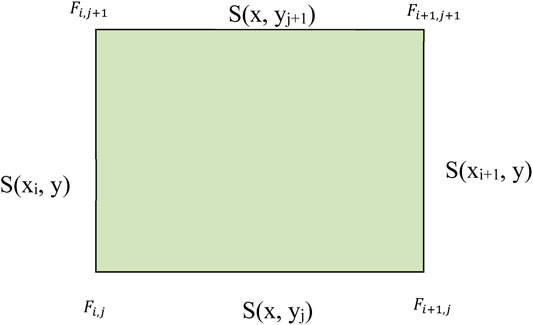
We construct a new rational bi-quartic spline based on the partially blended scheme of Casciola and Romani [16]. There are four curve networks on each edge of the rectangular domain. Figure 1 shows the arrangement of the partially blended rational bi-quartic spline interpolation on a rectangular domain.

FIGURE 1

FIGURE 1. Rational bi-quartic spline defined on a rectangular patch boundary.

Let the function $S\left(x,y\right)$ be arranged over a rectangular domain $\Omega =\left[a,b\right]\times \left[c,d\right]$. The partition of the intervals $\left[a,b\right]$ and $\left[c,d\right]$ is defined as $\pi :a=x_0<x_1<\cdots <x_n=b$ and $\overline{\pi }:c=y_0<y_1<\cdots <y_m=d.$ Let $F_{i,j}$, $F_{i,j}^x$, and $F_{i,j}^y$ indicate the data values and the first partial derivatives with respect to $x$ and $y$ at the node $\left(x_i,y_j\right)$. The partially blended rational bi-quartic function over each rectangle $\left[x_i,x_{i+1}\right]\times \left[y_j,y_{j+1}\right],i=\mathrm{0,1},\mathrm{...},n-1; j=\mathrm{0,1},\mathrm{...},m-1$, is defined as follows:

$S \left(x,y\right)=-AF{B}^{ T},(17)$

with

$\begin{array}{c}F=\left(\begin{array}{ccc}0& S\left(x,y_j\right)& S\left(x,y_{j+1}\right)\\ S\left(x_i,y\right)& S\left(x_i,y_j\right)& S\left(x_i,y_{j+1}\right)\\ S\left(x_{i+1},y\right)& S\left(x_{i+1},y_j\right)& S\left(x_{i+1},y_{j+1}\right)\end{array}\right),\\ A=\left[\begin{array}{ccc}-1& a_0\left(\theta \right)& a_1\left(\theta \right)\end{array}\right],\\ B=\left[\begin{array}{ccc}-1& b_0\left(\phi \right)& b_1\left(\phi \right)\end{array}\right],\end{array}$

where

$\begin{array}{c}{a}_0\left(\theta \right)={\left(1-\theta \right)}^2\left(1+2\theta \right),a_1\left(\theta \right)={\theta }^2\left(3-2\theta \right),b_0\left(\phi \right)={\left(1-\phi \right)}^2\left(1+2\phi \right),b_1\left(\phi \right)={\phi }^2\left(3-2\phi \right),\\ \theta =\frac{x-x_i}{h_i}, \phi =\frac{y-y_j}{{\widehat{h}}_j}, \end{array}$

and

$h_i=x_{i+1}-x_i, {\widehat{h}}_j=y_{j+1}-y_j.$

$S\left(x,y_j\right),S\left(x,y_{j+1}\right),S\left(x_i,y\right)$, and $S\left(x_{i+1},y\right)$ are rational quartic functions defined in Equations (18)–(21) arranged on the edges of the rectangular domain $\left[x_i,x_{i+1}\right]\times \left[y_j,y_{j+1}\right],i=\mathrm{0,1},\mathrm{...},n-1; j=\mathrm{0,1},\mathrm{...},m-1$ (see Figure 1). They are defined as

$S\left(x,y_j\right)=\frac{{{\displaystyle \sum }}_{i=0}^4{\left(1-\theta \right)}^{4-i}{\theta }^i{A}_i}{q_1\left(\theta \right)},(18)$

with

$\begin{array}{c}{A}_0={\alpha }_{i,j}{F}_{i,j}, {\alpha }_{i,j}>0,A_1=\left(2{\alpha }_{i,j}+{\gamma }_{i,j}\right)F_{i,j}+{\alpha }_{i,j}{h}_i{F}_{i,j}^x, {\beta }_{i,j}>0,{\gamma }_{i,j}\ge 0 ,\\ A_2=\left({\alpha }_{i,j}+{\gamma }_{i,j}\right)F_{i+1,j}+\left({\beta }_{i,j}+{\gamma }_{i,j}\right)F_{i,j},A_3=\left(2{\beta }_{i,j}+{\gamma }_{i,j}\right)F_{i+1,j}-{\beta }_{i,j}{h}_i{F}_{i+1,j}^x,A_4={\beta }_{i,j}{F}_{i+1,j},\\ q_1\left(\theta \right)={\left(1-\theta \right)}^2{\alpha }_{i,j}+{\gamma }_{i,j}\theta \left(1-\theta \right)+{\theta }^2{\beta }_{i,j};\\ S\left(x,y_{j+1}\right)=\frac{{{\displaystyle \sum }}_{i=0}^4{\left(1-\theta \right)}^{3-i}{\theta }^i{B}_i}{q_2\left(\theta \right)}\end{array},(19)$

with

$\begin{array}{c}{B}_0={\alpha }_{i,j+1}{F}_{i,j+1}, {\alpha }_{i,j+1}>0,B_1=\left(2{\alpha }_{i,j+1}+{\gamma }_{i,j+1}\right)F_{i,j+1}+{\alpha }_{i,j+1}{h}_i{F}_{i,j+1}^x,{\beta }_{i,j+1}>0, {\gamma }_{i,j+1}\ge 0\\ A{B}_2=\left({\alpha }_{i,j+1}+{\gamma }_{i,j+1}\right)F_{i+1,j+1}+\left({\beta }_{i,j+1}+{\gamma }_{i,j+1}\right)F_{i,j+1},B_3=\left(2{\beta }_{i,j+1}+{\gamma }_{i,j+1}\right)F_{i+1,j+1}-{\beta }_{i,j+1}{h}_i{F}_{i+1,j+1}^x,B_4={\beta }_{i,j}F\\ q_2\left(\theta \right)={\left(1-\theta \right)}^2{\alpha }_{i,j+1}+{\gamma }_{i,j+1}\theta \left(1-\theta \right)+{\theta }^2{\beta }_{i,j+1};\\ S\left(x_i,y\right)=\frac{{{\displaystyle \sum }}_{i=0}^4{\left(1-\phi \right)}^{3-i}{\phi }^i{C}_i}{q_3\left(\phi \right)}\end{array},(20)$

with

$\begin{array}{c}\begin{array}{cc}{C}_0={\widehat{\alpha }}_{i,j}{F}_{i,j},& {\widehat{\alpha }}_{i,j}>0\end{array},C_1=\left(2{\widehat{\alpha }}_{i,j}+{\widehat{\gamma }}_{i,j}\right)F_{i,j}+{\widehat{\alpha }}_{i,j}{\widehat{h}}_j{F}_{i,j}^y, {\widehat{\beta }}_{i,j}>0, {\widehat{\gamma }}_{i,j}\ge 0 ,\\ C_2=\left({\widehat{\alpha }}_{i,j}+{\widehat{\gamma }}_{i,j}\right)F_{i,j+1}+\left({\widehat{\beta }}_{i,j}+{\widehat{\gamma }}_{i,j}\right)F_{i,j},C_3=\left(2{\widehat{\beta }}_{i,j}+{\widehat{\gamma }}_{i,j}\right)F_{i,j+1}-{\widehat{\beta }}_{i,j}{\widehat{h}}_j{F}_{i,j+1}^y,C_4={\widehat{\beta }}_{i,j}{F}_{i,j+1},\\ q_3\left(\phi \right)={\left(1-\phi \right)}^2{\widehat{\alpha }}_{i,j}+{\widehat{\gamma }}_{i,j}\phi \left(1-\phi \right)+{\phi }^2{\widehat{\beta }}_{i,j}\\ S\left(x_{i+1},y\right)=\frac{{{\displaystyle \sum }}_{i=0}^4{\left(1-\phi \right)}^{3-i}{\phi }^i{D}_i}{q_4\left(\phi \right)}\end{array}(21)$

with

$\begin{array}{c}{D}_0={\widehat{\alpha }}_{i+1,j}{F}_{i+1,j}, {\widehat{\alpha }}_{i+1,j}>0,D_1=\left(2{\widehat{\alpha }}_{i+1,j}+{\widehat{\gamma }}_{i+1,j}\right)F_{i+1,j}+{\widehat{\alpha }}_{i+1,j}{\widehat{h}}_j{F}_{i+1,j}^y, {\widehat{\beta }}_{i+1,j}>0, {\widehat{\gamma }}_{i+1,j}\ge 0,\\ D_2=\left({\widehat{\alpha }}_{i+1,j}+{\widehat{\gamma }}_{i+1,j}\right)F_{i+1,j+1}+\left({\widehat{\beta }}_{i+1,j}+{\widehat{\gamma }}_{i+1,j}\right)F_{i+1,j},D_3=\left(2{\widehat{\beta }}_{i+1,j}+{\widehat{\gamma }}_{i+1,j}\right)F_{i+1,j+1}-{\widehat{\beta }}_{i+1,j}{\widehat{h}}_j{F}_{i+1,j+1}^y,\\ q_4\left(\phi \right)={\left(1-\phi \right)}^2{\widehat{\alpha }}_{i+1,j}+{\widehat{\gamma }}_{i+1,j}\phi \left(1-\phi \right)+{\phi }^2{\widehat{\beta }}_{i+1,j}.\end{array}$

The partial derivatives $F_{i,j}^x$ and $F_{i,j}^y$ are estimated by using the AMM given in Equations (4)–(10).

Local Control Shape Property Analysis

The proposed rational bi-quartic spline defined by Eq. 17 has local control properties. Some observations can be made as follows:

1) The proposed scheme is symmetrical, i.e., the surface can be constructed either in x and y directions or in y and x directions. This is one of the main properties in CAGD.

2) When the parameters ${\alpha }_{i,j}= {\alpha }_{i,j+1}= {\beta }_{i,j}={\beta }_{i,j+1}=1, {\widehat{\alpha }}_{i,j}= {\widehat{\alpha }}_{i+1,j}= {\widehat{\beta }}_{i,j}= {\widehat{\beta }}_{i+1,j}=1$, and ${\gamma }_{i,j}={\gamma }_{i,j+1}={\widehat{\gamma }}_{i,j}={\widehat{\gamma }}_{i+1,j}=2$, the partially blended rational bi-quartic spline in Eq. 17 reduced to a standard bi-quartic polynomial spline. Usually, in this case, the resulting interpolating surface is not shape-preserving.

3) When ${\gamma }_{i,j}\to \infty$or ${\alpha }_{i,j},{\beta }_{i,j}\to 0,$the partially blended rational bi-quartic spline defined by Eq. 17 is reduced to a bilinear surface, i.e., flat surface, since all four curve networks are reduced to a straight line (see [34]):

$\underset{{\gamma }_{i\to \infty }}{\lim }S\left(x,y_j\right)=\underset{{\alpha }_{i,{\beta }_i\to 0}}{\lim }S\left(x,y_j\right)=\left(1-\theta \right)F_{i,j}+\theta F_{i+1,j}.(22)$

• Similarly, we can obtain the following observations:

$\underset{{\gamma }_{i,j+1\to \infty }}{\lim }S\left(x,y_{j+1}\right)=\underset{{\alpha }_{i,j+1,{\beta }_{i,j+1}\to 0}}{\lim }S\left(x,y_{j+1}\right)=\left(1-\theta \right)F_{i,j+1}+\theta F_{i+1,j+1},(23)$

$\underset{{\widehat{\gamma }}_{i,j}\to \infty }{\lim }S\left(x_i,y\right)=\underset{{\widehat{\alpha }}_{i,j},{\widehat{\beta }}_{i,j}\to 0}{\lim }S\left(x_i,y\right)=\left(1-\phi \right)F_{i,j}+\phi F_{i,j+1},(24)$

$\underset{{\widehat{\gamma }}_{i+1,j}\to \infty }{\lim }S\left(x_{i+1},y\right)=\underset{{\widehat{\alpha }}_{i+1,j},{\widehat{\beta }}_{i+1,j}\to 0}{\lim }S\left(x_{i+1},y\right)=\left(1-\phi \right)F_{i+1,j}+\phi F_{i+1,j+1}.(25)$

Based on Equations (22)–(25), we conclude that the final interpolating surface is a bilinear surface.

Theorem 1. The partially blended rational bi-quartic spline interpolation defined in Eq. 17 is C¹ continuous everywhere provided that all free parameters are positive.

Theorem 2. The proposed rational bi-quartic spline interpolation given in Eq. 17 is shape-preserving provided that all four curve networks defined in Eqs. 18–21 are shape-preserving.

Theorem 3. The partially blended rational bi-quartic spline $S\left(x,y\right)$ defined by Eq. 17 is a $C^1-$continuous degree-nine piecewise rational surface (degree seven in the numerator and degree two in the denominator).The proof of Theorems 1–3 can be obtained by generalizing Proposition 3 in the study of Casciola and Romani [16].The behavior of local control of the proposed partially blended rational bi-quartic spline based on the observations given in Equations (21)–(25) is given in Example 1.

Example 1. Data from the following function are truncated to five decimal places [50]:

$F_1\left(x,y\right)=e^{-\left(x^2+y^2\right)/15}\left(\sin \left(x\right)+\cos \left(y\right)\right)+0.33, 0\le x,y\le 6.(26)$

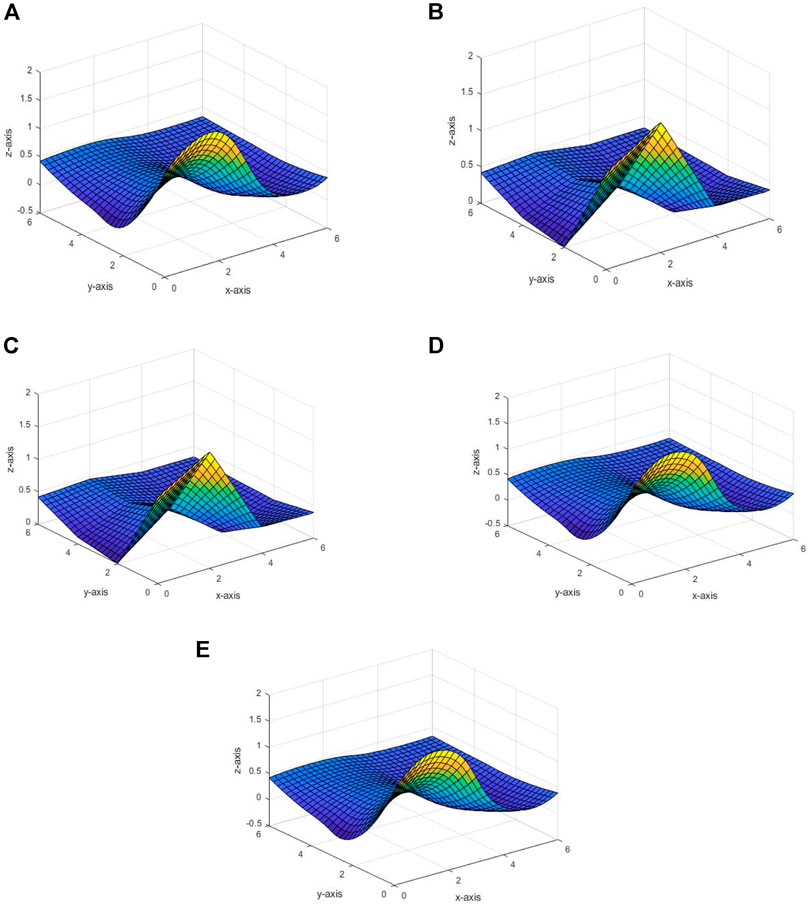
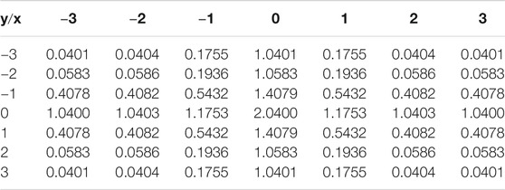
Figure 2 shows the interpolating surface by using the proposed scheme for data listed in Table 2.

Figure 2A shows the interpolating surface with ${\alpha }_{i,j}={\beta }_{i,j}=1, {\widehat{\alpha }}_{i,j}={\widehat{\beta }}_{i,j}=1$, and ${\gamma }_{i,j}={\widehat{\gamma }}_{i,j}=2.$ Meanwhile, Figure 2B shows the surface with ${\alpha }_{i,j}={\beta }_{i,j}=1, {\widehat{\alpha }}_{i,j}={\widehat{\beta }}_{i,j}=1$, and ${\gamma }_{i,j}={\widehat{\gamma }}_{i,j}=50.$ Clearly, the surfaces are bilinear or flat. A similar effect can be seen in Figure 2C, i.e., when ${\alpha }_{i,j}={\beta }_{i,j}=0.01, {\widehat{\alpha }}_{i,j}={\widehat{\beta }}_{i,j}=0.01$, and ${\gamma }_{i,j}={\widehat{\gamma }}_{i,j}=1.$Meanwhile, Figure 2D shows the behavior of the interpolating surface when ${\alpha }_{i,j}, {\beta }_{i,j}$, ${\widehat{\alpha }}_{i,j}, \text{and} {\widehat{\beta }}_{i,j}$ become a larger number, i.e., equal to 50. Finally, Figure 2E shows the surface when${\gamma }_{i,j} \text{and} {\widehat{\gamma }}_{i,j}$ become a smaller number, i.e., equal to 0.005.

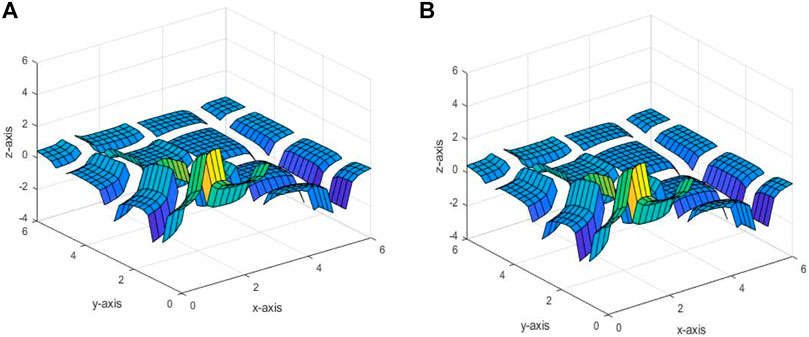
Furthermore, the parameters cannot be negative because the interpolating surface will become a rational surface, i.e., having poles on the surface. This will result in the discontinuities of the surface. This fact can be seen in Figure 3. Thus, the parameters are restricted to having positive values only. This is in line with the existing works such as Karim et al. [36], Abbas et al. [50, 51], Hussain and Ali [37], Hussain and Hussain [40], Tian et al. [41], and Sarfraz et al. [9].

Finally, as the parameters ${\alpha }_{i,j}, {\beta }_{i,j}$, ${\widehat{\alpha }}_{i,j}, \text{and} {\widehat{\beta }}_{i,j}$ are increased and ${\gamma }_{i,j}\text{ and} {\widehat{\gamma }}_{i,j}$ are fixed, we found that the rational interpolant is stable, i.e., the produced surfaces are almost identical to each other. Meanwhile, as the parameters ${\gamma }_{i,j}\text{ and} {\widehat{\gamma }}_{i,j}$ keep increasing while parameters ${\alpha }_{i,j}, {\beta }_{i,j}$, ${\widehat{\alpha }}_{i,j}, \text{and} {\widehat{\beta }}_{i,j}\text{are} \text{fixed},$we also found that the rational interpolant is stable. These results are shown in Figure 4.

FIGURE 2

FIGURE 2. Local control of surface interpolation.

TABLE 2

TABLE 2. Data from function $F_1\left(x,y\right)$.

FIGURE 3

FIGURE 3. Poles on the surface. (A)${\alpha }_{i,j}={\beta }_{i,j}= {\widehat{\alpha }}_{i,j}={\widehat{\beta }}_{i,j}=-1.$(B)${\gamma }_{i,j}={\widehat{\gamma }}_{i,j}=-2.$

FIGURE 4

FIGURE 4. Stability of the rational quartic interpolant. (A)${\alpha }_{i,j}={\beta }_{i,j}= {\widehat{\alpha }}_{i,j}={\widehat{\beta }}_{i,j}=100.$(B)${\alpha }_{i,j}={\beta }_{i,j}= {\widehat{\alpha }}_{i,j}={\widehat{\beta }}_{i,j}=1000.$(C)${\gamma }_{i,j}={\widehat{\gamma }}_{i,j}=\mathrm{0.005.}$(D)${\gamma }_{i,j}={\widehat{\gamma }}_{i,j}=\mathrm{0.0005.}$

Local Quadratic Reproducing

The proposed partially blended rational bi-quartic spline defined in Eq. 17 is local quadratic reproducing. To prove this property, we use numerical simulations by using the following quadratic test function:

$G\left(x,y\right)=x^2+y^2, -3\le x,y\le 3.$

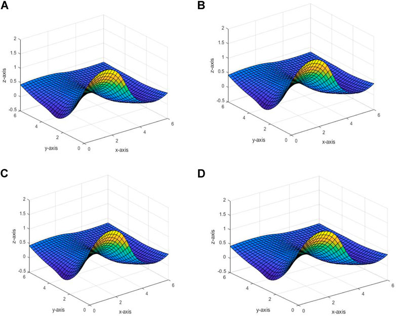
Figure 5A shows the true function. Meanwhile, Figures 5B–G show the interpolating surfaces with various parameters and their values. We can see that all figures are almost identical to each other. Table 3 shows the values of RMSE, R², and maximum absolute error for each figure. Based on Table 3, we found that as ${\gamma }_{i,j}\to 0$or ${\alpha }_{i,j},{\beta }_{i,j}\to \infty$, the proposed rational bi-quartic spline is local quadratic reproducing. This property is important since we can use our scheme to reconstruct any conic sections. Meanwhile, the works by Karim et al. [36] and Abbas et al. [50] are not local quadratic reproducing.

FIGURE 5

FIGURE 5. Local quadratic polynomial reproducing. (A) True function. (B)${\alpha }_{i,j}={\beta }_{i,j}=1, {\widehat{\alpha }}_{i,j}={\widehat{\beta }}_{i,j}=1$, and ${\gamma }_{i,j}={\widehat{\gamma }}_{i,j}=1.$(C)${\alpha }_{i,j}={\beta }_{i,j}={\widehat{\alpha }}_{i,j}={\widehat{\beta }}_{i,j}=1,{\gamma }_{i,j}={\widehat{\gamma }}_{i,j}=0.02$. (D)${\alpha }_{i,j}={\beta }_{i,j}={\widehat{\alpha }}_{i,j}={\widehat{\beta }}_{i,j}=1,{\gamma }_{i,j}={\widehat{\gamma }}_{i,j}=\mathrm{0.002.}$(E)${\beta }_{i,j}={\widehat{\alpha }}_{i,j}={\widehat{\beta }}_{i,j}=10,{\gamma }_{i,j}={\widehat{\gamma }}_{i,j}=1.$(F)${\alpha }_{i,j}={\beta }_{i,j}={\widehat{\alpha }}_{i,j}={\widehat{\beta }}_{i,j}=100,{\gamma }_{i,j}={\widehat{\gamma }}_{i,j}=1.$(G)${\alpha }_{i,j}={\beta }_{i,j}=1000,{\widehat{\alpha }}_{i,j}={\widehat{\beta }}_{i,j}=1000,\text{ and }{\gamma }_{i,j}={\widehat{\gamma }}_{i,j}=1.$

TABLE 3

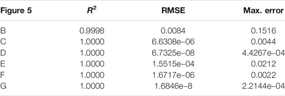
TABLE 3. Error estimation for the interpolating surface in Figure 5.

Positivity-Preserving Interpolation

The rational bi-quartic spline defined in Eq. 17 is not positivity-preserving for positive datasets. As seen in Figure 2A, the partially blended rational bi-quartic spline is not positivity-preserving interpolation. We can obtain a positive surface by manipulating all free parameters. However, this approach is not practical and really time-consuming. Therefore, we want to find an automatic method to calculate the parameter values that will produce a positive rational interpolant. To do this, we derive the sufficient condition for the positivity of the rational quartic splines on all four boundary curve networks (see Figure 1). On each boundary, there will be two free parameters. This results in eight free parameters for shape modification. The derivation of the sufficient condition is described as follows.

Let $\left(x_i,y_{i,}{F}_{i,j}\right)$ be strictly positive data (to avoid dividing by zero at later stages) defined over a rectangular grid $\left[x_i,x_{i+1}\right]\times \left[y_j,y_{j+1}\right],i=\mathrm{0,1},\mathrm{...},n-1;j=\mathrm{0,1},\mathrm{...},m-1$, such that

$F_{i,j}>0, \forall i,j.$

The partially blended rational bi-quartic spline in Eq. 17 is positive if all boundary curves defined in Eqs. 18–21 are positive, i.e., $S\left(x,y_j\right)>0, S\left(x,y_{j+1}\right)>0, S\left(x_i,y\right)>0$, and $S\left(x_{i+1},y\right)>0,$respectively. The following theorem summarizes the construction of positivity-preserving interpolation using the proposed rational bi-quartic spline.

Theorem 4. Given strictly positive surface data $F_{i,j}>0, \forall i,j,$the piecewise partially blended rational bi-quartic function $S\left(x,y\right)$ in Eq. 17 defined over the rectangular mesh $\left[x_i,x_{i+1}\right]\times \left[y_j,y_{j+1}\right],i=\mathrm{0,1},\mathrm{...},n-1;j=\mathrm{0,1},\mathrm{...},m-1$, preserves the positivity of the data if the parameters satisfy the following sufficient conditions:

$\begin{array}{l}{\alpha }_{i,j}>0,{\alpha }_{i,j+1}>0,{\beta }_{i,j}>0,{\beta }_{i,j+1}>0,{\widehat{\alpha }}_{i,j}>0,{\widehat{\alpha }}_{i+1,j}>0,{\widehat{\beta }}_{i,j}>0,{\widehat{\beta }}_{i+1,j}>0\\ {\gamma }_{i,j}>\mathrm{Max}\left\{0,-{\alpha }_{i,j}\left(h_i{F}_{i,j}^x+2F_{i,j}\right)/F_{i,j},{\beta }_{i,j}\left(h_i{F}_{i+1,j}^x-2F_{i+1,j}\right)/F_{i+1,j}\right\}\\ {\gamma }_{i,j+1}>\mathrm{Max}\left\{0,-{\alpha }_{i,j+1}\left(h_i{F}_{i,j+1}^x+2F_{i,j+1}\right)/F_{i,j+1},{\beta }_{i,j+1}\left(h_i{F}_{i+1,j+1}^x-2F_{i+1,j+1}\right)/F_{i+1,j+1}\right\}\\ {\stackrel{⌢}{\gamma }}_{i,j}>\mathrm{Max}\left\{0,-{\widehat{\alpha }}_{i,j}\left({\widehat{h}}_i{F}_{i,j}^y+2F_{i,j}\right)/F_{i,j},{\widehat{\beta }}_{i,j}\left({\widehat{h}}_j{F}_{i,j+1}^x-2F_{i,j+1}\right)/F_{i,j+1}\right\}\\ {\stackrel{⌢}{\gamma }}_{i+1,j}>\mathrm{Max}\left\{0,-{\widehat{\alpha }}_{i+1,j}\left({\widehat{h}}_i{F}_{i+1,j}^y+2F_{i+1,j}\right)/F_{i+1,j},{\widehat{\beta }}_{i+1,j}\left({\widehat{h}}_j{F}_{i+1,j+1}^y-2F_{i+1,j+1}\right)/F_{i+1,j+1}\right\}\end{array}\}.(27)$

Proof.To prove the theorem, we adopted the idea from Karim et al. [22]. As conjectured by Casciola and Romani [16], the surface is shape-preserving if all four curve networks are shape-preserving. This can be summarized as that the rational bi-quartic surface $S\left(x,y\right)$is positive if and only if all four curves are positive.From Equations (18)–(21), $S\left(x,y_j\right)>0,$ if $A_i>0, i=\mathrm{0,1,2,3.}$${\alpha }_{i,j}>0,{\beta }_{i,j}>0,{\gamma }_{i,j}>0,$$A_0>0, A_2>0, \text{and}{A}_4>0.$Therefore, $S\left(x,y_j\right)>0,$ if and only if $A_1>0$ and $A_3>0.$ Both conditions can be simplified as follows:

${\gamma }_{i,j}>-{\alpha }_{i,j}\left(h_i{F}_{i,j}^x+2F_{i,j}\right)/F_{i,j},(28)$

${\gamma }_{i,j}>{\beta }_{i,j}\left(h_i{F}_{i+1,j}^x-2F_{i+1,j}\right)/F_{i+1,j}.(29)$

Combining conditions in Eqs. 28, 29 results in the following sufficient conditions for the positivity of $S\left(x,y_j\right)$ in inequality form:

${\gamma }_{i,j}>Max\left\{0,-{\alpha }_{i,j}\left(h_i{F}_{i,j}^x+2F_{i,j}\right)/F_{i,j},{\beta }_{i,j}\left(h_i{F}_{i+1,j}^x-2F_{i+1,j}\right)/F_{i+1,j}\right\}.(30)$

Likewise, the remaining three boundary curves $S\left(x,y_{j+1}\right), S\left(x_i,y\right)$, and $S\left(x_{i+1},y\right)$ are positive if the following sufficient conditions are satisfied.$S\left(x,y_{j+1}\right)>0,$ if and only if $B_1>0$ and $B>0:$

${\gamma }_{i,j+1}>-{\alpha }_{i,j+1}\left(h_i{F}_{i,j+1}^x+2F_{i,j+1}\right)/F_{i,j+1},(31)$

${\gamma }_{i,j+1}>{\beta }_{i,j+1}\left(h_i{F}_{i+1,j+1}^x-2F_{i+1,j+1}\right)/F_{i+1,j+1}.(32)$

$S\left(x_i,y\right),$ if and only if $C_1>0$ and $C_3>0$:

${\widehat{\gamma }}_{i,j}>-{\widehat{\alpha }}_{i,j}\left({\widehat{h}}_j{F}_{i,j}^y+2F_{i,j}\right)/F_{i,j},(33)$

${\widehat{\gamma }}_{i,j}>{\widehat{\beta }}_{i,j}\left({\widehat{h}}_j{F}_{i,j+1}^y-2F_{i,j+1}\right)/F_{i,j+1}.(34)$

$S\left(x_{i+1},y\right),$ if and only if $D_1>0$ and $D_3>0$:

${\widehat{\gamma }}_{i+1,j}>-{\widehat{\alpha }}_{i+1,j}\left({\widehat{h}}_j{F}_{i+1,j}^y+2F_{i+1,j}\right)/F_{i+1,j},(35)$

${\widehat{\gamma }}_{i+1,j}>{\widehat{\beta }}_{i+1,j}\left({\widehat{h}}_j{F}_{i+1,j+1}^y-2F_{i+1,j+1}\right)/F_{i+1,j+1}.(36)$

Combining the inequality conditions stated in Eqs. 31–36 leads us to the following conditions:

$\begin{array}{c}{\gamma }_{i,j+1}>Max\left\{0,-{\alpha }_{i,j+1}\left(h_i{F}_{i,j+1}^x+2F_{i,j+1}\right)/F_{i,j+1},{\beta }_{i,j+1}\left(h_i{F}_{i+1,j+1}^x-2F_{i+1,j+1}\right)/F_{i+1,j+1}\right\} ,{\widehat{\gamma }}_{i,j}>Max\left\{0,-{\widehat{\alpha }}_{i,j}\left({\widehat{h}}_j{F}_{i,j}^y+2F_{i,j}\right)/F_{i,j},{\widehat{\beta }}_{i,j}\left({\widehat{h}}_j{F}_{i,j+1}^y-2F_{i,j+1}\right)/F_{i,j+1}\right\} ,\\ {\widehat{\gamma }}_{i+1,j}>Max\left\{0,-{\widehat{\alpha }}_{i+1,j}\left({\widehat{h}}_j{F}_{i+1,j}^y+2F_{i+1,j}\right)/F_{i+1,j},{\widehat{\beta }}_{i+1,j}\left({\widehat{h}}_j{F}_{i+1,j+1}^y-2F_{i+1,j+1}\right)/F_{i+1,j+1}\right\}.\end{array}(37)$

Then from Eqs. 30, 37, the sufficient conditions for the positivity of all the four curve networks $S\left(x,y_j\right), S\left(x,y_{j+1}\right), S\left(x_i,y\right)$, and $S\left(x_{i+1},y\right)$ are obtained. This completes the proof.The sufficient conditions in Eq. 27 can be rewritten as

$\begin{array}{l}{\alpha }_{i,j}>0,{\alpha }_{i,j+1}>0,{\beta }_{i,j}>0,{\beta }_{i,j+1}>0,{\stackrel{⌢}{\alpha }}_{i,j}>0,{\stackrel{⌢}{\alpha }}_{i+1,j}>0,{\stackrel{⌢}{\beta }}_{i,j}>0,{\stackrel{⌢}{\beta }}_{i+1,j}>0\\ {\gamma }_{i,j}>\mathrm{Max}\left\{0,-{\alpha }_{i,j}\left(h_i{F}_{i,j}^x+2F_{i,j}\right)/F_{i,j},{\beta }_{i,j}\left(h_i{F}_{i+1,j}^x-2F_{i+1,j}\right)/F_{i+1,j}\right\}\\ {\gamma }_{i,j+1}>\mathrm{Max}\left\{0,-{\alpha }_{i,j+1}\left(h_i{F}_{i,j+1}^x+2F_{i,j+1}\right)/F_{i,j+1},{\beta }_{i,j+1}\left(h_i{F}_{i+1,j+1}^x-2F_{i+1,j+1}\right)/F_{i+1,j+1}\right\}\\ {\stackrel{⌢}{\gamma }}_{i,j}>\mathrm{Max}\left\{0,-{\stackrel{⌢}{\alpha }}_{i,j}\left({\stackrel{⌢}{h}}_i{F}_{i,j}^y+2F_{i,j}\right)/F_{i,j},{\stackrel{⌢}{\beta }}_{i,j}\left({\stackrel{⌢}{h}}_j{F}_{i,j+1}^x-2F_{i,j+1}\right)/F_{i,j+1}\right\}\\ {\stackrel{⌢}{\gamma }}_{i+1,j}>\mathrm{Max}\left\{0,-{\stackrel{⌢}{\alpha }}_{i+1,j}\left({\stackrel{⌢}{h}}_i{F}_{i+1,j}^y+2F_{i+1,j}\right)/F_{i+1,j},{\stackrel{⌢}{\beta }}_{i+1,j}\left({\stackrel{⌢}{h}}_j{F}_{i+1,j+1}^y-2F_{i+1,j+1}\right)/F_{i+1,j+1}\right\}\end{array}\},(38)$

where the parameters

$k_{i,j}>0, l_{i,j}>0, m_{i,j}>0, n_{i,j}>0.$

Theorem 5. The positive partially blended rational bi-quartic spline $S\left(x,y\right)$ constructed by using shape parameters calculated using Eq. 38 is a $C^1-$continuous degree-nine piecewise rational surface with positivity-preserving properties with respect to the positive datasets.

Proof. This is a consequence from Theorem 3.The following algorithm can be used to implement the proposed positivity-preserving interpolation.

Algorithm 1

Input: Strictly positive data points$\left(x_i,y_j,F_{i,j}\right)$, $i=\mathrm{0,1},\mathrm{...},n; j=\mathrm{0,1},\mathrm{...},m.$

Output: Positive interpolating surfaces and RMSE and R² values.

Step 1: Calculate the first partial derivative values $F_{i,j}^x,F_{i,j}^y,F_{i,j}^{xy}$by using numerical techniques, i.e., AMM.

Step 2: Choose suitable positive values for free parameters${\alpha }_{i,j}, {\beta }_{i,j}, {\alpha }_{i,j+1}, {\beta }_{i,j+1}, {\widehat{\alpha }}_{i,j}, {\widehat{\alpha }}_{i+1,j}, {\widehat{\beta }}_{i,j}, {\widehat{\beta }}_{i+1,j}$, and $k_{i,j}, l_{i,j}, m_{i,j}, n_{i,j}$ and compute the values of parameters ${\gamma }_{i,j}, {\gamma }_{i,j+1}, {\widehat{\gamma }}_{i,j}, {\widehat{\gamma }}_{i+1,j}$by using Theorem 4.

Step 3: Construct the positive surfaces by substituting all the required parameters into the partially blended rational bi-quartic spline function in Eq. 17.

Repeat Steps 2 and 3 to generate a different positive surface through different positive datasets.

Results and Discussion

We test the proposed scheme by using two positive datasets. Example 2 uses the same data as in Example 1. All computational, simulation, and graphical results are obtained by using MATLAB Version 2019a installed on Windows 10, AMD Ryzen 3 2200G with Radeon Vega Graphics 3.50 GHz. As validation, we calculate RMSE and R² values and compare the results with those of Karim et al. [36] and Abbas et al. [50].

Example 2. Positive data from the following function are truncated to five decimal places [50]:

$F_1\left(x,y\right)=e^{-\left(x^2+y^2\right)/15}\left(\sin \left(x\right)+\cos \left(y\right)\right)+0.33, 0\le x,y\le 6.(39)$

Figure 6A shows the default bi-quartic Hermite spline for the positive data given in Table 4. Figures 6B,C show the xz-view and yz-view for Figure 6A, respectively. Figure 6D shows positivity-preserving by using the proposed rational bi-quartic spline with ${\alpha }_{i,j}={\beta }_{i,j}=1, {\widehat{\alpha }}_{i,j}={\widehat{\beta }}_{i,j}=1$. Meanwhile, Figures 6E,F show the xz-view and yz-view for Figure 6D, respectively. Figure 6G shows the other view for Figure 6D. Clearly, the interpolating surfaces are positive on entire given intervals. Meanwhile, Figures 6H,I show the positive interpolating surfaces using Karim et al. [36] and Abbas et al. [50] schemes.

FIGURE 6

FIGURE 6. Interpolating surface for Example 2. (A) Default surface. (B) xz-view for (A). (C) yz-view for (A). (D) The proposed scheme. (E) xz-view for (D). (F) yz-view for (D). (G) Other view for (D). (H) Karim et al. [36]. (I) Abbas et al. [1].

TABLE 4

TABLE 4. Positive surface data from function $F_1\left(x,y\right)$.

Example 3. Positive data from the following function are truncated to four decimal places [51]:

$F_3\left(x,y\right)=e^{-x^2}+e^{-2y^2}+0.04, -3\le x,y\le 3.(41)$

Figure 7A shows the default bi-quartic Hermite spline for the positive data given in Table 5. Figures 7B,C show the xz-view and yz-view for Figure 7A, respectively. Figure 7D shows positivity-preserving by using the proposed rational bi-quartic spline with ${\alpha }_{i,j}={\beta }_{i,j}=1, {\widehat{\alpha }}_{i,j}={\widehat{\beta }}_{i,j}=1$. The parameters ${\gamma }_{i,j} \text{and} {\widehat{\gamma }}_{i,j}$ are obtained by applying Theorem 4, i.e., Eq. 27. Meanwhile, Figures 8E,F show the xz-view and yz-view for Figure 8D, respectively. Figure 7G shows the other view for Figure 7A. Meanwhile, Figure 7H shows the other view for the surface in Figure 8D. We found that the interpolating surfaces are positive everywhere. Figures 7I,J show the interpolating surfaces using Karim et al. [36] and Abbas et al. [50] schemes.

FIGURE 7

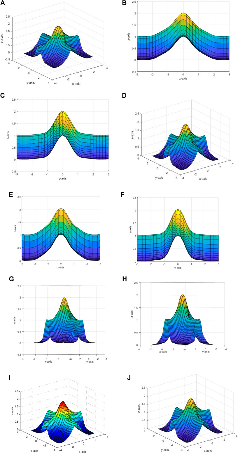
FIGURE 7. Interpolating surface using the proposed scheme for Example 3. Interpolating surfaces for data in Table 5. (A) Default surface. (B) xz-view for (A). (C) yz-view for (A). (D) The proposed scheme. (E) xz-view for (D). (F) yz-view for (D). (G) Other view for (A). (H) Other view for (D). (I) Karim et al. [36]. (J) Abbas et al. [1].

TABLE 5

TABLE 5. Positive surface data from function $F_3\left(x,y\right)$.

FIGURE 8

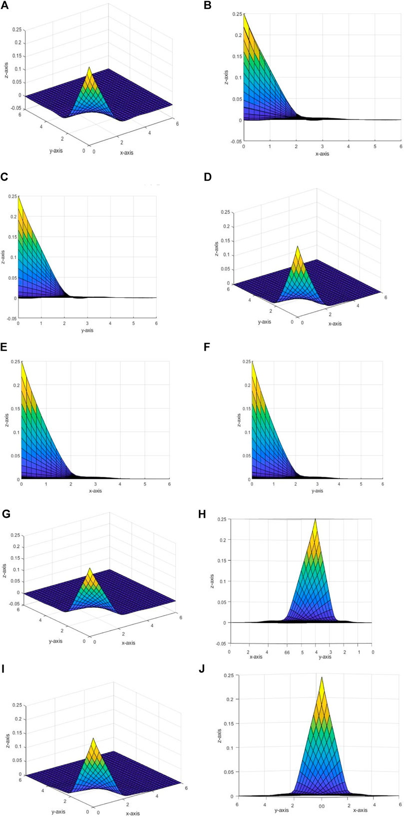
FIGURE 8. Various interpolating surfaces. (A) Default surface. (B) xz-view for (A). (C) yz-view for (A). (D) Positivity-preserving surface. (E) xz-view for (D). (F) yz-view for (D). (G) Non-positivity-preserving surface. (H) Other view for (G). (I) Positivity-preserving surface. (J) Other view for (I).

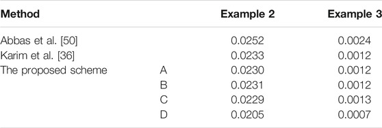
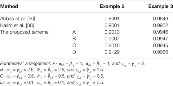
We compare the performance between the proposed partially blended rational bi-quartic spline interpolation and the works of Abbas et al. [50] and Karim et al. [36] by calculating the root mean square error (RMSE) and coefficient of determination (R²). Tables 6, 7 summarize the main results. It can clearly be seen that the proposed rational bi-quartic spline interpolation is on par with the works of Abbas et al. [50] and Karim et al. [36]. Based on R², for both examples, the proposed scheme is the best. Furthermore, according to Renka and Brown [53] criteria, the proposed scheme is excellent since the R² value is in between 0.91 and 0.997. Meanwhile, based on the RMSE value, we found that the proposed scheme is the best when the parameters are ${\alpha }_{i,j}={\beta }_{i,j}=0.1 \text{and}{\widehat{\alpha }}_{i,j}={\widehat{\beta }}_{i,j}=\mathrm{0.1.}$ From all numerical simulations, we found that the proposed scheme requires less computation times (in seconds) compared with Abbas et al. [50] and Karim et al. [36] schemes. The speedup is around 10% faster than the other schemes. Furthermore, based on graphical results, all schemes are looking competent to each other. Most probably, the proposed scheme is the best for both examples. Based on this, we conclude that the rank from the best scheme to the lowest is as follows:

TABLE 6

TABLE 6. Root mean square error (RMSE) values.

TABLE 7

TABLE 7. Coefficient of determination (R²) values.

The Proposed Scheme > Karim et al. [36] > Abbas et al. [50]

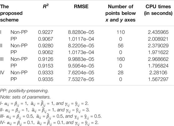
Our final example shows that the proposed rational bi-quartic spline for positivity-preserving has the capability to reduce the CPU times (in seconds) to construct the interpolating surface compared with interpolation without positivity-preserving. Table 8 shows the positive data from the following function:

$F_3\left(x,y\right)=\frac{0.25}{\left({\left(x^2+y^2\right)}^2+1\right)}, 0\le x,y\le 6.(42)$

Figure 8 shows the examples of various interpolating surfaces for data given in Table 8. Figure 8A shows the interpolating surface when the free parameters are ${\alpha }_{i,j}={\beta }_{i,j}=1, {\widehat{\alpha }}_{i,j}={\widehat{\beta }}_{i,j}=1$, and ${\gamma }_{i,j}={\widehat{\gamma }}_{i,j}=2.$Figures 8B,C show the xz-view and yz-view for Figure 8A. Clearly, the surfaces are not positive everywhere. Figure 8D shows the positive interpolating surface after applying Theorem 4. The free parameters are ${\alpha }_{i,j}={\beta }_{i,j}=1, \text{and} {\widehat{\alpha }}_{i,j}={\widehat{\beta }}_{i,j}=1$. Meanwhile, ${\gamma }_{i,j}\text{ and }{\widehat{\gamma }}_{i,j}$ are obtained through Eq. 27. Figures 8E,F show the xz-view and yz-view for Figure 8D. From both graphs, the surfaces are positive and lie above both x and y axes. Figure 8G shows another interpolating surface with parameters ${\alpha }_{i,j}={\beta }_{i,j}=0.1, {\widehat{\alpha }}_{i,j}={\widehat{\beta }}_{i,j}=0.1$. However, the surface is not positive as seen in Figure 8H. Finally, Figure 8I shows the interpolating surface using the proposed scheme. From Figure 8J, it is seen that the interpolating surface shown in Figure 8I is positive everywhere. Therefore, Theorem 4 is confirmed to produce a positive interpolating surface on entire given intervals. This is in contrast with what was claimed by Qin et al. [38]. Therefore, the proposed scheme indeed has reduced the number of mathematical derivations needed to produce a positive rational interpolant. This is very significant in numerical analysis aspects. We only require lesser computation time compared with the work of Qin et al. [38]. CPU times (in seconds) are measured by using MATLAB tic and toc commands.

TABLE 8

TABLE 8. Positive surface data from function $F_3\left(x,y\right)$.

As seen in Table 9, by applying the positivity-preserving interpolation scheme to the given data, the CPU times (in seconds) needed to construct the interpolating surface are reduced. This is true for all set of parameters. We also noticed that the proposed sufficient condition for the positivity of the rational quartic interpolant is guaranteed to produce a positive interpolating surface everywhere, i.e., on entire given intervals. However, we also found that, by applying positivity-preserving interpolation, R² values will be reduced, while at the same time, the RMSE value will be increased. However, the values are not much different.

TABLE 9

TABLE 9. Error estimation.

Final Remark: Qin et al. [38] have proposed a new approach to derive the sufficient condition for the positivity of the partially blended rational spline. They claimed that their condition is guaranteed to produce a positive interpolating surface everywhere. However, their method is mathematically more complicated to apply since it will increase the unnecessary computation time to produce the positive surface. If we apply the Qin et al. [38] method, the sufficient condition for the positivity of the rational quartic spline will take the following form:

$S\left(x,y_j\right)-\frac{1}{2}{a}_0\left(\theta \right)F_{i,j}-\frac{1}{2}{a}_1\left(\theta \right)F_{i+1,j}>0,(43)$

$S\left(x,y_{j+1}\right)-\frac{1}{2}{a}_0\left(\theta \right)F_{i,j+1}-\frac{1}{2}{a}_1\left(\theta \right)F_{i+1,j+1}>0,(44)$

$S\left(x_i,y\right)-\frac{1}{2}{a}_0\left(\theta \right)F_{i,j}-\frac{1}{2}{a}_1\left(\theta \right)F_{i,j+1}>0,(45)$

$S\left(x_{i+1},y\right)-\frac{1}{2}{a}_0\left(\theta \right)F_{i,j}-\frac{1}{2}{a}_1\left(\theta \right)F_{i+1,j+1}>0.(46)$

It is very complicated to solve Eq. 43 until Eq. 46. This is because we need to simplify all equations to form a new rational function, i.e., quintic numerator and quadratic denominator. Compared with our derivation for the positivity of the rational quartic spline which is direct and easy as shown in Eq. 28 until Eq. 36. Furthermore, based on all numerical and graphical results presented in this study, we found that the sufficient condition on all four curve networks is sufficient to produce positive interpolating surfaces on the entire given domain and not just on the four boundary curves only. This fact can be seen clearly in the final example. When we applied the proposed scheme, we found that, without positivity-preserving interpolation, the z values are negative. Meanwhile, after we apply the sufficient condition stated in Theorem 4, we obtain the interpolating surface as positive everywhere as seen in Figures 6–8 as well as in Table 9. Therefore, we encouraged the user to use our proposed rational bi-quartic spline for positivity-preserving interpolation with the following merits:

1) It will guarantee to produce a positive interpolating surface on entire given intervals and not just on the four boundary curve networks as claimed by Qin et al. [38]. From all numerical examples, we found that, after the positivity conditions are applied, all points on the surface are positive.

2) It can reproduce an exactly quadratic polynomial unlike Abbas et al. [50], Karim et al. [36], and Qin et al. [38].

3) Overall, based on R² and RMSE values, the proposed scheme is the best compared with some existing schemes.

Conclusion

In this study, a new partially blended rational bi-quartic spline interpolation with C¹ continuity is constructed for positivity-preserving application. The sufficient condition for the positivity of the rational quartic spline is derived on four boundary curves defined on rectangular meshes. This condition results in eight free parameters for shape modification. The proposed scheme is tested for many positive surface datasets. Based on numerical analysis and graphical comparison, the proposed scheme is the best, i.e., higher R² and smaller RMSE. We also found that the proposed scheme has the capability to reduce the CPU times (in seconds) when we want to construct a positive interpolating surface. Furthermore, the proposed positivity-preserving interpolation scheme is guaranteed to deliver a positive surface on the entire given interval. The derivation for the positivity sufficient condition in this study is easier than that in the study of Qin et al. [38]. By using our proposed scheme, we have reduced the required numbers of mathematical derivations, and our scheme is easy to use. On top of that, the proposed scheme is local quadratic polynomial reproducing. This is significant when the user wants to reconstruct any quadric surfaces. Future studies will be focusing on the construction of general shape-preserving for scattered data arranged on triangular meshes as well as its applications in image processing and image denoising such as in the studies of Karim and Saaban [55], Karim et al. [56], Walther and Schmidt [57], and Zulkifli et al. [58].

Data Availability Statement

The original contributions presented in the study are included in the article/supplementary material, and further inquiries can be directed to the corresponding author.

Author Contributions

SA, AS, and VN curated the data, involved in formal analysis, obtained the resources, and wrote the original draft. SA and VN performed the methodology. SA acquired the funding and investigated the data. VN involved in project administration. SA and AS ran the software, validated and visualized the results, and reviewed and edited the paper.

Funding

The authors would like to acknowledge Universiti Teknologi PETRONAS (UTP) and Ministry of Education (MOE), Malaysia, for the financial support received in the form of a research grant: FRGS/1/2018/STG06/UTP/03/1/015MA0-020 and YUTP: 015LC0-315 (Uncertainty estimation based on quasi-Newton methods for Full Waveform Inversion (FWI)).

Conflict of Interest

The authors declare that the research was conducted in the absence of any commercial or financial relationships that could be construed as a potential conflict of interest.

Publisher’s Note

All claims expressed in this article are solely those of the authors and do not necessarily represent those of their affiliated organizations, or those of the publisher, the editors and the reviewers. Any product that may be evaluated in this article, or claim that may be made by its manufacturer, is not guaranteed or endorsed by the publisher.

References

1. Duan Q, Djidjeli K, Price WG, Twizell EH. Constrained Control and Approximation Properties of a Rational Interpolating Curve. Inf Sci (2003) 152:181–94. doi:10.1016/s0020-0255(02)00409-7

CrossRef Full Text | Google Scholar

2. Duan Q, Wang L, Twizell EH. A New Bivariate Rational Interpolation Based on Function Values. Inf Sci (2004) 166:181–91. doi:10.1016/j.ins.2003.12.001

CrossRef Full Text | Google Scholar

3. Duan Q, Zhang H, Zhang Y, Twizell EH. Bounded Property and Point Control of a Bivariate Rational Interpolating Surface. Comput Math Appl (2006) 52:975–84. doi:10.1016/j.camwa.2006.04.021

CrossRef Full Text | Google Scholar

4. Duan Q, Bao F, Zhang Y. Shape Control of a Bivariate Interpolating Spline Surface. Int J Comp Math (2008) 85(No. 5):813–25. doi:10.1080/00207160701463245

CrossRef Full Text | Google Scholar

5. Farin GE. Curves and Surfaces for CAGD: A Practical Guide. 5th ed. San Francisco, CA: Morgan Kaufmann Publishers (2002).

6. Brodlie KW, Butt S. Preserving Convexity Using Piecewise Cubic Interpolation. Comput Graphics (1991) 15(1):15–23. doi:10.1016/0097-8493(91)90026-e

CrossRef Full Text | Google Scholar

7. Brodlie K, Mashwama P, Butt S. Visualization of Surface Data to Preserve Positivity and Other Simple Constraints. Comput Graphics (1995) 19(4):585–94. doi:10.1016/0097-8493(95)00036-c

CrossRef Full Text | Google Scholar

8. Butt S, Brodlie KW. Preserving Positivity Using Piecewise Cubic Interpolation. Comput Graphics (1993) 17(1):55–64. doi:10.1016/0097-8493(93)90051-a

CrossRef Full Text | Google Scholar

9. Sarfraz M, Hussain MZ, Nisar A. Positive Data Modeling Using Spline Function. Appl Math Comput (2010) 216:2036–49. doi:10.1016/j.amc.2010.03.034

CrossRef Full Text | Google Scholar

10. Beliakov G. Monotonicity Preserving Approximation of Multivariate Scattered Data. Bit Numer Math (2005) 45(4):653–77. doi:10.1007/s10543-005-0028-x

CrossRef Full Text | Google Scholar

11. Asim MR, Mustafa G, Brodlie KW. Constrained Visulaization of 2D Positive Data Using Modified Quadratic Shepard Method. MSCG POSTERS Proceedings, WSCG’2004. Plzen, Czech Republic. Curve drawing subject to positivity and more general constraints. Comput Graphics (2004) 27:469–85.

Google Scholar

12. Bao F, Sun Q, Duan Q. Point Control of the Interpolating Curve with a Rational Cubic Spline. J Vis Commun Image Representation (2009) 20:275–80. doi:10.1016/j.jvcir.2009.03.003

CrossRef Full Text | Google Scholar

13. Wu J, Zhang X, Peng L. Positive Approximation and Interpolation Using Compactly Supported Radial Basis Functions. Math Probl Eng (2010) 2010. doi:10.1155/2010/964528

CrossRef Full Text | Google Scholar

14. Wu J, Lai Y, Zhang X. Radial Basis Functions for Shape Preserving Planar Interpolating Curves. J Inf Comput Sci (2010) 7(7):1453–8.

Google Scholar

15. Zhu Y. C2 Positivity-Preserving Rational Interpolation Splines in One and Two Dimensions. Appl Math Comput (2018) 316:186–204. doi:10.1016/j.amc.2017.08.026

CrossRef Full Text | Google Scholar

16. Casciola G, Romani L. Rational Interpolants with Tension Parameters, In: Lyche T, Mazure M-L, and Schumaker LL, editors Curve and Surface Design. Nashboro Press (2003). pp. 41–50.

17. Schmidt JW, Hess W. Positive Interpolation with Rational Quadratic Splines. Computing (1987) 38:261–7. doi:10.1007/bf02240100

CrossRef Full Text | Google Scholar

18. Schmidt JW, Hess W. Positivity of Cubic Polynomials on Intervals and Positive Spline Interpolation. BIT (1988) 28:340–52. doi:10.1007/bf01934097

CrossRef Full Text | Google Scholar

19. Schmidt JW. Positivity, Monotone and -convex Interpolation on Rectangular Grids. Computing (1992) 48(3-4):363–71. doi:10.1007/bf02238643

CrossRef Full Text | Google Scholar

20. Hussain MZ, Sarfraz M, Shakeel A. Shape Preserving Surfaces for the Visualization of Positive and Convex Data Using Rational Bi-quadratic Splines. Int J Compu Appl (2011) 27(10):12–20.

Google Scholar

21. Chan ES, Ong BH. Range Restricted Scattered Data Interpolation Using Convex Combination of Cubic Bézier Triangles. J Comput Appl Math (2001) 136:135–47. doi:10.1016/s0377-0427(00)00580-x

CrossRef Full Text | Google Scholar

22. Luo Z, Peng X. A C1-Rational Spline in Range Restricted Interpolation of Scattered Data. J Comput Appl Math (2006) 194(2):255–66. doi:10.1016/j.cam.2005.07.010

CrossRef Full Text | Google Scholar

23. Piah ARM, Goodman TNT, Unsworth K. Positivity-preserving Scattered Data Interpolation. Lecture Notes Comp Sci (LNCS) (2005) 3604:336–49. doi:10.1007/11537908_20

CrossRef Full Text | Google Scholar

24. Hussain MZ, Hussain M. C1 Positive Scattered Data Interpolation. Comput Math Appl (2010) 59:457–67. doi:10.1016/j.camwa.2009.06.019

Google Scholar

25. Saaban A, Majid AA, Piah ARM. Visualization of Rainfall Data Distribution Using Quintic Triangular Bezier Patches. Bull Malays Math Sci Soc (2009) 32(2):137–50.

Google Scholar

26. Hussain MZ, Hussain M, Samreen S. Visualization of Shaped Data by Rational Quartic Spline Interpolation. Int J Appl Math Stat (2008) 13(J08):34–46.

Google Scholar

27. Hussain MZ, Hussain M. Visualization of 3D Data Preserving Convexity. J Appl Math Comput (2007) 23(2):397–410. doi:10.1007/bf02831986

CrossRef Full Text | Google Scholar

28. Wang Q, Tan J. Rational Quartic Spline Involving Shape Parameters. J Inf Comput Sci (2004) 1(1):127–30.

Google Scholar

29. Harim NA, Karim AAA, Othman O, Saaban A, Ghaffar A, Nisar KS, et al. Positivity Preserving Interpolation by Using Rational Quartic Spline. AIMS Math (2020) 5(4):3762–82. doi:10.3934/math.2020244

CrossRef Full Text | Google Scholar

30. Liu X, Zhu Y, Liu S. Positivity and Monotonicity Preserving Biquartic Rational Interpolation Spline Surface. J Appl Math (2014) 2014:11 Article ID 987076. doi:10.1155/2014/987076

CrossRef Full Text | Google Scholar

31. Hussain MZ, Sarfraz M. Positivity-Preserving Interpolation of Positive Data by Rational Cubics. J Comput Appl Math (2008) 218:446–58. doi:10.1016/j.cam.2007.05.023

CrossRef Full Text | Google Scholar

32. Han X. Convexity-preserving Piecewise Rational Quartic Interpolation. SIAM J Numer Anal (2008) 46(2):920–9. doi:10.1137/060671577

CrossRef Full Text | Google Scholar

33. Han X. Shape-preserving Piecewise Rational Interpolant with Quartic Numerator and Quadratic Denominator. Appl Math Comput (2015) 251:258–74. doi:10.1016/j.amc.2014.11.067

CrossRef Full Text | Google Scholar

34. Harim AN, Karim SAA, Othman M, Saaban A, Ghaffar A, Nisar KS, et al. Positivity Preserving Interpolation by Using Rational Quartic Spline. AIMS Math (2020) 5(4):3762–82. doi:10.3934/math.2020244

Google Scholar

35. Harim A, Karim SAA, Othman M, Saaban A. High Accuracy Data Interpolation Using Rational Quartic Spline with Three Parameters. Int J Scientific Tech Res (2019) 1219–27432.

Google Scholar

36. Karim SAA, Kong VP, Saaban A. Positivity Preserving Interpolation Using Rational Bi-cubic Spline. J Appl Math (2015) 2015. doi:10.1155/2015/572768

CrossRef Full Text | Google Scholar

37. Hussain MZ, Ali JM. Positivity Preserving Piecewise Rational Cubic Interpolation. Matematika (2006) 22(2):147–53.

Google Scholar

38. Qin X, Qin L, Xu Q. C¹ Positivity-Preserving Interpolation Schemes with Local Free Parameters. IAENG Int J Comp Sci (2016) 43(2).

Google Scholar

39. Gregory JA. Shape Preserving Spline Interpolation. Computer-Aided Des (1986) 18(1):53–7. doi:10.1016/s0010-4485(86)80012-4

CrossRef Full Text | Google Scholar

40. Hussain MZ, Hussain M. Visualization of Data Subject to Positive Constraint. J Inf Comput Sci (2006) 1(3):149–60.

Google Scholar

41. Tian M, Zhang Y, Zhu J, Duan Q. Convexity-Preserving Piecewise Rational Cubic Interpolation. J Inf Comput Sci (2005) 2(4):799–803.

Google Scholar

42. Hussain MZ, Sarfraz M, Shaikh TS. Shape Preserving Rational Cubic Spline for Positive and Convex Data. Egypt Inform J (2011) 12:231–6. doi:10.1016/j.eij.2011.10.002

CrossRef Full Text | Google Scholar

43. Ashraf P, Sabir M, Ghaffar A, Nisar KS, Khan I. Shape-Preservation of the Four-Point Ternary Interpolating Non-stationary Subdivision Scheme. Front Phys (2020) 7:241. doi:10.3389/fphy.2019.00241

CrossRef Full Text | Google Scholar

44. Fiorot JC, Tabka J. Shape-Preserving C 2 Cubic Polynomial Interpolating Splines. Math Comput (1991) 57:291–8. doi:10.2307/2938674

CrossRef Full Text | Google Scholar

45. Peng X, Li Z, Sun Q. Nonnegativity Preserving Interpolation by Bivariate Rational Spline Surface. J Apllied Math (2012) 2012:Article ID 624978.

Google Scholar

46. Fritsch FN, Butland J. A Method for Constructing Local Monotone Piecewise Cubic Interpolants. SIAM J Sci Stat Comput (1984) 5:300–4. doi:10.1137/0905021

CrossRef Full Text | Google Scholar

47. Fritsch FN, Carlson RE. Monotone Piecewise Cubic Interpolation. SIAM J Numer Anal (1980) 17:238–46. doi:10.1137/0717021

CrossRef Full Text | Google Scholar

48. Wang Q, Tan J. Shape Preserving Piecewise Rational Biquartic Surface. J Inf Comput Sci (2006) 3:295–302.

Google Scholar

49. Wang Y, Tan J, Li Z, Bai T. Weighted Rational Quartic Spline Interpolation. J Inf Comput Sci (2013) 10(9):2651–8. doi:10.12733/jics20101820

CrossRef Full Text | Google Scholar

50. Abbas M, Majid AA, Ali JM. Shape Preserving Rational Bi-cubic Function for Positive Data. World Appl Sci J (2012) 18(11):1671–9. doi:10.5829/idosi.wasj.2012.18.11.3527

Google Scholar

51. Abbas M, Majid AA, Ali JM. Positivity-preserving Rational Bi-cubic Spline Interpolation for 3D Positive Data. Appl Math Comput (2014) 234:460–76. doi:10.1016/j.amc.2014.02.031

CrossRef Full Text | Google Scholar

52. Ibraheem F, Hussain M, Hussain MZ, Bhatti AA. Positive Data Visualization Using Trigonometric Polynomials. J Appl Math (2012) 2012:19 Article ID 247120. doi:10.1155/2012/247120

CrossRef Full Text | Google Scholar

53. Renka RG, Brown R. Algorithm 792: Accuracy Tests of ACM Algorithms for Interpolation of Scattered Data in the Plane. ACM Trans Math Softw (1999) 25:1. doi:10.1145/305658.305745

CrossRef Full Text | Google Scholar

54. Delbourgo R, Gregory JA. The Determination of Derivative Parameters for a Monotonic Rational Quadratic Interpolant. IMA J Numer Anal (1985) 5:397–406. doi:10.1093/imanum/5.4.397

CrossRef Full Text | Google Scholar

55. Karim SAA, Saaban A. Shape Preserving Interpolation and its Application in Image Processing. Math Problem Eng (2017) 12:7459218. doi:10.1155/2017/7459218

CrossRef Full Text | Google Scholar

56. Karim SAA, Saaban A, Skala V. Range-Restricted Surface Interpolation Using Rational Bi-cubic Spline Functions with 12 Parameters. IEEE Access (2019) 7:104992–5007. doi:10.1109/ACCESS.2019.2931454

CrossRef Full Text | Google Scholar

57. Walther MB, Schmidt JW. Range Restricted Interpolation Using Gregory’s Rational Cubic Splines. J Comput Appl Math (1999) 103:221–37.

Google Scholar

58. Zulkifli NA, Karim SAA, Shafie A, Sarfraz M, Ghaffar A, Nisar KS. Image Interpolation Using a Rational Bi-cubic Ball. Mathematics (2019) 7:1045. doi:10.3390/math7111045

CrossRef Full Text | Google Scholar