 Alicia Castro
 Tim Andreas Koslowski
- 1Radboud University Nijmegen, Nijmegen, Netherlands
- 2Julius Maximilian University of Würzburg, Würzburg, Germany
This contribution is not intended as a review but, by suggestion of the editors, as a glimpse ahead into the realm of dually weighted tensor models for quantum gravity. This class of models allows one to consider a wider class of quantum gravity models, in particular one can formulate state sum models of spacetime with an intrinsic notion of foliation. The simplest one of these models is the one proposed by Benedetti and Henson [1], which is a matrix model formulation of two-dimensional Causal Dynamical Triangulations (CDT). In this paper we apply the Functional Renormalization Group Equation (FRGE) to the Benedetti-Henson model with the purpose of investigating the possible continuum limits of this class of models. Possible continuum limits appear in this FRGE approach as fixed points of the renormalization group flow where the size of the matrix acts as the renormalization scale. Considering very small truncations, we find fixed points that are compatible with analytically known results for CDT in two dimensions. By studying the scheme dependence of our results we find that precision results require larger truncations than the ones considered in the present work. We conclude that our work suggests that the FRGE is a useful exploratory tool for dually weighted matrix models. We thus expect that the FRGE will be a useful exploratory tool for the investigation of dually weighted tensor models for CDT in higher dimensions.
1 Introduction
The construction of a unified theory that contains the two most successful branches of modern physics, i.e. General Relativity (GR) and Quantum Field Theory (QFT) in a curved spacetime, as appropriate limits has been ongoing for more than 80 years and sparked many approaches to the so-called problem of quantum gravity. A complete list of these approaches goes beyond the scope of this introduction. The approaches range from the very conservative application of QFT [2, 3] methods to theories of gravity and the asymptotic safety conjecture [4–6] over refined applications of quantization rules, such as loop quantum gravity [7], spin foams [8], group field theories [9] and tensor models [10–13] to significantly less conservative approaches like emergent gravity [14], holographic duality [15] and to searches for so-called theories of everything such as string theory [16]. Despite the significant diversity, no approach has produced a completely satisfactory answer to the problem of quantum gravity as of now. However, when comparing different approaches, one is lead to the general observation that most of them possess some built-in features that one expects from quantum gravity, but all known approaches come with intrinsic short-comings that have to be overcome before qualifying the particular approach as a candidate theory of quantum gravity. This observation suggests to combine formulations with different built-in strengths with the goal of obtaining a new approach that mixes the best of both.
The present contribution intends precisely this by combining the systematic renormalization group investigation of tensor models for quantum gravity with the success of CDT in producing phases in which the partition function is dominated by extended geometries [17]. This combination is most straightforwardly possible when CDT is formulated as a dually weighted tensor model. Before going into detail, let us take a step back and describe the big picture schematically:
Tensor models of quantum gravity are based on the principles of Euclidean lattice quantum gravity. Euclidean lattice quantum gravity is a partition function approach, where the partition function is obtained as a sum over Boltzmann factors for spacetimes that are constructed from discrete building blocks. The continuum limit of these partition functions is taken as the limit in which the size of the building blocks approaches zero, while the total volume of the spacetime is held fixed. This implies that the number of building blocks has to diverge when taking the continuum limit, thus indicating that one needs to consider the renormalization group flow of these partition functions, such that the possible continuum limits are identified as the classes of IR-relevant deformations of UV-attractors (in most cases fixed points) of the renormalization group flow. A particularly useful tool for the systematic investigation of non-perturbative renormalization group flow is the FRGE, which takes the form of a simple one-loop equation that describes an interpolation between a bare action and the quantum effective action [18]. To apply this powerful tool to Euclidean lattice gravity it is very useful to exploit the duality between the Feynman-graphs of (un)-colored1 tensor models and discrete geometries. This duality allows one to identify the Feynman amplitude of the (un)-colored tensor model with the Boltzmann factor of the associated discrete gravity partition function and hence allows a translation from the tensor model action to the discrete gravity action, which takes the form of a Regge action [19]. Thus, the duality relates the large N-limit of the tensor model with the continuum limit of the discrete gravity partition function. Hence, the investigation of continuum limits of lattice quantum gravity is readily translated into the investigation of the possible large N-limits of tensor models, which can be investigated systematically using the FRGE.
This rigorous connection between the continuum limit of Euclidean lattice quantum gravity and the large N-renormalization group flow of tensor model actions is an invaluable intrinsic feature of the tensor model approach to quantum gravity; and the systematic investigation of these continuum limits with the FRGE is particularly convenient. Unfortunately, the extended geometries that are approximated in the continuum limits that have been investigated so far possess dimension two or less [20]. In other words, so far no state sum model of discrete geometry is known to coarse grain to a model of extended spacetime geometry in more than two dimensions.
There are however numerical indications that d-dimensional CDT and its counter part Euclidean Dynamical Triangulations (EDT) do coarse grain to extended higher dimensional geometries (for 2 ≤ d ≤ 4) [21]. This can be heuristically understood as the fact that the foliation in CDT and the volume term in EDT implement additional terms in the Boltzmann factor for discrete geometry which change the universality class of the model. Moreover, there exist tensor models that implement critical of features of CDT and EDT partition functions in the literature. The novelty in these models is that they possess a nontrivial propagator, which implements a dual weighting of the Feynman graphs of these tensor models. Hence, one can use the FRGE to investigate the continuum limits of CDT and EDT by studying the renormalization group flow of tensor models with dual weights. This is the motivation for the work presented in the present contribution.
As a first step, we consider a dually weighted matrix model proposed by Benedetti and Henson whose partition function is dual to two-dimensional CDT [22]. By doing this we follow a strategy that was used when first applying the FRGE to tensor models [23], where matrix models for two-dimensional Euclidean quantum gravity were considered to introduce the setup, develop the technique and to compare with the analytic results known from constructive approaches to two-dimensional Euclidean quantum gravity, which serve as a benchmark. This allows us to test a setup (the systematic FRGE investigation to dually weighted tensor models) that is readily available in higher dimensions, in particular in 3 + 1 dimensions [22], but at the same time is understood analytically, providing benchmark results for the FRGE calculation which we can use to gauge this setup.
This contribution is organized as follows: In the following section (Preliminaries) we provide the necessary background on dually weighted tensor models, the particular model proposed by Benedetti and Henson and the foundations of the application of the FRGE to tensor models. We provide the derivation of the beta functions in β-functions. We perform a fixed point analysis and study of scheme dependence in Fixed Point Analysis and Scheme Dependence. We summarize our results in Conclusion and briefly discuss their implications for future investigations on dually weighted tensor models for quantum gravity and provide a short recipe for the calculation in the appendix.
2 Preliminaries
Random tensor models are by now an established approach to Euclidean quantum gravity [24, 25]. However, to fully appreciate the way in which dually weighted matrix models provide an approach to quantum gravity with a preferred time slicing one needs to take a step back and consider the foundations of random tensor models.
2.1 Tensor Models and Dual Weights
The random tensor model approach to quantum gravity is based on the basic observation that the Feynman graphs of so-called uncolored random tensor models possess a geometric interpretation in terms of tessellations of piece-wise linear pseudo-manifolds, as do some so-called colored tensor models. The uncolored models are defined for tensors
This symmetry implies that the action can be expanded in terms of generalized trace invariants in which the first index i1 of each tensor T must be contracted with the first index of a complex conjugated tensor
We can perform the analogous identification for the Feynman graphs generated by the rank k random tensor model through realizing that the Feynman graphs of a rank k tensor model possess a graphical representation in terms of (k+1)-colored graphs, where a new color is associated with the propagator. This provides the desired geometric interpretation of the Feynman graphs of an uncolored rank k tensor model with tessellations Δ of piecewise linear pseudo-manifolds of dimension k. It follows that the partition function of these random tensor models possesses a geometric interpretation
Where
When the gravity action SE[Δ,a] is identified with
Where the couplings N,λ possess a simple relation with the couplings in the Regge-expression of General Relativity in three dimensions SR[Δ] = κ3N3−κ1N1. Hence, κ1 = 1n(N) and
The total volume is
So far we have only considered a canonical quadratic term
2.2 Application of the FRGE to Tensor Models
One of the most convenient tools to investigate critical behavior is the functional renormalization group equation (FRGE). In the usual setting the FRGE
Describes how the effective average action
Changes when the IR suppression scale k is changed. This IR-suppression scale is introduced through a modification of the bare action by the scale dependent mass term ΔkS[ϕ] = 1/2ϕRkϕ, which is designed to give a mass of
The usual FRGE arguments outlined above relies heavily on the mass dimension and scaling with a scale k that possesses units of mass. Such a mass scale is missing in the random tensor setup, instead one wants to study the scaling of the couplings with the dimensionless tensor size N. This requires one to identify 1) the scaling of the IR-suppression term with N and 2) the scaling of the coupling constants with N. It turns out that the requirement that the RHS of the FRGE admits a 1/N-expansion imposes significant restrictions on the scaling with N, but it does not fix it completely. To obtain a completely determined scaling with N one needs to impose that the bare action possesses a geometric interpretation. Essentially, the requirements are that (1) the bare propagator and the modified propagator (after including the IR-suppression term ΔNS[T]) possess the same scaling for large index values and 2) that the interaction term possesses the scaling necessary for the geometric interpretation. These two initial conditions, together with the restrictions that result from the 1/N-expandability of the RHS of the FRGE fix the setting that is sufficient to investigate the large-N-critical behavior.
2.3 2D Causal Matrix Model
A matrix model that enforces a preferred time slicing in its Feynman-graphs was proposed by Benedetti and Henson in [1]. This model is constructed using two dynamical N × N matrices, A and B, representing the spacelike and timelike edges of a triangle, and a constant matrix C which implements the dual weighting. The partition function is
Where in the large N limit the matrix C must satisfy the condition
With
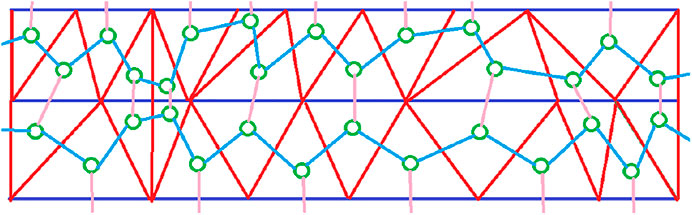
FIGURE 1. Part of a dual triangulation to a Feynman graph. The solid colors red and blue indicate the time- and space-like boundaries of dual triangles, the light colors the dual propagators in the Feynman graph and the green circles the vertices in the Feynman graph. The important fact to note is that having precisely two pink propagators in each closed loop implies that the blue lines foliate the entire Feynman graph. Notice that we drew the propagators as single lines to not clutter the picture too much; the usual depiction of the matrix model propagator would be though a double line, i.e. line one for each contacted index.
As we can see in Figure 1, this restriction implements a foliation of the discrete geometries that appear in the expansion of the partition function, thus introducing the necessary structure for the implementation of CDT in tensor models.
We proceed by integrating out matrix B since it is a gaussian integral, obtaining
This partition function together with condition (8) determines our starting point in this work.
One can understand the integration over matrix B as the gluing of triangles along their spacelike edges. This gives rise to a model of squares only with timelike edges (Figure 2). This produces an anisotropic quadrangulation with rigidity associated with condition (8).
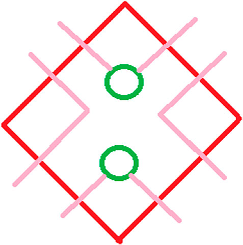
FIGURE 2. Resulting vertex after the integration over matrix B. The double pink lines indicate the propagator and the green circles indicate the insertion of the matrix C in the interaction.
We identify the matrix model action that implements CDT as
Which takes the form of the Euclidean action [25], except for the presence of matrix C. The appearance of the dual weighting matrix C changes the symmetry of the matrix model. Let us consider an N × N orthogonal matrix, O, and the transformation
Since the combination AAT is invariant A→OAant (14) is a symmetry of the Euclidean and the CDT action, however the conjugate symmetry under and AT→ATOT is only a symmetry of the Euclidean action and not of the CDT action. This shows an explicit difference with the real Euclidean matrix model. In the language of the renormalization group: the CDT action (13) lives in a different theory space, which is governed by a different symmetry.
Weighting Matrix
The matrix C implements the weighting of closed loops of propagators in the Feynman graph expansion, i.e. the dual weighting of the Feynman graphs. In principle one could define this matrix abstractly only through the property (8) and only use Eq. 8 whenever the matrix occurs in a Feynman diagram. However, in order to do practical calculations with the FRGE, it is very useful to have an explicit representation of C at ones disposal.
For a N × N diagonal matrix, X, with eigenvalues {xi} we can write its characteristic polynomial as
Where ek is
Then Newton identities allow us to write this coefficients in terms of the kth power of the trace of X, pk, in the form
So, C can be found by solving
These solutions exist by the fundamental theorem of algebra and one can use ones preferred approximation scheme to obtain these. One scheme that suggests itself in particular when one wants to gain insights into the effects of dual weightings is to build a matrix C from smaller blocks of matrices C0, so C = diag(C0,...,C0). The matrix obtained in this way does not implement the entire tower of Eq. 8, but permits traces periodically. This approach is particularly interesting to study, since it allows us to study how many of the equations one needs to enforce to attain the phase transition between the Euclidean matrix model and the CDT matrix model. The first three matrices CO are
Putting these together as blocks to build an N × N matrix gives for example for k = 2
And for k = 4
That are N × N matrices formed by 2 × 2 and 4 × 4 blocks, and where γ = 1.09 and ξ = 0.45.
Functional Renormalization Group for Matrix Models
Let us briefly review the application of the FRGE to matrix and tensor models. One can follow the fundamental presentation of [18] and apply it to matrix models as done in [23]. The starting point is the definition of the effective average action ГN[φ] in the presence of an IR-suppression term ΔSN[ϕ]:
Where
And φ represents the expectation value of a quantum field ϕ, while the term
Represents an IR-suppression term in so far as it is designed to give a mass term of order N to “IR” degrees of freedom of the matrix. Since matrix and tensor models do not implement a fundamental scale, there is no canonical identification of which degrees of freedom are “IR”. Rather one needs to implement by hand a division of theory space according to an RG scale k. The simplest assignment is to identify the upper-left corner of the matrix with index values below the scale k as “IR”. Once the IR-suppression term is chosen, one can proceed as in [18]; one arrives at the FRGE
Where t = 1nN. The solutions to (26) are functionals of the N × N matrix ϕ and hence of infinitely many degrees of freedom in the large N-limit. Practically one resorts to finite truncations of the effective average action, i.e. one performs an expansion of the effective average action into monomials
Then one truncates this expansion at a manageable set of operators
Which only includes operators with AAT, which is invariant under (14), and two C matrices. In the present contribution we will truncate this to the ansatz that contains the bare action and the single trace operator that can directly contribute to the beta functions of the bare action at one loop. This truncation is:
We introduce the dimensionless couplings
Where α4 and α6 are as of yet undetermined, since the matrix model does not include an intrinsic notion of scale. The scale is later fixed by imposing that the beta functions admit a 1/N expansion.
To make the calculation concrete, we choose the explicit form of the IR-suppression term RN to take the form
Which has the advantage of being a diagonal and field independent tensor, so we can readily invert the kinetic term to obtain the propagator. It is practically useful to split the second variation of the effective average action into a field independent term G and a field dependent term F:
Which allows us to expand the RHS of the Wetterich equation as a geometric series, using only the propagator P = G−1 and the F-term:
The upshot of this P−F expansion is that each F term contributes more field operators. Hence a truncation that contains polynomial operators with only a finite number of fields terminates the geometric series at a finite number of terms. With the proposed truncation (29), the first term in (33) is of order zero in the Feynman diagrams expansion since there is no field contribution, the second term gives rise to 2-vertex and 4-vertex diagrams which contribute to η and β4, the third one to 4-vertex and 6-vertex diagrams which contribute to β4 and β6 and so on.
2.5 Benchmark Results
We use the FRGE to find fixed points of the RG flow and to investigate the universality class associated with this fixed point. This is done by calculating the critical exponents θ at the fixed point, i.e. by considering the linearized FRGE-flow at the fixed point, where the critical exponents appear as the eigenvalues of the Hessian of the beta functions. We chose our truncation in such a way that we can resolve the fixed point that known as the double scaling limit in the matrix model literature. This fixed point possesses a single positive critical exponent, which is usually expressed in terms of the string susceptibility γstr:
For Euclidean Matrix Models [27] γstr = −1/2, while for CDT [28] γstr = +1/2, which leads to the following critical exponents
3 β-functions
In this section we summarize the steps that we took to obtain the beta functions of the matrix model for CDT.
3.1 Operator Products
The structure of the beta functions is determined by the operator products of the F-terms that we showed in (33). The terms FN(4) and FN(6) are the second variations of the operators whose contribution to the effective average action is measured by the coupling constants
And
By looking at (33), we notice that traces of products of (36) and 37 give rise to a big range of operators which are not present in the truncation ansatz (29), such as (Tr(CA))2, Tr(CAATC2)Tr(ATCA), etc. However, a reasonable projection rule onto the truncation should not project these operators onto the beta functions of the truncation. We therefore analyze which operators can contribute to the beta functions in the truncation, i.e. to β4 and β6. Considering for example the trace
We see that each term contains the matrix C, while we know from the structure of the P-F-expansion that these are the only terms generated by the restriction of the FRGE to the truncation that contain two matrices A. Hence, the restriction of the FRGE to the truncation does not generate terms ∼Tr(AAT) and hence does not generate any term that contributes to the anomalous dimension η. To generate a contribution to the anomalous dimension, one needed to include a term with a single C matrix in the truncation. This term would then be generated at one loop by the first term in (38) and in turn contribute to η at one loop. The investigation of this kind of secondary effect however goes beyond the scope of this first investigation.
This analysis relies on the fact that our projection rule is able to discern the structure in which the matrices A are contracted with the constant weighting matrix C, so at first sight one might worry that such a projection does not exist. However, one can consider the appearance of the matrix C in the operators as a special case of operators with index-dependence, i.e. operators whose variations w.r.t. A can not be expressed in terms of A and δij, which can be discerned by a suitable projection rule. Hence it is not only possible, but even prudent to use a projection rule that discerns the different ways in which the matrix C is contracted.
To make this distinction, we mark in the following the terms that contribute to the beta functions in our truncation by putting a box around them. Subsequently, we will impose the use of a projection rule that only retains these operators and thus consider only the contributions of the boxed terms.
When considering Tr((FN(4))n) with n > 2 we see that all resulting operators contain at least three C matrices which are not present in the original proposed action (29), this means that in this truncation the β-functions do not possess contributions coming from these traces.
3.2 General Form of the β-functions
Now that we have identified the terms that can contribute to the β-functions, we can write down the general structure of the beta functions. To do so, we introduce the constants Di, Ei and Fi, which depend on the details of the projection rule. Repeating the same argument as in the previous subsection for the single trace truncation 28 we obtain
For i odd
For i even
We can see in particular that in this truncation tadpoles and 2-vertex diagrams contribute.
4 Fixed Point Analysis and Scheme Dependence
By using the obtained general form of the beta functions for the single trace truncation at our disposal we can discuss fixed points. We first consider the fixed point structure analytically, before inserting particular truncation rules, which provide numerical values for the critical exponents, which allows us to discuss the scheme dependence of our calculation.
4.1 Analytic Fixed Point Analysis
By setting our truncation to (29), we obtain the following beta functions
Where η has been set to zero in accordance with our previous analysis. The set of fixed points of this system of beta functions is
And the Hessian matrix (defined as
Hence, the critical exponents, i.e. the eigenvalues of the Hessian, evaluated in each of the fixed points take the form.
The canonical dimensions α4 and α6 are not fixed by themselves, but tadpole diagrams show that α6 has to be one dimension of N greater than α4. We identify the Gaussian fixed point (0,0), which will not have a relevant direction. There are two non-Gaussian fixed points: the first fixed point (α4/E2,0) contains one relevant and one irrelevant direction if E2/E3 > α4/α6, and the third fixed point in Table 1 possesses a relevant and an irrelevant direction if E2/E3 < α4/α6. These two points are our candidates for a double scaling limit. Next we will examine them using particular schemes.
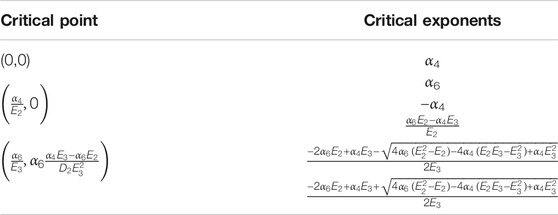
TABLE 1. Critical points with its corresponding pair of critical exponents.
4.2 Scheme Dependence
To find concrete critical exponents, we supplement the projection rule with the evaluation of both sides of the FRGE at preferred test matrices A. Moreover, we consider the two rigidity matrices obtained by constructing a block diagonal matrix from (18)(19), namely (21) and (19) respectively. The specific test matrices that we use for the projection are
Using three different matrices A allows us to estimate a lower bound for the scheme dependence. We expect this because the three field configurations contain two field configurations with distinct UV behavior and one manifest IR field configuration. One often assumes that the scheme dependence is an actual approximate measure for the quality of the fixed point analysis, however when comparing with analytic results, we will see that this underestimates the truncation error.
The corresponding obtained critical exponents are shown in Table 2 and the fixed points are shown in Table 3. The euclidean values are computed as done in [23] using (50), (51) and (52) as test fields.
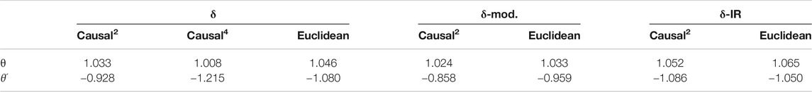
TABLE 2. Numerical values obtained for critical exponents. Causal2 corresponds to values computed using (21) and Causal4 corresponds to the ones computed using (LABEL:c4).
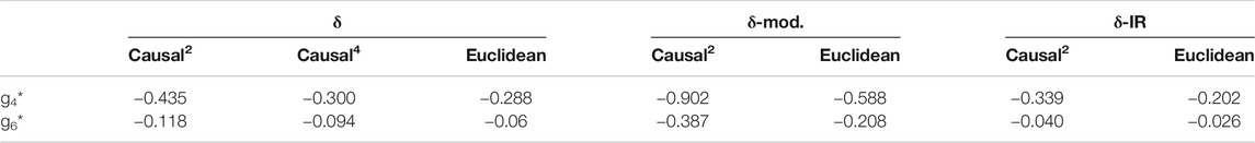
TABLE 3. Numerical values obtained for critical points. Causal2 corresponds to values computed using (21) and Causal4 corresponds to the ones computed using (LABEL:c4).
We see that the relevant critical exponents are all close to 1, while the irrelevant critical exponents spread a bit wider between −0.858 and −1.215. Moreover, we observe that all critical exponents lay within the spread obtained by scheme dependence. This means that we can not distinguish the Euclidean models from the Causal models, built from the 2 × 2 and 4 × 4 matrices, based on the present derivation of the critical exponents.
In order to attempt to obtain more accurate numerical values for the critical exponents we use the fixed point approximation. This consists in first finding the zeros of the beta functions, then evaluating the anomalous dimension, η, in the fixed point g4* and substituting this numerical value in the beta functions to find the critical exponents. The critical exponents obtained by using the fixed point approximation are shown in Table 4.
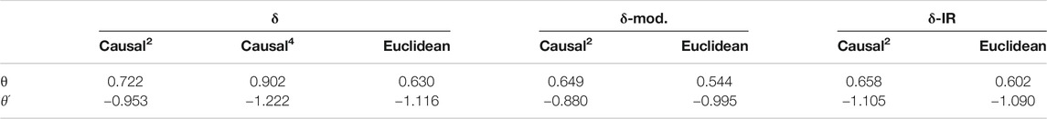
TABLE 4. Numerical values obtained for critical exponents using the fixed point approximation. Causal2 corresponds to values computed using (21) and Causal4 corresponds to the ones computed using (LABEL:c4).
Since the numerical values reported in Table 2 were found to have a strong scheme dependence, it is important to compare the renormalization scheme dependence vs. the causal-euclidean results in the latter ones in Table 4. We compute the average of the difference between the critical exponents obtained in the different renormalization schemes and the “Causal vs. Euclidean” results with each of both methods.
In Table 5 we observe that, while the first method (full) shows a stronger renormalization scheme dependence, with the fixed point approximation method the “Causal vs. Euclidean” relation is more significant than the renormalization scheme dependence. Regarding the accuracy of the values for the critical exponent obtained with both methods compared to the theoretical values (35), we observe that the Causal ones differ more from the theoretical value than the Euclidean critical exponents. Therefore we can conclude that in this case the fixed point approximation is more useful for differentiating the Causal from the Euclidean results, while the full method reproduces more accurate numerical results.
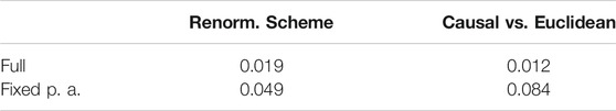
TABLE 5. Renormalization scheme dependence and Causal-Euclidean difference with both methods.
Conclusion
This contribution is motivated by the observation that the application of the FRGE to tensor models with dual weights could lead to an approach to quantum gravity that combines the advantages of the systematic search of continuum limits with the FRGE with the physically promising phase diagrams of CDT and EDT. The systematic development of these tools and the systematic investigation of these models is a very ambitious task. In this contribution we took a first step into this direction and considered the FRGE flow of a matrix model for CDT in 1 + 1 dimensions proposed by Benedetti and Henson. This model implements a foliation through a dual weighting of Feynman graphs, which introduces an action with an index-dependent propagator. This action, upon integration of an auxiliary field, reduces to an action with an index dependent interaction.
Recalling the critical exponents analysis in Analytic Fixed Point Analysis and the values in Table 1, we see that the model uses a rigidity matrix C which is chosen in such a way that one of the conditions for the beta function polynomials E2/E3 > α4/α6 or E2/E3 < α4/α6 is satisfied. In this case we obtain a relevant and an irrelevant direction simultaneously, implying that the only Feynman diagrams that contribute to the partition function are the ones where all C matrices are contracted as Tr(C2), which is precisely the condition that implements a foliation. In this contribution we considered a single trace truncation in which we included operators that contain two C-matrices with the pattern prescribed by the interaction in the Benedetti-Henson model and calculated the beta functions for this truncation. We found that wave function renormalization does not occur in this truncation, since the one-loop structure of the FRGE can only remove 1 C matrix. This technical observation has far reaching consequences for the structure of the beta functions, which change significantly compared to the Euclidean model, which is obtained by setting C to the identity matrix. In other words: the structure of the beta functions is more complicated and in particular includes wave function renormalization if C is replaced with the identity matrix.
We then investigated this system of beta functions in a truncation in which we included only a four- and a six-point interaction. Despite the significant difference in the structure of the beta functions, we found that this truncation contains fixed points that possess the properties of the double scaling limit. We investigated these fixed points numerically using three distinct field configurations for projection.
This numerical investigation revealed a practical challenge: To obtain numerical values for the beta functions one can not resort to an abstract definition of the rigidity matrix C, since the calculation requires an explicit numerical expression of C. We took this as an opportunity to investigate the weakening of the condition Tr(Cm) = δm mod k,2 for k = 2,4,6. This has the implication that not all Feynman diagrams without a foliation structure are suppressed, but only a part of these. In particular the case k = 2 does not introduce any new restriction at the level of Feynman diagrams of the Euclidean model, however, since we used the structure of the beta function for general C, we still obtained equations that differ from the Euclidean matrix model. The numerical investigations however revealed that we can not discern the Euclidean and the CDT model on the basis of the critical exponents at the fixed point associated with the double scaling limit. These results are summarized in Table 2. The obtained relevant critical exponent (θ) in the Benedetti-Henson model differs from the exact values in Benchmark Results by 0.31 from the CDT value and 0.27 from the Euclidean one. We also observe a 4% spread of these values depending on the field configuration used for projection, which is a significantly lower spread than the difference with the analytic values. This is however consistent with the results obtained in [23], where a similar difference from the analytic values was found. This was also to be expected, because the presented calculation is technically very similar to the calculation done in [23]. We therefore expect that the truncation error improves in a similar way as in [23] when the truncation is gradually increased. This means that we expect the truncation error to improve over the range of a few percent as one enlarges the truncation, but also that there will remain a significant deviation from the analytic results until the broken unitary Ward-Identity, stemming from the variation of the kinetic term, is solved in a self-consistent way.
We interpret our results as an encouragement for the investigation of dually weighted tensor models for quantum gravity: Already with the rather simple and elementary techniques used in this contribution we were able to investigate qualitatively the double scaling limit of the dually weighted matrix model; analogous dually weighted tensor models such as the one proposed in [22] can thus be treated with the FRGE in a similar fashion. Our results indicate some practical advise for these future investigations:
1) The one-loop structure of the FRGE can only couple effective operators that differ by an index-dependent contraction between two adjacent tensors, not more. Therefore, to study the influence of an operator with index-dependence in more than one contraction one needs to include sufficient “intermediary” operators in the truncation.
2) For analytical investigations it is possible to work with abstract rigidity structures, that are defined through its properties, such as Tr(Cm) = δm,2, however for numerical investigations one needs a projection onto the truncation and an explicit evaluation of the operator traces appearing on the RHS of the flow equation. This evaluation of the RHS requires an exact (or at least approximate) numerical representation of the abstract structure encoded in the rigidity matrix C. One might thus prefer the investigations of models for which one has one of these numerical representations at ones disposal.
3) If our present observations about the double scaling limit are transferable then one sees that the existence of a fixed point with certain characteristics can be found in rather small truncations. However, the critical exponents found in these truncations can be expected to differ significantly from the exact values (which of course should be accessible through lager truncations and optimized renormalization schemes).
These general observations can serve as a guide of what to expect in higher dimensions, where a modification of the propagator can be used to suppress the Feynman diagrams that lead to most significant deviations from foliated spacetimes. Unfortunately, our observations do not have an immediate implication for the existence of a physically viable continuum limit in higher dimensions.
A Recipe for Calculations
A detailed description of the recipe to do FRGE-calculations in matrix and tensor models has been presented in [24]. We essentially followed the recipe outlined there, but had to make some adjustments due to the appearance of the rigidity matrix C, which we present in the following.
A.1 Theory Space and Truncations
The theory space upon which we set up the flow equation must include the action proposed in [1] and thus include the rigidity matrix C. This action is invariant under the one-sided transformation A→AO, for all matrices OTO = 1. These actions can be expanded in terms of traces of products of ATA and C. It is useful to organize the trace operators systematically with increasing number of fields ATA. For a fixed number of fields we observe that
A.2 Canonical Dimension
The canonical dimension of the operators can be derived from the requirement that the beta functions possess a -expansion, since one could not use them to investigate the continuum limit if it were otherwise. The initial condition for this is that the couplings that appear in the bare action possess the same scaling as prescribed by the bare action proposed by Benedetti and Henson, where the regulator is chosen in such a way that it possesses the large N-scaling of the kinetic term. The vertex expansion of the beta functions then provides a set of inequalities that determines the scaling of the operators. The difference with the pure matrix model case is that the appearance of the rigidity matrix C appears on both sides of the flow equation, so that its influence on the scaling arguments has to be taken into account.
A.3 Projection and Extraction of Beta Functions
The most important adjustment to the recipe provided in [28] concerns the projection onto the truncation and the derivation of beta functions. The vertex expansion, the same as described in [28], provides a lot of structural insight into the beta functions, because it shows how operator traces can be converted into traces over products of ATA and C with the insertion of at most one regulator-dependent factor. These traces are not of the form of the operators that occur in the truncation, so one needs to find a projection onto the truncation. This is usually done by evaluating both sides of the FRGE on a family of field configurations that is large enough to distinguish all operators in the truncation, while one chooses them in such a way that the calculation is computationally feasible.
We have provided several families of field configurations that one can use to project onto the truncation, but this is not enough to evaluate both sides of the flow equation due to the appearance of the rigidity matrix C in the traces. In order to evaluate the traces, one needs an explicit expression of C in the presence of the regulator terms.
Author Contributions
All authors listed have made a substantial, direct, and intellectual contribution to the work and approved it for publication.
Conflict of Interest
The authors declare that the research was conducted in the absence of any commercial or financial relationships that could be construed as a potential conflict of interest.
Footnotes
1The term (un)-colored is explained in the next section.
References
1. Benedetti D, Henson J. Imposing causality on a matrix model. Phys Lett B (2009) 678:222–226. doi:10.1016/j.physletb.2009.06.027
2. Hawking SW, Israel W. General relativity: an einstein centenary survey. 1st ed. England, UK: Cambridge University Press (1979).
3. Donoghue JF. General relativity as an effective field theory: the leading quantum corrections. Phys Rev D (1994) 50:3874–3888. doi:10.1103/PhysRevD.50.3874
4. Reuter M. Nonperturbative evolution equation for quantum gravity. Phys Rev D (1998) 57:971–985. doi:10.1103/PhysRevD.57.971
5. Reuter M, Saueressig F. Quantum einstein gravity. New J Phys (2012) 14:055022. doi:10.1088/1367-2630/14/5/055022
6. Eichhorn A. An asymptotically safe guide to quantum gravity and matter. Front. Astron. Space Sci. (2019) 5:47. doi:10.3389/fspas.2018.00047
7. Thiemann T. Modern canonical quantum general relativity. England, United Kingdom: Cambridge University Press (2007).
8. Perez A. The spin-foam approach to quantum gravity. Living Rev Relativ (2013) 16:3. doi:10.12942/lrr-2013-3
9. Freidel L. Group field theory: an overview. Int J Theor Phys (2005) 44:1769–1783. doi:10.1007/s10773-005-8894-1
10. Rivasseau V. The tensor track: an update. Symmetries and Groups in Contemporary Physics. arXiv, 63–74. doi:10.1142/9789814518550_0011 CrossRef Full Text
12. Rivasseau V. Random tensors and quantum gravity. SIGMA (2016) 12:069. doi:10.3842/SIGMA.2016.069
13. Rivasseau V. Quantum gravity and renormalization: the tensor track. AIP Conf Proc (2012) 1444(1):18. doi:10.1063/1.4715396
14. Barceló C, Liberati S, Visser M. Analogue gravity. Living Rev. Relativ (2005) 8:12. doi:10.12942/lrr-2005-12
15. Witten E. Anti de Sitter space and holography. Adv Theor Math Phys (1998) 2:253–291. doi:10.4310/ATMP.1998.v2.n210.4310/atmp.1998.v2.n2.a2
16. Polchinski J. “An introduction to the bosonic string”, in String Theory. (1998) 1. doi:10.1017/CBO9780511816079
17. Ambjørn J, Görlich A, Jurkiewicz J, Loll R. Nonperturbative quantum de Sitter universe. Phys Rev D (2008) 78:063544. doi:10.1103/PhysRevD.78.063544
18. Wetterich C. Exact evolution equation for the effective potential. Phys Lett B (1993) 301:90–94. doi:10.1016/0370-2693(93)90726-X
19. Regge T. General relativity without coordinates. Nuovo Cim (1961) 19:558–571. doi:10.1007/BF02733251
20. Gurau R, Ryan JP. Melons are branched polymers. Ann Henri Poincaré (2014) 15:2085–2131. doi:10.1007/s00023-013-0291-3
21. Ambjorn J, Görlich A, Jurkiewicz J, Kreienbuehl A, Loll R. “Renormalization group flow in CDT,” class. Quant Grav (2014) 31:165003. doi:10.1088/0264-9381/31/16/165003
22. Benedetti D, Gurau R. Phase transition in dually weighted colored tensor models. Nucl Phys B (2012) 855:420–437. doi:10.1016/j.nuclphysb.2011.10.015
23. Eichhorn A, Koslowski T. Continuum limit in matrix models for quantum gravity from the functional renormalization group. Phys Rev D (2013) 88:084016. doi:10.1103/PhysRevD.88.084016
24. Gross M. Tensor models and simplicial quantum gravity in >2-D. Nucl Phys B - Proc Supplements (1992) 25:144–149. doi:10.1016/S0920-5632(05)80015-5
25. Eichhorn A, Koslowski T, Pereira A. Status of background-independent coarse graining in tensor models for quantum gravity. Universe (2019) 5(2):53. doi:10.3390/universe5020053
26. Eichhorn A, Koslowski T. Flowing to the continuum limit in tensor models for quantum gravity. Ann Inst Henri Poincaré Comb Phys Interact (2018) 5(2):173–210. doi:10.4171/AIHPD/52
27. Francesco PD, Ginsparg P, Zinn-Justin J. 2D gravity and random matrices. Phys Rep (1995) 254:133. doi:10.1016/0370-1573(94)00084-G
Keywords: matrix model, functional renormalization, causal dynamical triangulation, tensor model, continuum limit
Citation: Castro A and Koslowski TA (2021) Renormalization Group Approach to the Continuum Limit of Matrix Models of Quantum Gravity With Preferred Foliation. Front. Phys. 9:531766. doi: 10.3389/fphy.2021.531766
Received: 01 February 2020; Accepted: 16 February 2021;
Published: 16 April 2021.
Edited by:
Benjamin Bahr, University of Erlangen Nuremberg, GermanyReviewed by:
Sayantan Choudhury, National Institute of Science Education and Research (NISER), IndiaZhenbin Wu, University of Illinois at Chicago, United States
Copyright © 2021 Castro and Koslowski. This is an open-access article distributed under the terms of the Creative Commons Attribution License (CC BY). The use, distribution or reproduction in other forums is permitted, provided the original author(s) and the copyright owner(s) are credited and that the original publication in this journal is cited, in accordance with accepted academic practice. No use, distribution or reproduction is permitted which does not comply with these terms.
*Correspondence: Tim Andreas Koslowski, dC5hLmtvc2xvd3NraUBnbWFpbC5jb20=