 Biwei Zhang
 Jiazhu Zhu
 Ke Si1,2,3
 Wei Gong
- 1Department of Neurology of the Second Affiliated Hospital, State Key Laboratory of Modern Optical Instrumentation, Zhejiang University School of Medicine, Hangzhou, China
- 2College of Optical Science and Engineering, Zhejiang University, Hangzhou, China
- 3NHC and CAMS Key Laboratory of Medical Neurobiology, MOE Frontier Science Center for Brain Research and Brain–Machine Integration, School of Brain Science and Brain Medicine, Zhejiang University, Hangzhou, China
Deep learning (DL) has been recently applied to adaptive optics (AO) to correct optical aberrations rapidly in biomedical imaging. Here we propose a DL assisted zonal adaptive correction method to perform corrections of high degrees of freedom while maintaining the fast speed. With a trained DL neural network, the pattern on the correction device which is divided into multiple zone phase elements can be directly inferred from the aberration distorted point-spread function image in this method. The inference can be completed in 12.6 ms with the average mean square error 0.88 when 224 zones are used. The results show a good performance on aberrations of different complexities. Since no extra device is required, this method has potentials in deep tissue imaging and large volume imaging.
Introduction
Biomedical imaging often suffers from the optical aberrations caused by the highly scattering characteristic of the biological tissue [1]. As the imaging target goes deeper, more complex aberrations with increasing high-order components will come into existence because of the multiple scattering process, which may severely distort the imaging focus and thus greatly undermine the performance of deep tissue imaging [2]. Adaptive optics (AO) is one of the most common used techniques to correct the aberrations [3]. In this technique, the aberrations are directly measured by a wavefront sensor or detected in an indirect way, and then accordingly corrected by a spatial light modulator (SLM) or a deformable mirror (DM) [4]. Mostly, the pattern on the AO corrector needs to be inferred through a series of calculating operations [5,6] or multiple measurements [7–9]. As a result, the AO process can be time-consuming and therefore limits the imaging speed.
Recently, deep learning (DL) has been applied to find direct mapping relations by training neural networks on large datasets in various researches [10–13]. For the purpose of accelerating the AO process, there have also been works that take advantage of DL to simplify some conventional steps. Among these works, Hu et al. presented a learning-based Shark–Hartmann wavefront sensor (SHWS) to implement a fast AO with direct aberration measurement [14]. The Zernike coefficients controlling correction pattern were predicted by a revised AlexNet [15]—one of the most used DL networks—from a single SHWS pattern. Other works include Suárez Gómez et al. [16], Swanson et al. [17] and DuBose et al. [18]. Similar with most other direct AO methods, these work can be effectively adopted in retinal imaging [19] or to relatively transparent samples as zebrafish [20]. However, their further applications to most biological samples are inevitably limited by the fact that the SHWS can hardly be placed within the sample and the utilization of backscattered light is likely to lead highly degree of inaccuracy [21,22]. Since a large part of biological sample induced aberrations should be measured through an indirect way [9], DL assisted sensor-less AO techniques have been developed at the same time. One representative work was carried out by Paine et al. They trained an adapted Inception v3 network (another well-known DL network) to determine a desirable starting estimate for gradient-based wavefront optimization from the point-spread function (PSF) image so that less iterations were required to achieve convergence [23]. Jin et al. moved forward to generate the correction pattern directly from the AlexNet calculated Zernike coefficients with the PSF image as the input [24]. With this method, the time consumption caused by the iterations can be completely eliminated, so the running speed of these techniques got further promoted. However, because it will be increasingly difficult to implement the measurement as well as the correction precisely when the number of Zernike modes gets bigger, this modal AO approach is only able to correct low-order aberrations [25]. Though Cumming et al. predicted the aberration function instead of Zernike coefficients, it is still limited to correct simple aberrations of the first 14 Zernike polynomials [26]. Since high-order aberrations severely degrade a large proportion of biomedical imaging results [2], new AO method is needed to achieve the correction of more complex aberrations while keeping the fast speed.
In this article, we propose a DL assisted zonal adaptive correction (DLZAC) method. Instead of correcting aberrations by Zernike modes, we equally divide the distorted wavefront into a number of zones and correct the aberration in each zone independently. In this way, correction with much more degrees of freedom can be easily achieved with most local-element based active devices and thus deal with complex aberrations effectively. It is noted that this sort of zonal adaptive correction method has already been used in multiple researches to overcome complex aberrations from biomedical imaging. Some typical examples include the pupil-segmentation based AO method by Ji et al. [9] and multidither coherent optical adaptive technique by Liu et al. [25]. However, all these former methods require repeated measurements to decide how to correct different wavefront zones, and thereby slow down the speed by a large scale. Here we creatively utilize a revised ResNet-34 network [27] to infer the correction phases of all the 224 valid zones on a SLM from a single PSF image in one shot. With the acceleration of a graphic processing unit (GPU), the whole inference process can be even much faster than the DL assisted modal adaptive correction (DLMAC) method mentioned above [24]. We introduce complex aberrations by phase masks to test the inference accuracy of the network as well as the correction ability of our method. Furthermore, the performance of DLZAC is compared with that of DLMAC on aberrations of different complexities to demonstrate the superiority of our method.
Methods
Optical System
The optical system for DLZAC is illustrated in Figure 1A. In this system, a 488 nm wavelength laser beam is applied as the light source. Two lenses (L1 and L2) are located immediately after the source to serve as a beam expander. The pinhole (PH1) between L1 and L2 is used to collimate the beam. Then the expanded beam passes through a half-wave plate (HWP) and a polarized beam splitter (PBS) to adjust its power into an appropriate range. The PBS only allows horizontally polarized light to pass, so it also controls the beam polarization into the right state for SLM modulation together with a linear polarizer (P). After this, the beam is directed into a SLM for phase modulation. When the SLM is utilized for correction, it will be equally divided into 16 × 16 square zones with 224 of them is valid because of the round pupil. Each zone on the SLM is treated as one phase element to implement correction by a single ensemble phase. The SLM is further conjugated to the back-pupil plane of the objective (OBJ1) by two relay lenses (L3 and L4). Another pinhole is placed between the relay lenses to block out the unwanted diffraction light generated by SLM. When the modulated beam reaches the objective, it is then focused on the sample plane. In order to obtain the PSF image, here another objective (OBJ2) is straightly mounted on the other side of the focal plane for detection. The light collected by OBJ2 is finally focused by a lens (L5) and recorded by a CMOS camera.
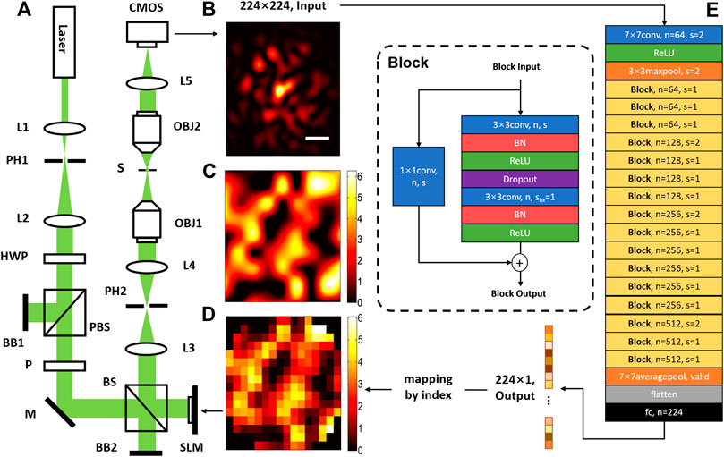
FIGURE 1. The schematic diagram of DLZAC. (A) An optical system for DLZAC: L1-L5, lens; PH1-PH2, pinhole; HWP, half-wave plate; PBS, polarized beam splitter; BB1-BB2, beam block; P, linear polarizer plate; M, mirror; BS, beam splitter, 50:50 (R:T); SLM(256 × 256), spatial light modulator; OBJ1-OBJ2, objective lens (Nikon, 20X/0.75 NA); S, sample plane; CMOS, complementary metal oxide semiconductor camera. (B) The 224 × 224 input PSF image (scale bar: 1 μm). (C) The phase mask. (D) The correction pattern. (E) The architecture of the DL network.
Deep Learning Network
To acquire the mapping relation between the PSF image and the zonal correction phases in DLZAC, the architecture of the neural network is correspondingly designed and shown in Figure 1E. To adapt the possible PSF of larger area as well as more complicated distribution induced by complex aberrations, the whole network architecture is based on ResNet-34, which is a powerful DL network with 34 weighted layers proposed by He et al. in 2016 [27]. The input of the network is a normalized 224 × 224 PSF image as shown in Figure 1B. The input size is set based on three considerations. First, the PSF should be covered as much as possible to minimize the margin feature loss; Second, the resolution of the PSF image should be as high as possible to minimize the fine feature loss; Third, the input size should be as small as possible to minimize the network computing cost. The network starts with a 7 × 7 convolutional layer of 64 kernels followed by a 3 × 3 max-pooling layer. Both of these two layers down-sampling the input by a stride of 2. Afterwards, the down-sampled feature maps are encoded by a series of layer blocks. In these blocks, the block input is filtered by two stacked 3 × 3 convolutional layers. Batch Normalization (BN) is adopted on both of the two convolutional layers before the activation and dropout is used after the first convolutional layer. To obtain the final block output, a special shortcut connection is implemented on every block by adding the block input to the output of the last block layer in an element-wise manner channel by channel. To make sure that the input dimension matches the dimension of the output, a 1 × 1 convolutional layer is used to operate the input before the addition. There are 16 blocks in total which can be further divided into four sequential groups by the channel number. The four groups consist of three blocks with 64 channels, four blocks with 128 channels, six blocks with 256 channels and three blocks with 512 channels respectively. It is noted that every time when the channel number doubles, the size of feature maps is halved to keep the time complexity. The output of the last block is further converted into a vector by a 7 × 7 average-pooling layer without padding. At the end of the network, a fully-connected layer is applied to perform a 224-variable regression. In the whole network, the activation is realized by Rectified Linear Unit (ReLU) function and padding is used to preserve the size of each layer with default stride as one if not specified. Finally, the network output is a 224 × 1 vector, of which each element corresponds to the correction phase of a fixed index SLM zone. Compared with AlexNet previously used by DLMAC, this revised ResNet-34 possesses larger depth and complexity, hence the high-level features brought by high-order aberrations can be better extracted and the correction phases are likely to be deduced more accurately. The possible degradation problem of deeper network is addressed by the shortcut connections in ResNet-34, which further ensure the superiority. Moreover, this revised ResNet-34 has significantly lower time complexity than most other deep networks so that the fast speed of DLZAC can be guaranteed.
To support the supervised learning of the network, datasets containing 220 thousand input-output pairs are built for training and testing [28–30]. In order to prepare these datasets, a large number of phase masks as shown in Figure 1C are randomly generated and added on the SLM respectively to introduce different aberrations. To make these phase masks fluctuate with a certain local smoothness, which is a common characteristic of actual aberration-distorted wavefront, we down-sample every phase mask before assign a random phase value between 0 and 2π to each pixel of it and then restore the original size by bicubic interpolation during the generation. According to different phase masks, corresponding PSF images can be obtained from the CMOS as the input part of the datasets. To get the reference zonal correction phases for the output vectors, we calculate the ensemble phase by vector averaging the phases of all the pixels within each SLM zone on every phase mask and arrange them by zone index. Finally, by matching each input with its corresponding output to form pairs, the datasets preparation can be accomplished.
For the training of the network, we allocate 200 thousand data as the training set and 10 thousand data for validation. Owing to the regression task, the loss is defined by mean square error (MSE). An L2 regularization term with the coefficient being 0.002 is further added on the loss to avoid the overfitting. To realize the training, the network weights are initialized by Xavier initialization and then trained for 200 epochs. We use Adam for optimization during the training with a mini-batch size of 32. To improve the training efficiency, the learning rate (LR) is decayed to 0.8 times of its former value every 10 epochs from 0.0001. The dropout ratio is set to 0.5 for the whole training process. To implement the network training, we apply Tensorflow framework (GPU version 1.12.0) based on Python 3.6.8 on a personal computer (PC, Intel Core i7 4770K 3.50 GHz, Kingston 16GB, NVIDIA GeForce GTX970).
Workflow of DLZAC
With the optical system presented in Figure 1A as well as the well-trained DL network mentioned above, the workflow of DLZAC can be divided into four steps. First of all, the distorted PSF is caused by a given aberration and recorded by the CMOS. Secondly, the PSF image from the CMOS is cropped and fed into the trained DL network to calculate the output by forward propagation. Thirdly, the output, namely the 224-element zonal correction phase vector, is mapped to a correction pattern as shown in Figure 1D by the index of SLM zones. Finally, the correction pattern is loaded onto the SLM to perform adaptive correction. In this way, DLZAC is capable of the fast correction of complex aberrations.
Results
The DLZAC performance largely depends on the inference accuracy of zonal correction phases. Figure 2A gives the descent curve of MSE on the training set as well as the validation set during the overall training process. The inset at the upper right corner shows the LR variation as the number of epochs increases. It can be seen that MSE on both datasets has been lower than 1.0 without obvious overfitting after the training of 200 epochs. To test the inference accuracy of the trained network, here we use the leftover 10 thousand data as the test set. Figure 2B presents the ideal correction phase pattern of an example in the test set. The pattern predicted by the trained network from the input PSF image corresponding to Figure 2B is displayed in Figure 2C. By comparison between these two patterns, we can find that they are in good agreement despite some tolerable differences. The phase differences are shown in Figure 2D with a white circle used to mark out the border of the pupil. It is obvious that the average difference of all the SLM zones within the pupil is quite small. Furthermore, we plot the phase difference of each zone in a bar chart shown in Figure 2E. It is easy to observe from the chart that most of the differences are around 0, which means a good accuracy of the network inference. The standard deviation σ of all the differences in Figure 2E is computed to be 0.78. It is noted from the figures that the comparatively obvious errors tend to appear at the locations where there are phase jumps among adjacent zones. After implementing tests throughout the whole set, we calculate the mean MSE to be 0.88. The time cost of a single test is 12.6 ms on average based on the PC we previously utilized for the training. These results demonstrate that the proposed method is able to deduce the correction patterns with desirable precision in a rather fast speed.
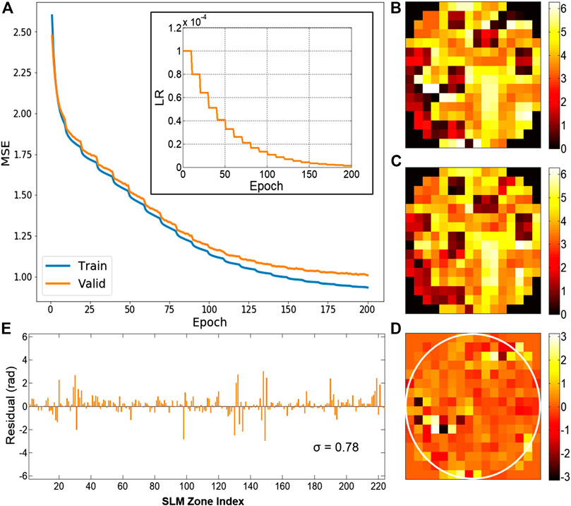
FIGURE 2. (A) The descent curve of MSE during the training process. Subfigure: the LR decay curve. (B) The ideal correction phase pattern. (C) The phase pattern predicted by the trained network. (D) The phase difference pattern between (B) and (C). (E) The bar chart of the phase difference on every SLM zone from (D), with the standard deviation σ being 0.78.
In order to verify the ability of DLZAC to correct aberrations, we randomly choose six examples from the test set and compare the PSFs before and after DLZAC. In Figure 3, each column corresponds to one of the six examples. The distorted PSFs before the correction are presented in the first row of Figure 3. It can be seen that these PSFs are severely distorted by complex aberrations. Here we introduce focal intensity ratio (FIR) as an indicator to quantify the distortion level of PSFs. The FIR is defined as the ratio between the intensity calculus within the Airy disk radius of the distorted PSF and that of ideal PSF with no distortion. All the six chosen PSFs are with a FIR below 0.34, which means that at least two-thirds of the light is scattered out of the focal area in these PSFs because of the complex aberrations. The second row of Figure 3 gives the corrected PSFs after DLZAC. Obviously, all the distorted PSFs are recovered to approximate diffraction-limited state, which represents that DLZAC is reliable on complex aberration correction. The third row of Figure 3 shows the phase wavefronts before DLZAC of the examples. The fourth row of Figure 3 shows the residual phase wavefronts within the pupil of the six test examples after DLZAC. The residual phase wavefront is obtained by adding the correction phase pattern to the phase mask. It can be observed that these corrected wavefronts all have fairly good flatness, which further demonstrates that the complex aberrations can be well compensated by our newly proposed AO method. To support our results quantitatively, we calculate and summarize the FIR of the PSFs before and after DLZAC in Figure 3E. Every FIR has enhanced significantly to about twice of its former value because of the highly effective correction.
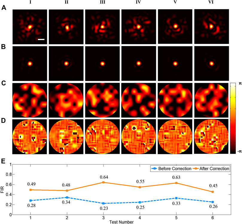
FIGURE 3. (A) The six distorted PSFs before correction (scale bar: 1 μm). (B) The six corrected PSFs after DLZAC. (C) The six phase wavefronts before DLZAC. (D) The six residual phase wavefronts within the pupil after DLZAC. Each column of (A–D) corresponds to one of the six test examples. (E) The FIR statistics of the PSFs in (A) and (B).
For the purpose of comparing the correction effect of our DLZAC with that of DLMAC on aberrations of different complexities, here we produce four kinds of aberrations by phase masks to control the FIR of distorted PSFs to form a gradient. In Figure 4, the distorted PSFs are shown in descending order of FIR from the top to the bottom of the first column, with each row corresponding to a kind of aberration complexity. It can be easily observed that the distortion extent of these PSFs is gradually increased as the FIR drops from 0.6 to 0.1. When the FIR of the distorted PSF equals 0.6, we can notice from Figure 4A1 that the aberration is relatively simple. Figures 4A2,3 display the corrected PSFs after DLMAC and DLZAC respectively. Apparently, both of the two methods have a certain effect of correction, while DLZAC achieves a better performance. We further calculate the FIR of two corrected PSFs. The FIR of DLZAC equals 0.83, which is much higher than that of DLMAC being 0.65. To compare different PSFs more intuitively, we plot the intensity profiles along the white dashed lines representing the central axis shown in Figures 4A1–3 and gather them in Figure 4A4. The red dashed line shown in Figure 4A4 gives the profile of the ideal PSF. It can be seen here that the two profiles belonging to the corrected PSFs have higher peak than that of distorted PSF and the profile corresponding to DLZAC is closer to the ideal profile than that of DLMAC. Based on these results, we can prove the fact that DLZAC is able to correct simple aberrations better than DLMAC. Afterwards, we then conduct DLMAC as well as DLZAC on the other three distorted PSFs of lower FIR. Since more complex aberrations need to be corrected in these circumstances, it is easy to tell from the comparisons between Figures 4B1,2,C1,2,D1,2 that the PSFs remain distinctly distorted after DLMAC. On the other hand, we can see from Figures 4B3,C3,D3 that the PSFs can still be recovered to a degree of satisfaction after DLZAC. Even to the highly distorted PSF with multiple peaks presented in Figure 4D1, DLZAC can still successfully enhance the FIR to 0.5. Similarly, we compare different PSFs by intensity profile along the central axis in Figures 4B4,C4,D4. It can be seen that the profiles of DLZAC in these three figures all have much more desirable shape and higher peak, whereas basically no improvement can be found in the profiles of DLMAC, compared to the distorted profiles. Therefore, it is verified that DLZAC can keep its remarkable correction performance, while DLMAC loses its correction effect with regard to complex aberrations.
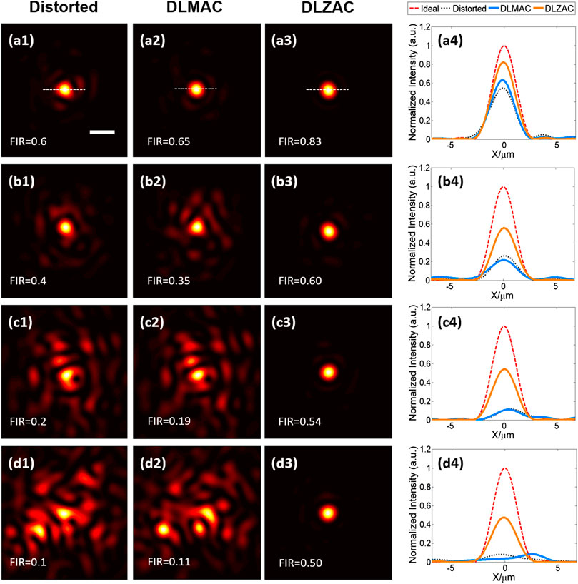
FIGURE 4. (A1) The distorted PSF whose FIR equals 0.6 (scale bar: 1 μm). (A2) The corrected PSF from (A1) by DLMAC. (A3) The corrected PSF from (A1) by DLZAC. (A4) The intensity profiles along the white dashed lines in (A1–3), with an extra profile of the ideal PSF. (B1–4) The equivalents of (A1–4) when the FIR of the distorted PSF equals 0.4. (C1–4) The equivalents of (A1–4) when the FIR of the distorted PSF equals 0.2. (D1–4) The equivalents of (A1–4) when the FIR of the distorted PSF equals 0.1.
Discussion
We present a DLZAC method in this article to achieve complex aberration AO correction for biomedical imaging in fast speed. Since the previous DLMAC method can only work on low-order simple aberrations, our method successfully overcomes this restriction by conducting the aberration measurement as well as the correction in a zonal way. To implement our method, we train a revised ResNet-34 network to infer the vector of 224 zonal correction phases from the PSF image and realize the correction by a SLM. With the acceleration of a GPU, the inference can be finished in 12.6 ms, which is even much faster than DLMAC, merely on a PC (Intel Core i7 4770K 3.50 GHz, Kingston 16 GB, NVIDIA GeForce GTX970) with the average MSE being 0.88. As for complex aberrations introduced by phase masks, which severely distort the PSF, DLZAC can recover the distorted PSF to near diffraction-limited state and significantly enhance the FIR. Compared with DLMAC, DLZAC presents even better correction on relatively simple aberrations. When the aberrations become highly complex and far beyond the correction capacity of DLMAC, DLZAC can still preserve its desirable correction performance. Since no extra device is required to implement DLZAC, our method is highly compatible with most of existing AO systems for biomedical imaging. The outstanding correction effect of kinds of aberrations, especially complex aberrations, makes DLZAC able to applied on a large range of imaging tasks. For deep living tissue imaging, DLZAC can bring benefits to remove dynamic complex aberrations caused by tissue movements and optimize the imaging result. Besides, with the rapid correction speed, DLZAC can also help to obtain the high imaging quality while keeping the efficiency as well as the photodamage level of large volume imaging.
Data Availability Statement
The original contributions presented in the study are included in the article, further inquiries can be directed to the corresponding author.
Author Contributions
BZ conceived the idea, did the simulation. JZ did additional experiments and data analysis. KS and WG supervised the project. BZ, JZ, KS, and WG wrote the paper. All the authors contributed to the discussion on the results for this manuscript.
Funding
National Natural Science Foundation of China (61735016, 81771877, 61975178); Natural Science Foundation of Zhejiang Province (LZ17F050001).
Conflict of Interest
The authors declare that the research was conducted in the absence of any commercial or financial relationships that could be construed as a potential conflict of interest.
References
1. Ji N. Adaptive optical fluorescence microscopy. Nat. Methods (2017) 14:374–80. doi:10.1038/nmeth.4218
3. Booth M. Adaptive optical microscopy: the ongoing quest for a perfect image. Light Sci. Appl. (2014) 3:e165. doi:10.1038/lsa.2014.46
4. Booth M. Adaptive optics in microscopy. Philos. Trans. Ser. A. Math. Phys. Eng. Sci. (2008) 365:2829–43. doi:10.1098/rsta.2007.0013
5. Cha JW, Ballesta J, So PTC. Shack-Hartmann wavefront-sensor-based adaptive optics system for multiphoton microscopy. J. Biomed. Optic. (2010) 15(4):046022. doi:10.1117/1.3475954
6. Tao X, Azucena O, Fu M, Zuo Y, Chen D, Kubby J. Adaptive optics microscopy with direct wavefront sensing using fluorescent protein guide stars. Opt. Lett. (2011) 36:3389–91. doi:10.1364/OL.36.003389
7. Sherman L, Ye JY, Albert O, Norris TB. Adaptive correction of depth-induced aberrations in multiphoton scanning microscopy using a deformable mirror. J. Microsc. (2002) 206(1):65–71. doi:10.1046/j.1365-2818.2002.01004.x
8. Marsh P, Burns D, Girkin J. Practical implementation of adaptive optics in multiphoton microscopy. Opt. Exp. (2003) 11:1123–30. doi:10.1364/OE.11.001123
9. Ji N, Milkie D, Betzig E. Adaptive optics via pupil segmentation for high-resolution imaging in biological tissues. Nat. Methods (2010) 7:141–7. doi:10.1038/nmeth.1411
10. Schmidhuber J. Deep learning in neural networks: an overview. Neural Netw. (2015) 61:85–117. doi:10.1016/j.neunet.2014.09.003
11. Guo Y, Liu Y, Oerlemans A, Lao S, Wu S, Lew MS. Deep learning for visual understanding: a review. Neurocomputing (2016) 187:27–48. doi:10.1016/j.neucom.2015.09.116
12. Min S, Lee B, Yoon S. Deep learning in bioinformatics. Briefings Bioinf. (2016) 18(5):851–69. doi:10.1093/bib/bbw068
13. Barbastathis G, Ozcan A, Situ G. On the use of deep learning for computational imaging. Optica (2019) 6:921–43. doi:10.1364/OPTICA.6.000921
14. Hu L, Hu S, Gong W, Si K. Learning-based Shack-Hartmann wavefront sensor for high-order aberration detection. Opt. Exp. (2019) 27:33504. doi:10.1364/OE.27.033504
15. Krizhevsky A, Sutskever I, Hinton GE. ImageNet classification with deep convolutional neural networks. Commun ACM (2017) 60(6):84–90. doi:10.1145/3065386
16.SL Suárez Gómez, C González-Gutiérrez, E Díez Alonso, JD Santos Rodríguez, ML Sánchez Rodríguez, J Carballido Landeiraet al. editors. Improving adaptive optics reconstructions with a deep learning approach. Cham: Springer (2018).
17. Swanson R, Kutulakos K, Sivanandam S, Lamb M, Correia C. Wavefront reconstruction and prediction with convolutional neural networks. Washington, DC: OSA Publishing (2018). p 52.
18. DuBose TB, Gardner DF, Watnik AT. Intensity-enhanced deep network wavefront reconstruction in Shack–Hartmann sensors. Opt. Lett. (2020) 45(7):1699–702. doi:10.1364/OL.389895
19. Porter J, Awwal A, Lin J, Queener H, Thorn K. Adaptive optics for vision science: principles, practices, design and applications. New York, NY: Wiley (2006).
20. Wang K, Sun W, Richie C, Harvey B, Betzig E, Ji N. Direct wavefront sensing for high-resolution in vivo imaging in scattering tissue. Nat. Commun. (2015) 6:7276. doi:10.1038/ncomms8276
21. Liang J, Williams D, Miller D. Supernormal vision and high-resolution retinal imaging through adaptive optics. J. Opt. Soc. Am. A Opt. Image Sci. Vision (1997) 14:2884–92. doi:10.1364/JOSAA.14.002884
22. Rückel M, Mack-Bucher J, Denk W. Adaptive wavefront correction in two-photon microscopy using Coherence-Gated Wavefront Sensing. Proc. Natl. Acad. Sci. USA. (2006) 103:17137–42. doi:10.1073/pnas.0604791103
23. Paine S, Fienup J. Machine learning for improved image-based wavefront sensing. Opt. Lett. (2018) 43:1235. doi:10.1364/OL.43.001235
24. Jin Y, Zhang Y, Hu L, Huang H, Xu Q, Zhu X, et al. Machine learning guided rapid focusing with sensor-less aberration corrections. Opt. Exp. (2018) 26:30162. doi:10.1364/OE.26.030162
25. Liu R, Milkie D, Kerlin A, Maclennan B, Ji N. Direct phase measurement in zonal wavefront reconstruction using multidither coherent optical adaptive technique. Opt. Exp. (2014) 22:1619–28. doi:10.1364/OE.22.001619
26. Cumming BP, Gu M. Direct determination of aberration functions in microscopy by an artificial neural network. Opt. Exp. (2020) 28(10):14511–21. doi:10.1364/OE.390856
27. He K, Zhang X, Ren S, Sun J. Deep residual learning for image recognition. CVPR (2016) 770–8. doi:10.1109/CVPR.2016.90
28. Cheng S, Li H, Luo Y, Zheng Y, Lai P. Artificial intelligence-assisted light control and computational imaging through scattering media. J. Innov. Opt. Health Sci. (2019) 12(04):1930006. doi:10.1142/s1793545819300064
29. Luo Y, Yan S, Li H, Lai P, Zheng Y. Focusing light through scattering media by reinforced hybrid algorithms. APL Photonics (2020) 5(1):016109. doi:10.1063/1.5131181
Keywords: deep learning, microscopy, biomedical imaging, aberration correction, deep tissue focusing
Citation: Zhang B, Zhu J, Si K and Gong W (2021) Deep Learning Assisted Zonal Adaptive Aberration Correction. Front. Phys. 8:621966. doi: 10.3389/fphy.2020.621966
Received: 27 October 2020; Accepted: 03 December 2020;
Published: 14 January 2021.
Edited by:
Ming Lei, Xi’an Jiaotong University, ChinaReviewed by:
Puxiang Lai, Hong Kong Polytechnic University, Hong KongHui Li, Suzhou Institute of Biomedical Engineering and Technology (CAS), China
Copyright © 2021 Zhang, Zhu, Si and Gong. This is an open-access article distributed under the terms of the Creative Commons Attribution License (CC BY). The use, distribution or reproduction in other forums is permitted, provided the original author(s) and the copyright owner(s) are credited and that the original publication in this journal is cited, in accordance with accepted academic practice. No use, distribution or reproduction is permitted which does not comply with these terms.
*Correspondence: Wei Gong, d2VpZ29uZ0B6anUuZWR1LmNu