95% of researchers rate our articles as excellent or good
Learn more about the work of our research integrity team to safeguard the quality of each article we publish.
Find out more
REVIEW article
Front. Phys. , 10 December 2020
Sec. Interdisciplinary Physics
Volume 8 - 2020 | https://doi.org/10.3389/fphy.2020.604053
This article is part of the Research Topic The Fiber Bundle View all 12 articles
The statistical distribution of the largest value drawn from a sample of a given size has only three possible shapes: it is either a Weibull, a Fréchet or a Gumbel extreme value distributions. I describe in this short review how to relate the statistical distribution followed by the numbers in the sample to the associate extreme value distribution followed by the largest value within the sample. Nothing I present here is new. However, from experience, I have found that a simple, short and compact guide on this matter written for the physics community is missing.
Extreme value statistics offers a powerful tool box for the theoretical physicist. But it is the kind of tool box that is not missed before one has been introduced to it—perhaps a little like the smart phone. It concerns the statistics of extreme events and it aims to answer questions like “if the strongest signal I have observed over the last hour had the value x, what would the strongest signal expected to be if measured over hundred hours?” Furthermore, if I divide up this hundred-hour interval into a hundred 1-h intervals, what would be the statistical distribution of strongest signal in each 1-h interval?
It is the latter question which is the focus of this mini-review.
There is no lack of literature on extreme value statistics, see e.g., [1–5] or simply google the term. We find it used in connection with spin glasses and disordered systems [6], in connection with
So, there is no lack of material for the novice that has seen a need for this tool. The problem is that it is not so easy to penetrate the literature, which is often cast in a rather mathematical language which takes work to penetrate. The aim of this mini-review is to present the theory behind and the main results concerning the extreme value distributions in a simple and compact way. We will present nothing new. For a longer, wider and more detailed review of extreme value statistics, Fortin and Clusel [12] or Majumdar et al. present exactly that [13].We have a statistical distribution
which is the probability to find a number smaller than or equal to x. We draw N numbers from this distribution and record the largest of the N numbers. We repeat this procedure M times and thereby obtain M largest numbers, one for each sequence. What is the distribution of these M largest numbers in the limit when
It turns out that depending on
• The Weibull cumulative probability
where we assume
• The Fréchet cumulative probability
Also here we assume
• The Gumbel cumulative probability
where
The questions are 1. which classes of distributions
• distributions where
• distributions where
• and distributions where
Furthermore, we will find that.
• for the Weibull extreme value distribution, u is given in terms of x in Eq. 13,
• for the Fréchet extreme value distribution, u given in terms of x in Eq. 27,
• for the Gumbel extreme value distribution, u is given in terms of x in Eqs 51 and 43.
We summarize these results in Table I.
The discussion that will now follow, will be built on the following relation. We draw N numbers from the probability distribution
where
Rather than the conventional approach (see e.g., [10]) to this subject based on the Fréchet, Fisher and Tippett stability criterion [1], I will base the entire discussion on the relation
I believe this to be the simpler and more intuitive way.
We consider here probability distributions
where b is positive. We note that
The extreme value cumulative probability for N samplings is given by
for
where the reader should note that b is defined by the original distribution 10. Equation 12 then becomes
In the limit of
for negative u. Hence, we have that
which is the Weibull cumulative probability, valid for all values of u even though we only know the behavior of
We note that the Weibull distribution resembles a stretched exponential. This is correct for
We express the Weibull cumulative probability in terms of the original variable x using Eq. 13,
Hence, in terms of the original variable x, the Weibull extreme value distribution becomes
We now work out a concrete example. Let us assume that
i.e.,
From Eq. 19 and we have that
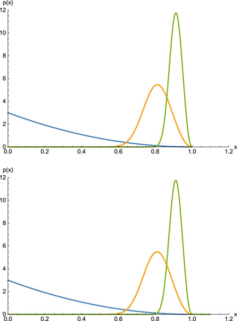
We show the distribution 20 with

FIGURE 1. (A) The curve that has its maximum at
Using a random number generator producing IID numbers1r uniformly distributed on the unit interval, we may stochastically generate numbers that are distributed according to the probability density
where we have also used that r may be substituted for
The Weibull distribution, Eq. 17 is much used in connection with material strength [15]. This is no coincidence. Consider a chain. Each link in the chain can sustain a load up to a certain value, above which it fails. This maximum value is distributed according to some probability distribution. When the chain is loaded, it will be the link with the smallest failure threshold that will break first causing the chain as a whole to fail. Hence, the strength distribution of an ensemble of chains is an extreme value distribution, but with respect to the smallest rather than the largest value. The link strength must a positive number. Hence, the link strength distribution is cut off at zero or some positive value. The distribution close to this cutoff value must behave as a power law in the distance to the cutoff, e.g., due to a Taylor expansion around the cutoff. The corresponding extreme value distribution, which is the chain strength distribution, must then be a Weibull distribution.
We now assume that the probability distribution
and the corresponding cumulative probability behaves as
The extreme value cumulative probability for N samplings is given by
for
where b comes from the original distribution 24. We now plug this change of variables into Eq. 26 to find
In the limit of
where
which is the Fréchet cumulative probability. The Fréchet probability density is given by
We express the Fréchet cumulative probability in terms of the original variable x using Eq. 27,
Hence, in terms of the original variable x, the Fréchet extreme value distribution becomes
We consider the distribution
The corresponding cumulative probability is given by
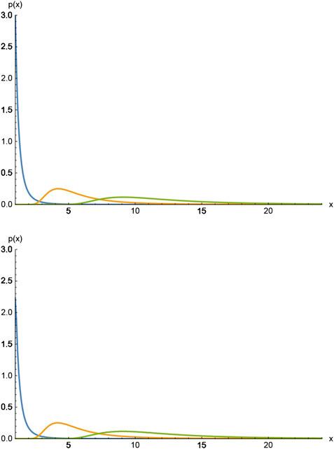
Using Eq. 33, we find the corresponding Fréchet extreme value distribution to be
valid for all

FIGURE 2. (A) The curve that has its maximum at
In order to compare with numerical results, we generate numbers distributed according to 34 by solving the equation
We generate a sequence of numbers using this algorithm, grouping them together in sequences of
We now assume we have a probability distribution that takes the form
where
This criterion is e.g., fulfilled by any polynomial
The cumulative probability is
We do not care about the form of
The extreme value cumulative probability for N samplings is given by
for
where
Even though
Let us now define
We then expand
where
so that the first order term in the expansion becomes constant as N increases, we will have that
Hence, if we have that
for
where we define
Here we have used Eqs (40) and (44).
If we combine Eq. 49 for
which is equivalent to
Equation 53, which is equivalent to Eq. 39, is in fact a sufficient condition for 49 to hold for all
If condition 52 is fulfilled, that is when the expression above is zero in the limit
since both terms on the right hand side of Eq. 54 are zero in this limit. We now assume Eq. 49 to be true for some
again due to both terms on the right hand side of Eq. 54 are zero in this limit. This completes the proof.
We now combine Eq. 42 with Eq. 41 to find
In the limit of
which is the Gumbel cumulative probability. Here
We express the Gumbel cumulative probability in terms of the original variable x using Eq. 51,
Hence, in terms of the original variable x, the Gumbel extreme value distribution becomes
Here is an example: the Gaussian. The Gaussian probability density is given by
where σ is the square of the standard deviation. The cumulative probability is
where
The Gaussian cumulative probability in Eq. 63 has the asymptotic form
for large x. We determine
where
when inserting the expression for
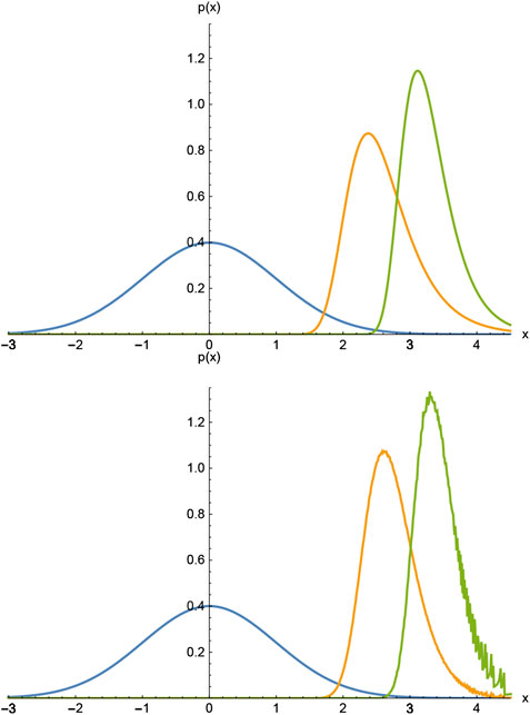
We show in Figure 3A the Gaussian and the corresponding Gumbel distributions for

FIGURE 3. (A) The Gaussian and the corresponding Gumbel distributions for
We show in Figure 3B a histogram based on numbers distributed according to a Gaussian distribution using the Box-Müller algorithm [14]. These numbers were grouped together in sets of either
We summarize the main results presented in this mini-review in Table I.
We have only discussed the distributions associated with the largest values of x except for the Weibull extreme value distribution, Section 2. It is, however, easy to work out: just transform
There is one remark that needs to be made, though. In the derivation of the Gumbel extreme value distribution, Section 4, we defined a variable
The probability density for the largest among N numbers drawn using the probability distribution
We calculate the average of the cumulative probability
For large N, we may write this as
using here Eq. 43. Hence, we may interpret
The author confirms being the sole contributor of this work and has approved it for publication.
This work was partly supported by the Research Council of Norway through its Centers of Excellence funding scheme, project number 262644.
The author declares that the research was conducted in the absence of any commercial or financial relationships that could be constructed as a potential conflict of interest.
I thank Eivind Bering, Astrid de Wijn, H. George, E. Hentschel, Srutarshi Pradhan, and Itamar Procaccia for numerous interesting discussions on this topic.
IID variables. Independent and identically distributed random variables, a terminology used in some communities.
4. Embrechts P, Klüppelberg C, Mikosh T. Modeling extreme events for insurance and finance. Berlin: Springer(1997).
6. Bouchaud J-P, Mézard M. Universality classes for extreme-value statistics. J Phys Math Gen(1997). 30:7997. doi:10.1088/0305-4470/30/23/004
7. Antal T, Droz M, Györgyi G, Rácz Z. 1/f noise and extreme value statistics. Phys Rev Lett(2001). 87:240601. doi:10.1103/physrevlett.87.240601
8. Randoux S, Suret P. Experimental evidence of extreme value statistics in Raman fiber lasers. Opt Lett(2012). 37:500. doi:10.1364/OL.37.000500
9. Taloni A, Vodret M, Costantini G, Zapperi S. Size effects on the fracture of microscale and nanoscale materials. Nat Rev Mater(2018). 3:211–24. doi:10.1038/s41578-018-0029-4
11. Pal A, Eliazar I, Reuveni S. First passage under restart with branching. Phys Rev Lett(2019). 122:020602. doi:10.1103/PhysRevLett.122.020602
12. Fortin J-Y, Clusel M. Applications of extreme value statistics in physics. J Phys Math Theor(2015). 48:183001. doi:10.1088/1751-8113/48/18/183001
13. Majumdar SN, Pal A, Schehr G. Extreme value statistics of correlated random variables: a pedagogical review. Phys Rep (2020) 840:1. doi:10.1016/j.physrep.2019.10.005
14. Press WH, Teukolsky SA, Vetterling WT, Flannery BP. Numerical recipes. 3rd ed. Cambridge: Cambridge University Press(2007).
16. Corless RM, Gonnet GH, Hare DEG, Jeffrey DJ, Knuth DE. On the LambertW function. Adv Comput Math (1996) 5:329–59. doi:10.1007/BF02124750
Keywords: extreme value statistics, statistical analysis, Weibull analysis, Gumbel distribution, Frechet distribution, Weibull distribution
Citation: Hansen A (2020) The Three Extreme Value Distributions: An Introductory Review. Front. Phys. 8:604053. doi: 10.3389/fphy.2020.604053
Received: 08 September 2020; Accepted: 22 October 2020;
Published: 10 December 2020.
Edited by:
Matjaž Perc, University of Maribor, SloveniaReviewed by:
Arnab Pal, Tel Aviv University, IsraelCopyright © 2020 Hansen. This is an open-access article distributed under the terms of the Creative Commons Attribution License (CC BY). The use, distribution or reproduction in other forums is permitted, provided the original author(s) and the copyright owner(s) are credited and that the original publication in this journal is cited, in accordance with accepted academic practice. No use, distribution or reproduction is permitted which does not comply with these terms.
*Correspondence: Alex Hansen, QWxleC5IYW5zZW5AbnRudS5ubw==
Disclaimer: All claims expressed in this article are solely those of the authors and do not necessarily represent those of their affiliated organizations, or those of the publisher, the editors and the reviewers. Any product that may be evaluated in this article or claim that may be made by its manufacturer is not guaranteed or endorsed by the publisher.
Research integrity at Frontiers

Learn more about the work of our research integrity team to safeguard the quality of each article we publish.